Article

Temporal and Latitudinal Occurrences of Geomagnetic Pulsations Recorded in South America by the Embrace Magnetometer Network

by
Jose Paulo Marchezi
1,2,*,†,
Odim Mendes
2,† and
Clezio Marcos Denardini
2,†
1
Institute of Geosciences, State University of Campinas, Campinas 13083-855, SP, Brazil
2
National Institute for Space Research, São José dos Campos 12227-010, SP, Brazil
*
Author to whom correspondence should be addressed.
These authors contributed equally to this work.
Atmosphere 2025, 16(6), 742; https://doi.org/10.3390/atmos16060742
Submission received: 3 March 2025 / Revised: 14 April 2025 / Accepted: 25 April 2025 / Published: 18 June 2025
(This article belongs to the Special Issue Ionospheric Disturbances and Space Weather)

Abstract

:
This study investigates the occurrence and distribution of geomagnetic pulsations (Pc2–Pc5) over South America during 2014, analyzing their dependence on magnetic latitude, local time, and geomagnetic activity. Geomagnetic field data were obtained from the Embrace magnetometer network, which spans Brazil and Argentina and includes regions influenced by the Equatorial Electrojet (EEJ) and the South Atlantic Magnetic Anomaly (SAMA). Both continuous and discrete wavelet transforms (CWT and DWT) were employed to analyze non-stationary signals and reconstruct pulsation activity during quiet and disturbed geomagnetic periods. The results reveal that Pc5 and Pc3 pulsations exhibit a pronounced diurnal peak around local noon, with significantly stronger and more widespread activity under storm conditions. Spatial analyses highlight localized enhancements near the dip equator during quiet times and broader latitudinal spread during geomagnetic disturbances. These findings underscore the strong modulation of pulsation activity by geomagnetic conditions and offer new insights into wave behavior at low and mid-latitudes. This work contributes to understanding magnetosphere–ionosphere coupling and has implications for space weather prediction and geomagnetically induced current (GIC) risk assessment in the South American sector.

1. Introduction

The Earth’s magnetic field, primarily generated by electric currents induced by the motion of ionized fluids in the outer core of the planet, can be approximated as a dipolar field under simplified conditions [1]. This field presents an obstacle to plasma flows from the Sun [2]. Known as the solar wind, this flow deforms the dipolar magnetic field pattern. While the flow can compress the portion facing Sunward, it stretches the magnetic field in the opposite direction as a tail. This reshaped terrestrial region designated as magnetosphere characterizes the region of space dominated by the Earth’s magnetic field, extending from an external boundary at distances of several tens of Earth radii ( E R ), until an inner frontier involving the plasmasphere and ionosphere [3,4]. When supersonic and super-Alfvénic solar wind encounters the Earth’s magnetic field, it is abruptly slowed and compressed at a collisionless shock front, known as the bow shock [3]. Downstream of the bow shock lies the magnetosheath, a turbulent region where the solar wind is decelerated, heated, and deflected. This region still carries the embedded interplanetary magnetic field (IMF) and plays a critical role in energy and momentum transfers into the magnetosphere. An intermediate boundary layer between the magnetosheath and the magnetosphere is the magnetopause, a dynamic region where the pressure of the solar wind is balanced by the magnetic pressure of the Earth [5,6,7]. Under average solar wind conditions, the magnetopause stands at approximately 10 E R on the dayside, but it can be compressed inward during interplanetary phenomena incident upon this layer and produce geomagnetic disturbances, while stretched into a long magnetotail on the nightside.
A wide range of variations in the geomagnetic field can be observed, occurring in both regular and irregular patterns. These variations are typically classified on the basis of their periodicities and relation to quiet daily conditions. In general, slow variations, with periods that extend for several decades, are attributed to internal processes within the Earth, particularly the motion of electrically conductive fluids in the outer core—a phenomenon called secular variation [8]. Short-period variations are associated with external phenomena, primarily driven by solar activity. These include the interaction between the solar wind and the Earth’s magnetosphere. Such variations encompass a broad spectrum of timescales. The diurnal variations (period ∼24 h) are related to the ionospheric current system, particularly in the E-layer of the ionosphere (80–120 km altitude), and are modulated by solar radiation, season, and geomagnetic latitude. Geomagnetic disturbances are associated with geomagnetic storms and substorms, which span a wide range of timescales, including geomagnetic pulsations in the magnetosphere [9,10].
Geomagnetic pulsations is the term used to describe the short-period variations observed in magnetograms generally during disturbed geomagnetic periods [11]. These oscillations are mainly manifestations of ultra-low-frequency (ULF) hydromagnetic waves, generated by a variety of processes and plasma instabilities [11]. The interaction of the solar wind plasma with the geomagnetic field is the main process for generating the pulsations observed in the magnetosphere and ionosphere system [12]. In 1963, the International Association of Geomagnetism and Aeronomy (IAGA) classified pulsations into two main types according to their waveform and period [13]. Oscillations with an almost sinusoidal wave shape were called continuous pulsations (Pc). Oscillations with a more irregular shape were called irregular pulsations (Pi). They were later subdivided into seven other subgroups according to the period range of the oscillations [11].
The vast territory of Brazil presents unique characteristics not only in terms of biological diversity but also in its geospace environment. Phenomena such as the Equatorial Electrojet, South America Magnetic Anomaly (SAMA), previously referred to as South Atlantic Magnetic Anomaly (and sometimes referred to as South Atlantic Anomaly in some early publications), the tilted dip equator, the plasma source effect, and plasma bubbles significantly impact a large portion of the Brazilian region.
While implementing an innovative approach, this work aims to diagnose the geomagnetic pulsations recorded in the magnetograms of the magnetometer network of the Embrace program, including characterization of the geomagnetic pulsations present in the data of the different regions of the network. Due to greater availability and quality, the data concern the period of the year 2014.
By analyzing those data, the methodological strategy was to obtain the following: the behavior of the period, the amplitude, and the number of occurrences of pulsations; the behavior for quiet and disturbed days; and a comparison between the results already obtained in the literature and those obtained with Embrace data, deepening the understanding of the spatial environment over Brazilian territory. This type of study is important for the characterization of magnetic phenomena on the surface, and for the possibilities of remote sensing of the magnetosphere–ionosphere system and developments of potential applications in space weather programs.
This work is organized as follows. Section 2 describes the classification and characteristics of geomagnetic pulsations, as well as their generation mechanisms, which result from the propagation of ULF waves in the magnetosphere. Section 3 presents the data and methodology used in this work. Section 4 presents the results obtained with the application of the methodology and the discussions. Finally, Section 5 presents the conclusions and a suggestion to expand the investigations.

2. Geomagnetic Pulsations

Geomagnetic pulsations are a prominent feature of Earth’s magnetosphere, observed as oscillations in the geomagnetic field. These pulsations, which manifest as ultra-low-frequency (ULF) waves [14], are crucial for understanding magnetospheric dynamics and their interaction with the solar wind. Lower-frequency geomagnetic pulsations exhibit wavelengths that are comparable to the typical scale lengths of the entire magnetosphere. These waves are often interpreted as eigenoscillations or standing wave modes within the planetary electrodynamical environment. In contrast, higher-frequency pulsations are generally associated with proton ion-cyclotron waves propagating through the magnetospheric plasma. The amplitudes of low-frequency pulsations can reach several tens to hundreds of nanoteslas, particularly in the auroral zone, while high-frequency waves typically exhibit amplitudes of the order of a few nanoteslas [15]. The classification of these pulsations into continuous (Pc) and irregular (Pi) types helps to associate them with different magnetospheric processes [9,13].
Continuous pulsations (Pc) typically range from low to high frequency:
  • Pc1 (0.2–5 s): These high-frequency pulsations are typically associated with electromagnetic ion-cyclotron waves, often observed in the auroral zones. They are thought to be driven by instabilities in the plasma sheet boundary layer and are sensitive indicators of energetic particle precipitation [9,16].
  • Pc2–Pc5 (5–600 s): These pulsations cover a broad frequency range and are detectable at various latitudes. Pc3 and Pc4, in particular, are often linked to waveguide modes and field line resonances within the magnetosphere, driven by solar wind pressure variations and the Kelvin–Helmholtz instability at the magnetopause [9,16].
Irregular pulsations (Pi), out of the scope of this investigation, are classified as Pi1 and Pi2:
  • Pi1 (1–40 s): These are associated with transient magnetic disturbances during substorm activity, reflecting rapid and localized energy releases in the ionosphere [9,16].
  • Pi2 (40–150 s): These pulsations are typically related to the expansion phase of substorms and provide information on the global reconfiguration of the magnetosphere tail region [9,16].
The generation of geomagnetic pulsations is predominantly influenced by the interaction between the solar wind plasma and the Earth’s magnetic field. The Magneto-Hydrodynamic (MHD) wave theory plays a critical role in explaining these interactions [3,12]. External drivers such as solar wind dynamic pressure and internal drivers such as the plasma pressure gradient within the magnetosphere contribute to the excitation of these waves. The coupling between solar wind variations and magnetospheric conditions leads to complex wave phenomena, which can be traced through ground-based magnetometer readings.
Tools such as the Embrace magnetometer network are essential for the continuous monitoring and analysis of geomagnetic pulsations concerning low latitude, mainly affected by electrodynamical peculiarities. The application of wavelet transforms in these studies helps in decomposing the time series data of geomagnetic field measurements, allowing for the detailed examination of the frequency and time localization of pulsations. This analysis not only enhances the understanding of pulsation characteristics, but also aids in correlating them with specific geomagnetic and solar events.
Understanding geomagnetic pulsations is vital for several practical applications, including the mitigation of space weather impacts on satellite operations, communication systems, and power grids. These pulsations can induce currents in the Earth’s ionosphere and crust, potentially affecting technological systems.

3. Database and Methodology
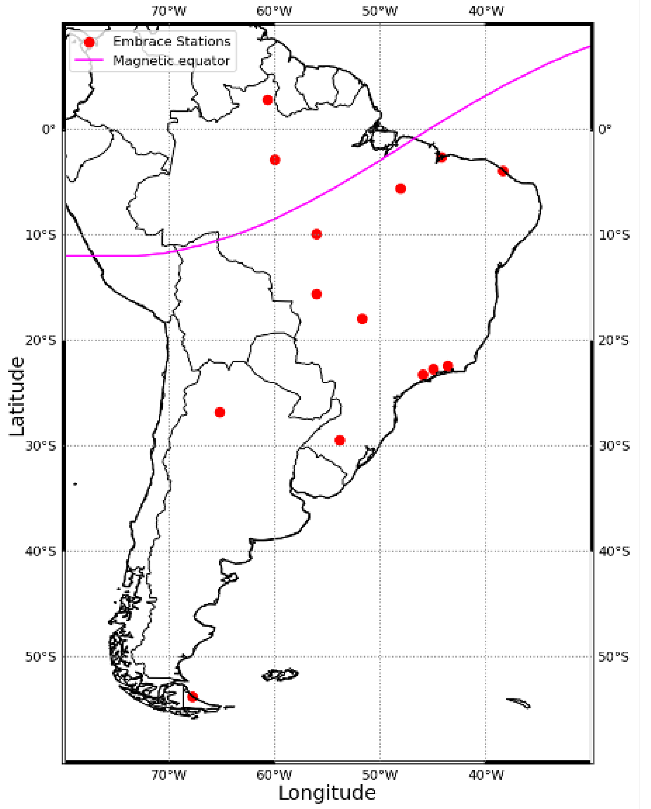
3.1. Database

The geomagnetic data utilized in this study are from the Embrace (Brazilian Study and Monitoring of Space Weather) magnetometer network, managed by the National Institute for Space Research (INPE). They began to be installed in 2010, and by 2014, the network comprised ten fluxgate magnetometers strategically located: nine across various regions of Brazil and one in southern Argentina. The latitudinal coverage ranges from 02 35 39 S to 53 47 09 S and the longitude from 38 25 28 W to 67 45 42 W , as shown in Figure 1. This deployment spans a significant latitudinal range, from low to high latitudes, encompassing key areas influenced by the Equatorial Electrojet and the SAMA.
The Earth’s magnetic field is a vector field described by its total intensity F and its components along three reference planes: the meridional (north–south), zonal (east–west), and vertical (nadir). The horizontal component H and the vertical component Z are projections of F at a given location, with Z considered negative when pointing upward, as in regions south of the magnetic equator. The components X and Y correspond to the north–south and east–west directions, respectively. The declination D is the angle between the geographic and magnetic north, while the inclination I is the angle between F and the horizontal plane. These components are related through trigonometric and vector relationships, and F is typically measured in nanoteslas (nT), where 1 T = 10 9 nT [8].
Magnetic field measurements can be scalar (measuring only F) or vectorial (measuring components such as X , Y , Z or H , D , Z ). Vector magnetometers are used for low-field (<1 mT) measurements and include types such as fluxgate, SQUID, Hall effect, and proton-precession magnetometers. Depending on the instrumentation and purpose, the data can be classified as absolute (instantaneous, using reference magnetometers) or relative (recording variations from a baseline using variometers). Complete geomagnetic field information requires at least three components, from which the rest can be derived.
The Embrace MagNet network utilizes three-axis fluxgate magnetometers to monitor geomagnetic variations with high precision. These sensors operate by inducing a magnetic field through an excitation coil that periodically saturates a soft ferromagnetic core and measuring the voltage induced in the sensing coils aligned with the core [17]. This configuration allows for the detection of both direct current (DC) and low-frequency alternating current (AC) magnetic fields, with sensitivity ranging up to 1 mT and resolution as fine as 10 pT . In practice, the system provides measurements with an amplitude resolution of 0.1 nT and sampling intervals as short as one second, enabling the acquisition of high-resolution geomagnetic data [18].
This work uses the 1 Hz resolution data of the H , D , and Z components. The measurements are stored in an ASCII file for each hour of the day. The hourly files were compiled into a single text file that contains data for the entire day. Not all files were complete, with the expected 86,400 data points. The missing data files were processed by inserting null values, that is, computationally defined as NaN (Not a Number), in the timestamp where data were missing. Data were collected from seven stations: São Luiz (SLZ), with 357 days available for analysis; Eusébio (EUS), Jataí (JAT), and Cachoeira Paulista (CXP), each with 361 days; São José dos Campos (SJC), with 350 days; São Martinho da Serra (SMS), with 356 days; Cuiaba (CBA) with 134 days; and Alta Floresta (ALF) with 123 days. Throughout 2014, the data presented the most continuous extension and best performance (no gaps) at most of the stations.
We compared geomagnetic pulsations during periods of high and low geomagnetic activity, classified using geomagnetic indices that quantify the intensity and characteristics of geomagnetic disturbances. Among the most commonly used indices are the (minute resolution) Auroral Electrojet (AE) index, which reflects activity in high-latitude auroral zones [19]; the (hourly) Disturbance Storm Time (Dst) index, which measures the ring current at mid and low latitudes [20]; and the planetary index K p , which provides a global measure of geomagnetic activity [21].
The K p index is a quasi-logarithmic scale ranging from 0 (quiet) to 9 (extremely disturbed), derived from 3 h measurements of geomagnetic variations recorded at mid-latitude observatories worldwide. It reflects planetary-scale geomagnetic disturbances, making it suitable for identifying quiet and active periods on a global basis [22]. To characterize geomagnetic activity in our study, we selected the five quietest and five most disturbed days of each month based on the K p index. The list of geomagnetically active and quiet days was obtained from the World Data Center for Geomagnetism, Kyoto (https://wdc.kugi.kyoto-u.ac.jp/wdc/Sec3.html, accessed on 1 March 2025), which releases data that select quiet and disturbed days using the algorithm developed at the GFZ in Potsdam, Germany (https://www.gfz.de/en/section/geomagnetism/data-products-services/kp-index/q/d-days-1 accessed on 1 March 2025). The selected days were then analyzed using wavelet-based techniques, specifically the continuous wavelet transform (CWT) and discrete wavelet transform (DWT). Both of them can treat non-stationary and non-linear phenomena data. These methods are well suited for identifying the frequency bands corresponding to different types of geomagnetic pulsations (Pc2 to Pc5) and for evaluating their intensity and spatial distribution across the network.
An innovation of this research is the development and implementation of a geomagnetic pulsation occurrence map and intensity quantification for South America. This is the first work to use high-resolution geomagnetic data from the MagNet network, utilizing the comprehensive dataset from 2014. The study provides unprecedented insights into the temporal and spatial patterns of geomagnetic pulsations, enhancing understanding of their impact across different geomagnetic and geographic contexts.

3.2. Methodology for the Signal Analysis

To dissect the complex time series data obtained from the Embrace magnetometer network, wavelet transform (WT) techniques were employed. These techniques are instrumental in breaking down non-stationary signals into time–frequency components, allowing a detailed analysis of the temporal and spectral characteristics of geomagnetic pulsations.
The WT is a linear transformation that is covariant under translation and dilation, making it well suited for analyzing signals with both localized and scale-dependent features. While the Fourier transform decomposes a signal into sine and cosine functions that are localized only in frequency, the wavelet transform uses basis functions that are localized in both time and frequency. This dual localization enables a balance between time and frequency resolution, constrained by the Heisenberg uncertainty principle, where the product of temporal and spectral resolutions is inversely proportional [23,24].
These properties make the wavelet transform particularly powerful for analyzing non-stationary signals, where statistical properties such as mean and variance vary over time. Wavelet analysis can detect localized structures and transient features in the signal, offering insights that traditional spectral techniques may overlook. For a function ψ ( t ) belonging to the space of square-integrable functions L 2 ( R ) , the wavelet function must satisfy two key conditions: (i) the admissibility condition, ensuring that the wavelet has zero mean and thus allows for perfect reconstruction of the original signal, and (ii) the unit energy, which implies that the function is either compactly supported or decays rapidly [23,24]. The wavelet transform coefficients reflect local properties of the signal: smooth regions yield small coefficients, while abrupt variations or singularities produce large responses. The term “wavelet function” is often used to refer to both orthogonal and non-orthogonal families. The continuous wavelet transform of a signal f ( t ) is defined as the following integral:
W ( a , b ) = f ( t ) ψ a , b ( t ) d t ,
where ψ a , b ( t ) = 1 a ψ t b a represents the scaled and translated version of the mother wavelet, with a and b denoting the scale and translation parameters, respectively [24].
The continuous wavelet transform (CWT) refers to Equation (1), where the scale and location parameters take continuous values. Visualization of these parameters in CWT is typically performed using wavelet spectra or scalograms, which represent the energy distribution of the signal over time by its scale [24,25]. The calculation of the wavelet coefficients W ( b , a ) can be performed numerically. However, the computational time is very high. This can be reduced if the coefficients are computed in the Fourier domain, rewriting the CWT in a way that allows for convolution theorem exploitation, as follows:
W ( b , a ) = a e i b ω ψ ^ * ( a ω ) f ^ ( ω ) d ω ,
where f ^ ( ω ) is the Fourier transform of f ( t ) [26,27].
CWT uses several families of wavelets. One of the most widely used is the complex Morlet wavelet, which consists of a plane wave modulated by a Gaussian function. Another commonly used wavelet is the Mexican Hat, which is the second derivative of the Gaussian function [28]. Other types of wavelets and their complete descriptions can be found in [29].
The choice of the wavelet function depends on the objective of the study and should reflect the characteristics of the time series. For example, for data with abrupt variations or steps, the Haar wavelet is recommended. Meanwhile, for smoother variations, the Morlet or Mexican Hat wavelets are preferred [24]. The complex Morlet wavelet is particularly suitable for capturing variations in the periodicities of geophysical signals [30], such as those in this study. It allows for analysis of amplitude and phase changes in the signal with good localization in both time and frequency.
The Morlet wavelet family consists of a plane wave modulated by a Gaussian function, expressed as follows:
ψ ( t ) = π 1 / 4 e i ω 0 t e ω 0 2 / 2 e t 2 / 2 ,
where ω 0 t is a dimensionless value. The Morlet wavelet will only have zero mean if a small correction term is added to Equation (3). Generally, ω 0 = 6 is adopted because it provides a good balance between time and frequency localization (in the context of the uncertainty principle). Furthermore, the correction terms become unnecessary, as they are of the same order as typical computer rounding errors [31,32].
Each scale a can be associated with a frequency f, where a low scale value corresponds to a high-frequency analysis. Similarly, a high scale value provides low-frequency information. However, despite this qualitative correspondence, there is no precise relationship between scale and frequency. Thus, it is more appropriate to establish a pseudo-frequency ω a corresponding to a given scale a, expressed as follows:
ω a = ω ψ a Δ t ,
where ω ψ is the central frequency associated with the wavelet and Δ t is the time interval between each signal sample [23,33].
Figure 2 illustrates an example of a scalogram generated from a synthetic signal containing wave packets at the frequencies of geomagnetic pulsations. The signal starts at t = 0 without oscillation. The first wave packet represents Pc1 pulsations, with a central frequency of 0.25 s , followed by additional packets representing Pc2, Pc3, Pc4, and Pc5 pulsations. After the separate wave packets, a white noise signal was added for a period, followed by the sum of all wave packets plus noise and then only the sum of the wave packets. In the next step, each packet was gradually subtracted.
This example highlights the ability of the CWT to identify present frequencies, locate them temporally, and detect background noise in the signal.
The Fourier transform (green line on the left panel) and the global wavelet spectrum highlight peaks corresponding to the wave packets in the signal, at 0.25 Hz , 0.125 Hz , 3.125 × 10 2 Hz , 1.56 × 10 2 Hz , and 1.95 × 10 3 Hz . Looking at the scalogram, we see higher wavelet coefficient intensities at scales corresponding to these pseudo-frequencies. However, the exact moments when the signal frequency changes are clearly visible in the scalogram.
Due to the redundancy of the CWT, its significance lies in its utility as a preliminary analysis tool for signal content, allowing for a comprehensive characterization of the information contained in the signal. However, the computational cost is high, with the number of operations on the order of N 2 , where N is the number of points in the time series.
In the discrete wavelet transform (DWT), the scale and translation parameters take discrete values. It can be redundant or not, depending on the function used and whether it is orthogonal. A signal f ( t ) is represented by a series of the following form:
f ( t ) = j = k = d j k ψ j k ( t )
where ψ j k ( t ) = ψ ( 2 j t k ) is the wavelet function or mother wavelet [23].
The wavelet coefficients d j k are given by the following:
d j k = 2 j f ( t ) ψ ( 2 j t k ) d t .
The coefficients d j k are also called details. They show the difference between two consecutive levels of signal decomposition.
The discrete orthogonal transform is built using a multi-resolution analysis (MR) tool. An MR is formed by the pair ( V j , ψ j ) , where V j is a closed subspace of L 2 ( R ) , formed by the functions φ k l that constitute a Riesz basis for this space [34].
In this technique, the mother wavelet function is generated by a scaling function that satisfies the following relation:
φ ( x ) = 2 k h ( k ) φ ( 2 x k ) ,
where φ ( x ) is called the scaling function and h ( k ) is a low-pass filter. Thus, the mother wavelet function is constructed as follows:
ψ ( x ) = k g ( k ) φ ( 2 x k ) ,
where g ( k ) = ( 1 ) k h ( 1 k ) is a high-pass filter.
The orthogonal wavelets of Daubechies are examples of this type of construction. More details can be found in [23].
There are several ways to implement a DWT algorithm. The most well-known is the Mallat algorithm (Mallat, 1989), also called the pyramidal algorithm. In this method, two filters, one smooth and one coarse, are built from the wavelet coefficients and used to obtain data for each scale.
DWT can be used to decompose a signal into successive levels of detail and approximation, such that a signal is divided into various resolution levels [35]. For example, a signal s can be decomposed into two orthonormal components: a low-frequency component (approximation a 1 ) and a high-frequency component (details d 1 ), such that s = a 1 + d 1 . The same process can be applied to the approximation a 1 , so that a 1 = a 2 + d 2 and s = a 2 + d 2 + d 1 , and so forth.
In this study, we use the orthogonal Meyer wavelet because it is a mother wavelet function with a frequency-limited band [36]. The scaling function in the Fourier domain of the Meyer wavelet is expressed as follows:
φ ^ ( ω ) = 1 2 π , | ω | < 2 π 3 , 1 2 π cos π 2 ξ 3 2 π | ω | 1 2 , 2 π 3 | ω | 4 π 3 , 0 , otherwise ,
where ξ ( ω ) , ω [ 0 , 1 ] is an interpolating polynomial with properties:
ξ ( ω ) = 0 , ω 0 , 1 , ω 1 .
The Meyer wavelet function is defined in the Fourier domain as follows:
ψ ^ ( ω ) = 1 2 π e i ω / 2 sin π 2 ξ 3 2 π | ω | 1 2 , 2 π 3 | ω | 4 π 3 , 1 2 π e i ω / 2 cos π 2 ξ 1 2 4 π 3 | ω | 1 2 , 4 π 3 | ω | 8 π 3 , 0 , otherwise .
Assuming a discrete time series with a sampling rate Δ t and number of points N (where N = 2 n , with n being an integer), the wavelet coefficients λ j , k are confined within 0 j n 1 and 0 k 2 j 1 . The frequency range for each j is given by 2 j / 3 T f 2 j + 2 / 3 T , where T is the length of the series ( T = N Δ t ) [36].
For a magnetogram with a resolution of 1 s, the number of points per day is N = 86,400. In the coefficient calculation process, zeros are added to the series until it reaches the next power of 2, extending the length of the series T = 131,072.
When analyzing signals, the constraints imposed by the instruments used must also be considered. In this case, the magnetometers’ sampling frequency defines the maximum detectable frequency, following the Sampling Theorem. If a continuous function f ( t ) sampled in the interval Δ is band-limited between f c and f c , then it is fully represented by its samples h n . The critical frequency, or Nyquist frequency, is expressed as follows [37]:
f c = 1 2 Δ .
If a signal is not band-limited within the Nyquist frequency, power spectrum components outside this range are falsely aliased into the range. This phenomenon is known as aliasing.
Considering the sampling rate, it is not possible to study pulsations with frequencies above the Nyquist frequency. The data used in this study have Δ t = 1 s , meaning that the critical frequency is f c = 1 / 2 Hz. Therefore, detectable pulsations are those with periods above 2 s , corresponding to Pc2 or higher.
This separation allows for the analysis of signals in the appropriate frequency bands, as shown in Table 1.
The continuous wavelet transform (CWT) was utilized primarily to analyze variations in the geomagnetic pulsation frequency over time. The CWT offers a scalable and localized spectral analysis, providing a means to identify the dominant modes of oscillations and their variations within the geomagnetic signals. This transform is particularly effective in detecting transient features and non-periodic components in geomagnetic data, such as sudden commencements or irregular pulsations. In conjunction with CWT, the discrete wavelet transform (DWT) was applied to segment the data into approximate and detail coefficients at various levels of decomposition. This approach is valuable for isolating specific frequency bands associated with different types of geomagnetic pulsations (e.g., Pc2 to Pc5). DWT’s MR analysis capability enables the extraction of significant trends and patterns from the geomagnetic data, which are essential for understanding the underlying geomagnetic processes.
The routines for the DWT calculations were developed in Python 3.11.0 based on the Wavelab package (https://statweb.stanford.edu/~wavelab/ accessed on 1 August 2023) [38]. This package provides various libraries with implementations of continuous and discrete wavelet transforms. Our Python complement contains only the DWT using Meyer wavelets for now and can be found at https://github.com/zemarchezi/pyWavelab, accessed on 1 March 2025. For the computation of the CWT, the routines of Torrence and Compo [27] were used, as they were suitable for this application. These routines were modified for the study of magnetogram data, as they were originally developed to analyze time series variations related to El Niño phenomena [27].
The wavelet analysis began with preprocessing steps that included detrending and normalization of the magnetometer data to remove non-geomagnetic noise and ensure uniformity in the dataset. Following this, wavelet filters were applied to the preprocessed data to extract relevant features for further analysis. The choice of wavelet base and scales was guided by the need to optimize the resolution in both the time and frequency domains, ensuring that the wavelet transforms could effectively capture the dynamics of geomagnetic pulsations across different scales. By applying both CWT and DWT, the study not only identifies the prevalent pulsation frequencies but also elucidates their distribution and changes over time and space. This dual approach ensures comprehensive coverage of the data’s spectral properties, facilitating a robust analysis of the geomagnetic environment’s dynamics.
The transform was applied to all days at each station using data with a resolution of one second. To minimize edge effects, a three-day consecutive period was used in the transform calculation, selecting only the coefficients corresponding to the second day while discarding the others. The scalograms for the first and last days of each month include a curve indicating the cone of influence. The selected scales for analysis range from 2 δ t , with δ t = 1 s , up to 2048. Since a Morlet wavelet with ω 0 = 6 was assumed—maximizing the balance between scale and frequency [27]—the variations highlighted by the CWT range from periods of 2 s to 2048 s .

4. Results and Discussion

Here, diagnostics regarding the presence of geomagnetic pulsations are presented in the records obtained by the Embrace MagNet. For the first time, in a permanent network, with a growing number of magnetometers, under the condition of calibrated and intercalibrated equipment in Brazil, it was possible to access a large-scale diagnosis that is easily perceptible to any interested user. Initially, illustrated by an example case, the basic result obtained through the application of wavelet transform methodology for signal analysis is presented. With the extension of this application to all available stations during the selected period of 2014, a broader analysis is conducted. Then, an analysis is performed by tabulating the occurrences on the basis of signal intensity. Finally, within the time constraints of this study, the first analysis was performed presenting the behavior by latitude in South America.

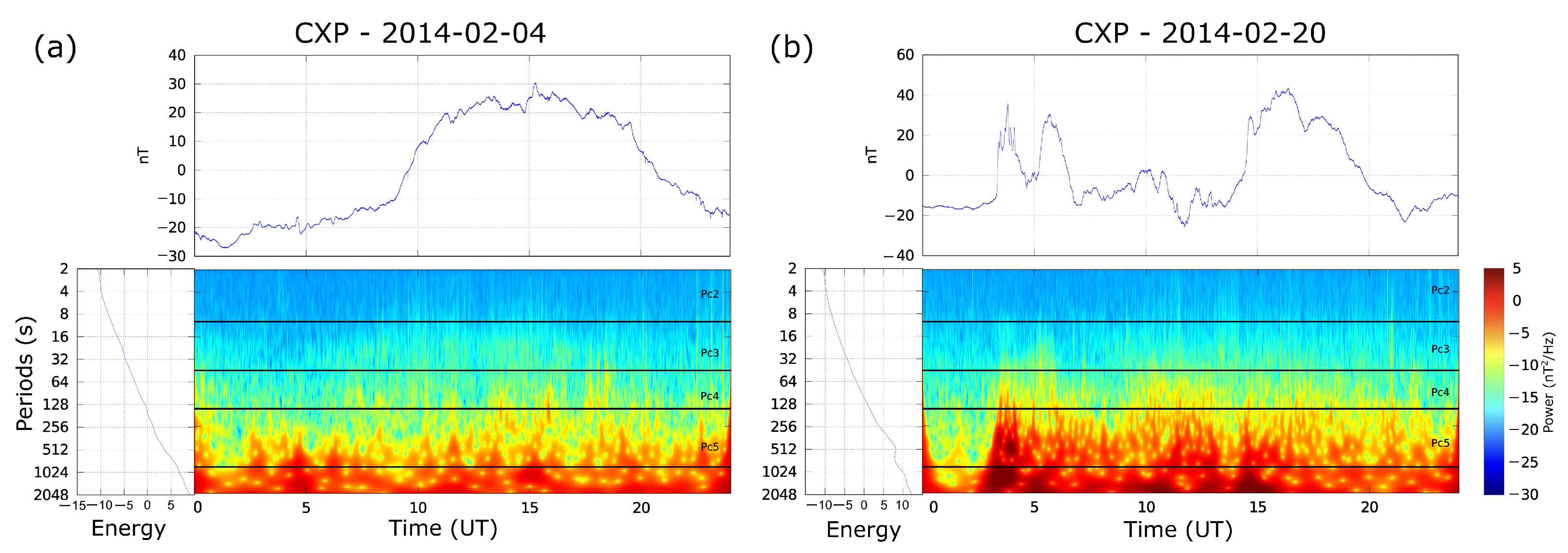
4.1. Diagnostic Analysis

Initially, analyses are conducted by applying the continuous wavelet transform (CWT) to the H, D, and Z components of the geomagnetic field for both quiet and disturbed days at each station separately. This approach allows for a comprehensive examination of the full spectrum of diurnal field variations and the identification of signal structures that may be linked to geomagnetic pulsations. The discrete wavelet transform (DWT) is then employed to extract information within more constrained frequency bands, providing a clearer characterization of signal intensities in specific frequency ranges. This step is essential because a broad-spectrum analysis alone often fails to capture the nuanced behaviors of geomagnetic pulsations.
As an illustrative case, Figure 3 shows the scalograms of the diurnal variation of the H component for a quiet day (a) and a disturbed day (b). The black horizontal lines in all scalograms delineate the frequency bands corresponding, from top to bottom, to Pc2, Pc3, Pc4, and Pc5. The upper panel shows the magnetic H component, where the vertical axis represents the intensity in nanoteslas, plotted against time on the horizontal axis. The lower panel displays the scalogram, where the color scale represents the signal intensity. The vertical axis indicates the frequency bands (pseudo-frequencies), plotted against time on the horizontal axis. The left panel shows the integrated spectrum of the signal. This type of graphical representation allows for a dynamic interpretation of the signal, which describes a physical process that is generally non-stationary and exhibits non-linear characteristics. From Figure 3, we can see that the intensity of the wavelet coefficient is higher on the disturbed day. Furthermore, some high-frequency fluctuations can be observed, reaching the Pc2 range around local noon ( 15 UT ) and during the evening hours.
Through a similar analysis, based on Figure S1 (Supporting Information), for the Rio Grande station in Argentina, external noise is also present in the signal. The diurnal variation contains a signal with a constant frequency close to 0.1 Hz , which falls within the Pc2–3 classification. However, this signal does not exhibit the impulsive characteristics or wave packet structures typical of continuous pulsations. This diagnosis suggests that the Rio Grande station needs to be further examined to determine the cause of this contamination in its measurements. All cases similar to this situation were excluded. The analysis was extended to all the stations used in this work for quiet and disturbed days. We used the H component of the geomagnetic field, since it is the one that presents the highest variations, and it is sufficient to identify the phenomena in this work.
Following the analysis for all stations and data, we observe that the characteristic diurnal variation of a geomagnetically quiet day is observed, with a smooth increase in the intensity of the H component around local noon. The scalograms present an increase in the intensity of the wavelet coefficients at local noon. Structures within the Pc5 range are more evident in all cases; however, shorter-period variations are also observed almost throughout the day, with an increase in intensities at noon.

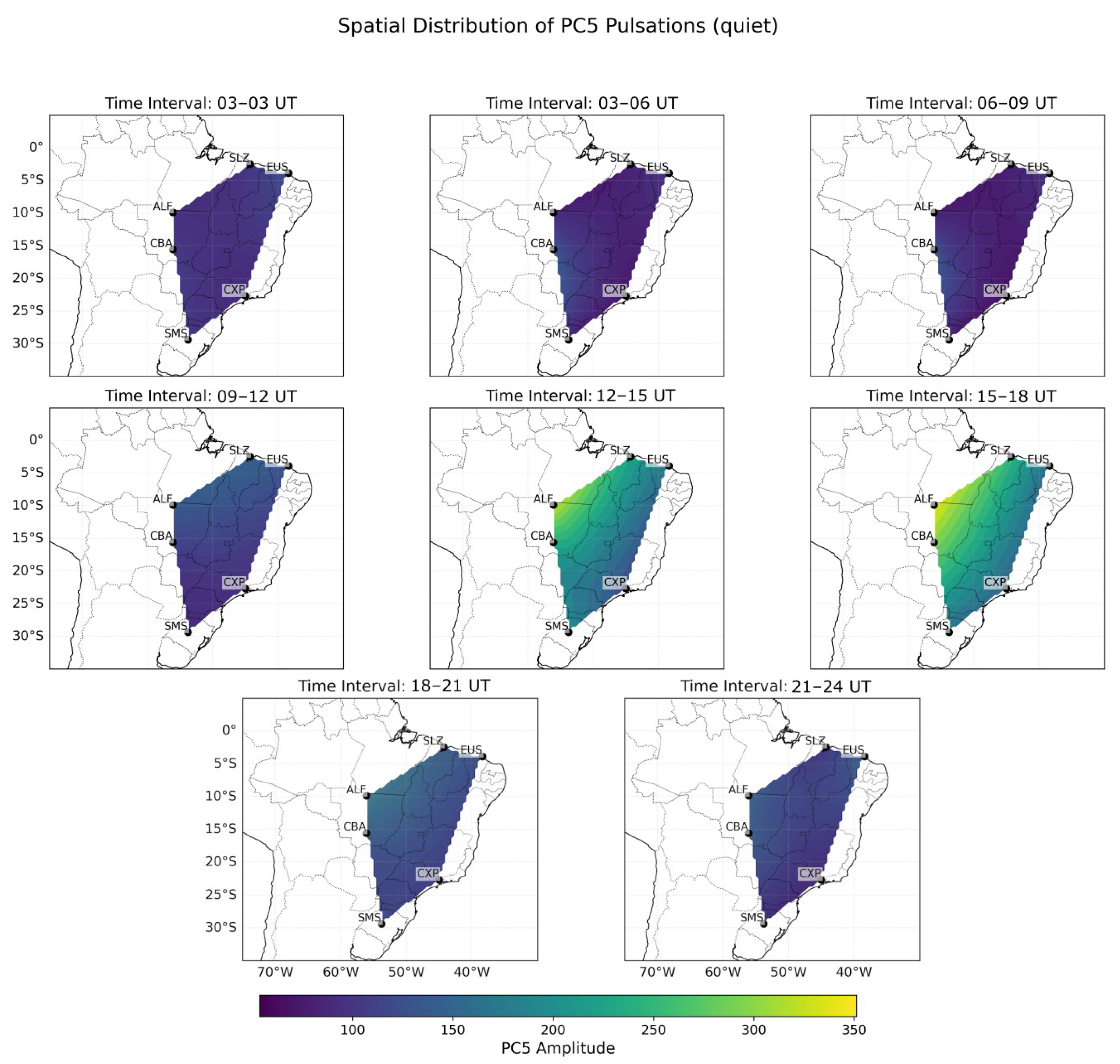
4.2. Latitudinal Behavior

The analysis of signals using the DWT allows for the examination of pulsations on the basis of the intensities of the reconstructed signals for each frequency band. An example of the signals corresponding to the analyzed frequency bands, reconstructed from the coefficients, is illustrated in Figure 4. The left side of the figure refers to measurements during a quiet period, while the right side corresponds to a disturbed period. The figure shows the variation of the signal in the pseudo-frequency band over time. Each panel represents a type of pulsation, respectively, from top to bottom: Pc5, Pc4, Pc3, and Pc2. The last panel displays the analyzed signal, which is the horizontal component of the geomagnetic field for the respective station. As a way to account for the occurrence or absence of pulsations in a given period, a minimum threshold was defined for the average intensities of the wavelet coefficients for both quiet and disturbed days. Above this threshold, it is assumed that significant magnetic activity has occurred.
The minimum value chosen for each frequency band at each station was the average intensity of the coefficients. For example, for the frequency range of Pc2, in CXP, the minimum value was 0.23 and the maximum value was 4.99 . The cutoff value was the mean value, which is 2.38 .
Figure 5 presents the hourly distribution of threshold-crossing events for continuous geomagnetic pulsations (Pc2–Pc5) at all Embrace geomagnetic stations during quiet and disturbed geomagnetic conditions. The percentage of time within each hour that the pulsation amplitude exceeded a predefined threshold is shown for each category of pulsations, with separate panels for quiet and disturbed periods. The red dashed lines in each panel indicate the overall average occurrence rate as a reference.
The results reveal distinct temporal patterns in the occurrence of threshold-crossing events. Under quiet geomagnetic conditions, the percentage of time in which the pulsation amplitudes exceed their respective thresholds remains relatively low across all Pc categories, with only modest increases during specific hours. Most threshold crossings occur during the midday and afternoon UT hours, but their frequencies are lower than those observed during disturbed conditions. This suggests that, in the absence of strong geomagnetic disturbances, the background pulsation activity remains relatively weak, with sporadic enhancements likely associated with regular solar-wind-driven magnetospheric dynamics.
In contrast, during disturbed periods, the frequency of threshold-crossing events increases considerably, particularly between 10 and 18 UT. This enhancement is most prominent in the higher-frequency pulsations (Pc4 and Pc5), where the exceedance rates reach 100 % in some hours, indicating that strong pulsations are nearly continuous during these times. The increased occurrence of intense pulsations during disturbed periods suggests that geomagnetic activity plays a crucial role in modulating the amplitude of these waves. The higher occurrence rates during the midday-to-afternoon UT hours are consistent with previous studies linking geomagnetic pulsation activity to ionospheric conductivity variations and solar-wind–magnetosphere interactions that intensify wave activity.
The observed differences between quiet and disturbed periods highlight the strong dependence of the pulsation intensity on geomagnetic activity. The threshold exceedance rates suggest that stronger pulsations occur preferentially when the magnetosphere is disturbed, likely because of enhanced wave–particle interactions and increased energy input from solar-wind fluctuations. These findings reinforce the idea that continuous geomagnetic pulsations are a key indicator of magnetospheric dynamics, with their intensity and frequency being strongly modulated by external driving forces such as solar wind pressure variations, interplanetary magnetic field conditions, and substorm activity.
Moreover, the results provide insight into the potential impact of these pulsations on space weather applications. Since strong pulsations have been linked to geomagnetically induced currents (GICs) and other space weather effects, the increased frequency of threshold exceedances during disturbed periods suggests that these events may have significant implications for technological systems, such as power grids and satellite operations [39]. The distinct diurnal variation observed, with peak activity occurring between 10 and 18 UT, suggests that pulsation activity follows a predictable pattern that could be incorporated into forecasting models for space weather mitigation strategies.
Figure 6 presents the hourly distribution of the average amplitude of the geomagnetic pulsations recorded at all Embrace geomagnetic stations during disturbed and quiet periods. The panels display the temporal evolution of different pulsation categories, providing insight into how their intensity varies under different geomagnetic conditions.
Panels (a) and (b) illustrate the hourly variation of Pc2 amplitudes during disturbed and quiet periods, respectively. The amplitude exhibits a pronounced increase around 12 to 15 UT in both cases; however, during disturbed periods, the pulsation intensity is significantly enhanced. The mean and median values, as well as the standard deviation, indicate greater variability under disturbed conditions, suggesting that geomagnetic disturbances amplify Pc2 activity, leading to more pronounced fluctuations. A similar pattern is observed in panels (c) and (d), which display the behavior of Pc3 pulsations. During disturbed periods, the amplitude is substantially higher, with a peak occurring between 10 and 15 UT . Compared to the quiet period, Pc3 activity is more intense and exhibits greater variability, reinforcing the idea that geomagnetic disturbances strongly modulate the occurrence and intensity of these pulsations.
The amplitude of Pc4 pulsations, presented in panels (e) and (f), also shows a clear dependence on geomagnetic activity levels. During disturbed periods, Pc4 shows a significant increase, particularly between 10 and 18 UT , with a much wider range of variability, as indicated by the standard deviation. In contrast, quiet periods are characterized by a lower amplitude and a more gradual variation throughout the day. Panels (g) and (h) represent the distribution of Pc5 pulsations, which exhibit the most pronounced variations. During disturbed periods, the amplitude reaches values exceeding 600 nT, with a peak occurring between 12 and 18 UT . This dramatic increase in intensity suggests that Pc5 pulsations are particularly sensitive to geomagnetic disturbances. In contrast, during quiet periods, the amplitude remains significantly lower and the variability is significantly reduced.
Overall, the results indicate that continuous geomagnetic pulsations are strongly modulated by geomagnetic activity, with amplitudes consistently higher during disturbed periods, especially from midday to the afternoon in UT time. The shaded regions in the plots, representing the standard deviation, further emphasize the greater dispersion of the data during geomagnetically disturbed conditions. Comparison with the occurrence of pulsations during geomagnetically disturbed days shows a significant increase in activity. In particular, Pc4 and Pc5 pulsations become more prominent, indicating a stronger contribution from magnetospheric instabilities, reconnection processes, and substorm activity. The enhancement of Pc2 and Pc3 pulsations under disturbed conditions suggests an intensification of the solar-wind–magnetosphere interactions, leading to increased energy transfer into the Earth’s magnetic field. This response is especially notable at lower latitudes, where ionospheric coupling mechanisms influence the occurrence of geomagnetic pulsations.
The results provide important insights into the underlying physical processes that govern geomagnetic pulsations. The observed differences between quiet and disturbed days reinforce the idea that geomagnetic activity plays a fundamental role in shaping the pulsation characteristics. Furthermore, the temporal variation of the pulsation intensity suggests a strong dependence on magnetospheric conditions, highlighting the importance of external drivers such as solar wind pressure, interplanetary magnetic field orientation, and ionospheric conductivity. Statistical analysis of Pc2 to Pc5 pulsations reveals a clear dependence on geomagnetic conditions, local time, and station location. The local time dependence on geomagnetic pulsations agrees with previous studies. Ref. [40] investigated Pc3-4 geomagnetic pulsations at very low and equatorial latitudes and presented a dependence of local time with a greater occurrence of those fluctuations around midday. Ref. [41] analyzed geomagnetic pulsations in five observatories and confirmed that pulsation activity clusters by local time, especially near magnetic noon, supporting the influence of solar-driven ionospheric changes. Ref. [11] observed these variations with the day–night asymmetry of magnetospheric current systems and solar wind input, highlighting a stronger pulsation power on the dayside due to higher solar wind pressure and conductivity.
Understanding these patterns is crucial for advancing space weather forecasting and improving models of geomagnetic disturbances. The findings presented here contribute to a broader understanding of how the Earth’s magnetic field responds to variations in solar wind activity, offering insight into the complex interplay between the magnetosphere and the ionosphere. Further studies incorporating extended datasets and higher-resolution observations could provide a more detailed characterization of pulsation behavior under different space weather conditions.
With the data filtered at the respective frequencies, the analysis of the signal amplitude was carried out according to the geographical location of the station. Data for quiet and disturbed days were separated for each station. The average of the modulus of the wavelet coefficient intensities corresponding to each pulsation class was computed for the quiet and disturbed days of each month. Using these values, graphs were generated showing the intensities of each class according to time, separated into (00–03), (03–06), (06–09), (09–12), (12–15), (15–18), (18–21), (21–24) universal time sectors.
To illustrate, Figure 7 and Figure 8 show the average intensity of the Pc5 geomagnetic pulsations over the stations during quiet periods and disturbed periods. The intensity of occurrence is indicated by a color bar.
Figure 7 illustrates the spatial distribution of the pulsation amplitudes of the geomagnetic pulsation of Pc5 across the network of the Embrace geomagnetic station under quiet geomagnetic conditions. The maps are organized into eight panels, each representing a three-hour interval, providing information on the diurnal variation of pulsation intensity. The color scale in each panel denotes the amplitude of Pc5 pulsations, with darker colors corresponding to lower intensities and brighter colors indicating stronger pulsations.
The results reveal a pronounced diurnal variation in Pc5 pulsation activity. During the early morning hours (00–09 UT), the pulsation amplitudes remain relatively low and uniformly distributed throughout the monitored region. As the day progresses, a significant increase in pulsation intensity is observed, particularly between 12 and 18 UT, with the highest amplitudes concentrated in the northern and central regions of the observation area. After this peak period, pulsation activity gradually declines towards the evening and night hours (18–24 UT), returning to lower amplitude levels similar to those observed in the early morning.
This diurnal trend aligns with previous studies that have linked the occurrence of Pc5 pulsations to solar wind and Earth’s magnetosphere interactions, which are modulated by changes in ionospheric conductivity throughout the day. The enhancement of Pc5 amplitudes around local noon and early afternoon (12–18 UT) suggests a possible influence of increased ionospheric conductivity due to solar radiation. Furthermore, the observed spatial variation in the intensity of the pulsation can be attributed to the differences in ionospheric conductivity and geomagnetic latitude, which can influence the efficiency of wave penetration from the magnetosphere into the ionosphere and onto the ground [42].
Figure 8 illustrates the spatial distribution of Pc5 geomagnetic pulsation amplitudes across the Embrace geomagnetic station network during disturbed geomagnetic conditions. The eight panels represent different three-hour universal time (UT) intervals, allowing for a detailed examination of the diurnal variation of the pulsation intensity. The color scale in each panel indicates the pulsation amplitude, with darker colors corresponding to lower intensities and brighter colors representing stronger pulsations.
Compared to quiet conditions, the results reveal a substantial increase in Pc5 pulsation amplitudes during disturbed periods. Although the pulsation intensity remains relatively low during the early morning hours (00–09 UT), there is a clear enhancement that begins around 09 UT , with the highest amplitudes occurring between 12 and 18 UT . During this period, pulsation activity becomes significantly more intense, with amplitudes reaching values more than twice as high as those observed under quiet conditions. The increased intensity persists until approximately 21 UT, after which the pulsation amplitudes gradually decrease towards pre-disturbance levels.
The pronounced enhancement of Pc5 amplitudes during disturbed conditions suggests a strong link between geomagnetic activity and pulsation generation mechanisms. Pc5 pulsations are known to be associated with ULF wave activity in the magnetosphere, often driven by variations in solar wind pressure, substorm activity, and wave–particle interactions. The observed increase in amplitude during disturbed periods is consistent with previous studies indicating that enhanced solar-wind–magnetosphere coupling leads to stronger pulsation excitation.
Furthermore, the spatial distribution of the intensity of the pulsation exhibits regional variability, with the highest amplitudes occurring in the northern and central portions of the monitored area. This may be attributed to differences in local ground conductivity, ionospheric coupling effects, and magnetospheric resonance conditions that influence wave propagation and amplification. The broader spatial extent of high-amplitude pulsations during disturbed conditions further supports the idea that geomagnetic storms and substorms contribute to the large-scale excitation of ULF waves in the magnetosphere. Although the main discussion in the spatial distribution focuses on Pc5 pulsations due to their broader spatial signatures and clearer diurnal modulation, analyses for Pc2, Pc3, and Pc4 pulsations were also performed following the same methodology. The results, including corresponding amplitude maps and diurnal variation plots under both quiet and disturbed conditions, are provided in the Supporting Information for reference and comparison.
The diurnal variation observed in the disturbed period highlights the role of ionospheric conductivity changes in modulating pulsation activity. The peak intensities around midday and early afternoon UT may be linked to enhanced ionospheric conductivity due to solar radiation, which facilitates the penetration of magnetospheric waves into the ionosphere and onto the ground. Furthermore, the increased occurrence of strong Pc5 pulsations during disturbed conditions has important implications for space weather studies, as these waves have been associated with the acceleration and transport of energetic particles in the magnetosphere, as well as the induction of geomagnetically induced currents (GICs) in power grids and pipelines [43,44].
Taking into account all the cases, a more descriptive characterization of the processes occurring in the magnetosphere–ionosphere system can be pursued. Field lines are known to transmit information from various regions in the form of waves that can be detected on the ground [45,46]. However, there are still local processes that need to be better understood. Through this study, based on the research conducted and the results obtained, it became evident that this is an emerging area of study, particularly considering the possibilities of remote sensing for various processes and even its potential application in Space Weather programs.

5. Conclusions

This study applied continuous wavelet transform (CWT) and discrete wavelet transform (DWT) techniques to analyze geomagnetic field variations recorded by the Embrace magnetometer network. By examining data from 2014, a year with optimal station coverage and minimal data gaps, we systematically investigated geomagnetic pulsations (Pc2–Pc5) under both quiet and disturbed geomagnetic conditions. The dataset covered a broad latitudinal range in South America, enabling a comprehensive spatial and temporal analysis of the characteristics of geomagnetic pulsation.
Specifically, as the continuous wavelet transform technique results show, the coefficient intensities indicate the prevalence of structures in the Pc5 range during disturbed geomagnetical days. However, the wavelet coefficients on quiet days indicate some structures occurring around local noon. Using the discrete wavelet transform technique for the PC-pulsation signal reconstructions, results highlight the visible difference in signal intensities when geomagnetic storms occur. Hourly distributions of threshold-crossing events for geomagnetic pulsations, mainly Pc2 to Pc5, help to identify distinct temporal patterns, indicating that strong pulsations are nearly continuous during geomagnetic storms. The hourly distributions of the average amplitudes of the geomagnetic pulsations recorded at all Embrace geomagnetic stations during disturbed and quiet periods exhibit a pronounced increase around 9 to 12 h (local time) in both cases; nevertheless, the pulsation intensities in disturbed periods are more intense and spread farther than the ones in quiet periods. The methodological approach developed allows us to obtain, concerning the local time, the spatial distributions (i.e., maps) of Pc5 geomagnetic pulsation amplitudes over the Embrace network during quiet and disturbed geomagnetic conditions. In the quiet regime, activity is located close to the dip equator line, and in the disturbed regime, intense activity spreads far away from the dip equator.
As a general result, the work confirms that geomagnetic pulsations are strongly modulated by geomagnetic activity. Under disturbed conditions, the pulsation amplitudes increase significantly, particularly for Pc4 and Pc5 pulsations, which exhibit a diurnal peak between 9 and 15 h ( local time ) . This finding in South America suggests an intensified energy transfer from the solar wind to the magnetosphere–ionosphere system, enhancing wave activity.
The use of wavelet transforms in this study represents a significant advancement in the analysis of geomagnetic pulsations. Unlike traditional spectral methods, wavelet analysis enables simultaneous resolution in both time and frequency domains, allowing us to capture transient pulsation events and their diurnal variations with high precision. This is particularly relevant for irregular and mixed pulsations whose signatures evolve rapidly. Moreover, the combination of CWT and DWT proved effective in identifying both global and localized wave activity, revealing spatial patterns that may be masked by more conventional techniques.
Strong Pc4 and Pc5 pulsations have been linked to geomagnetically induced currents (GICs), which can affect power grids, pipelines, and satellite systems. The distinct diurnal variation of pulsation activity suggests that pulsation occurrence follows a predictable pattern, which could be used for space weather forecasting and mitigation strategies. The results also reinforce the importance of low-latitude magnetometer networks in improving our understanding of global geomagnetic pulsation dynamics, particularly in regions affected by unique phenomena such as the SAMA and the Equatorial Electrojet.
Future work should focus on expanding the analysis to longer time series and multiple solar cycles, allowing for the assessment of long-term trends in pulsation behavior. Furthermore, incorporating data from other magnetometer networks and combining them with satellite observations would provide a more detailed characterization of ULF wave excitation mechanisms and their impact on the coupled magnetosphere–ionosphere system. Finally, further exploration of pulsation-related GIC effects in South America would be valuable in assessing regional vulnerabilities to space weather events.
This study provides a novel and detailed characterization of geomagnetic pulsations over South America, demonstrating their dependence on geomagnetic activity and their spatial and temporal variability. The findings contribute to a better understanding of magnetospheric dynamics and space weather interactions, with potential applications in space weather prediction, geomagnetic hazard assessment, and magnetosphere–ionosphere coupling studies.

Supplementary Materials

The following supporting information can be downloaded at: https://www.mdpi.com/article/10.3390/atmos16060742/s1, Figure S1: Scalogram of the H component of the magnetic field recorded at the Rio Grande station during the month of September 2014; Figure S2: Spatial distribution of Pc2 geomagnetic pulsation amplitudes over the Embrace network during quiet geomagnetic conditions; Figure S3: Spatial distribution of Pc2 geomagnetic pulsation amplitudes over the Embrace network during disturbed geomagnetic conditions; Figure S4: Spatial distribution of Pc3 geomagnetic pulsation amplitudes over the Embrace network during quiet geomagnetic conditions; Figure S5: Spatial distribution of Pc3 geomagnetic pulsation amplitudes over the Embrace network during disturbed geomagnetic conditions; Figure S6: Spatial distribution of Pc4 geomagnetic pulsation amplitudes over the Embrace network during quiet geomagnetic conditions; Figure S7: Spatial distribution of Pc4 geomagnetic pulsation amplitudes over the Embrace network during disturbed geomagnetic conditions.

Author Contributions

Conceptualization, J.P.M., O.M., and C.M.D.; methodology, J.P.M.; software, J.P.M.; validation, J.P.M., O.M., and C.M.D.; formal analysis, J.P.M. and O.M.; resources, J.P.M., O.M., and C.M.D.; data curation, J.P.M.; writing—original draft preparation, J.P.M.; writing—review and editing, O.M. and C.M.D.; visualization, J.P.M.; funding acquisition, O.M. and C.M.D. All authors have read and agreed to the published version of the manuscript.

Funding

This research was supported by the National Council for Scientific and Technological Development (CNPq) grants 134331/2014-1 and 302675/2021-3.

Institutional Review Board Statement

Not applicable.

Informed Consent Statement

Not applicable.

Data Availability Statement

All the data used in this work are publicly available at https://www2.inpe.br/climaespacial/portal accessed on 1 August 2023.

Acknowledgments

The authors would like to acknowledge the INPE Embrace program for providing all the data for Embrace/MagNet (http://www.inpe.br/spaceweather, accessed on 1 February 2025) used in this work, Margarete Oliveira Domingues, for all discussions on Wavelet methodology, and Varlei Everton Menconi for the proficous interaction about computational resources. JPM thanks CNPq/MCTI (Grant 134331/2014-1), and CMD thanks CNPq/MCTI (Grant 302675/2021-3). We thank the Brazilian Ministry of Science, Technology, and Innovations (MCTI) and the Brazilian Space Agency (AEB).

Conflicts of Interest

The authors declare no conflict of interest.

References

  1. Jacobs, J.A. Geomagnetism; Number v. 4 in Geomagnetism; Academic Press: London, UK, 1991; p. 806. [Google Scholar]
  2. Parker, E.N. Dynamics of the Interplanetary Gas and Magnetic Fields. Astrophys. J. 1958, 128, 664. [Google Scholar] [CrossRef]
  3. Kivelson, M.G.; Russell, C.T. Introduction to Space Physics; Cambridge University Press: Cambridge, UK, 1995. [Google Scholar] [CrossRef]
  4. Kivelson, M.G. Planetary magnetospheres. In Handbook of Solar-Terrestrial Environment; Springer: Berlin/Heidelberg, Germany, 2007; pp. 469–492. [Google Scholar] [CrossRef]
  5. Hargreaves, J.K. The Solar-Terrestrial Environment: An Introduction to Geospace–the Science of the Terrestrial Upper Atmosphere, Ionosphere, and Magnetosphere; Cambridge Atmospheric and Space Science Series; Cambridge University Press: Cambridge, UK, 1992. [Google Scholar]
  6. Schunk, R.W.; Nagy, A.F. Ionospheres, 2nd ed.; Cambrigde University Press: Cambridge, UK, 2009; Volume 82, p. 628. [Google Scholar]
  7. Lopez, R.E.; Gonzalez, W.D. Magnetospheric balance of solar wind dynamic pressure. Geophys. Res. Lett. 2017, 44, 2991–2999. [Google Scholar] [CrossRef]
  8. Merrill, R.T.; McFadden, P.L.; McElhinny, M.W. The Magnetic Field of the Earth, ilustrada ed.; International Geophysics Series; Academic Press: San Diego, CA, USA, 1998; p. 531. [Google Scholar]
  9. Saito, T. Geomagnetic pulsations. Space Sci. Rev. 1969, 10, 319–412. [Google Scholar] [CrossRef]
  10. Kelley, M.C. The Earth’s Ionosphere; International Geophysics; Elsevier Science: Amsterdam, The Netherlands, 2009. [Google Scholar]
  11. McPherron, R.L. Magnetic pulsations: Their sources and relation to solar wind and geomagnetic activity. Surv. Geophys. 2005, 26, 545–592. [Google Scholar] [CrossRef]
  12. Hughes, W.J. Magnetospheric ULF Waves: A Tutorial With a Historical Perspective. In Solar Wind Sources of Magnetospheric Ultra-Low-Frequency Waves; Engebretson, M.J., Takahashi, K., Scholer, M., Eds.; American Geophysical Union: Washington, DC, USA, 1994; pp. 1–11. [Google Scholar] [CrossRef]
  13. Jacobs, J.a.; Kato, Y.; Matsushita, S.; Troitskaya, V.a. Classification of geomagnetic micropulsations. J. Geophys. Res. 1964, 69, 180–181. [Google Scholar] [CrossRef]
  14. Baumjohann, W.; Treumann, R.A. Basic Space Plasma Physics; World Scientific: Singapore, 2012. [Google Scholar]
  15. Glaßmeier, K.H. Geomagnetic pulsations. In Encyclopedia of Geomagnetism and Paleomagnetism; Springer: Berlin/Heidelberg, Germany, 2007; pp. 333–334. [Google Scholar]
  16. Jacobs, J.A.; Jacobs, J. The Morphology of Geomagnetic Micropulsations; Springer: Berlin/Heidelberg, Germany, 1970. [Google Scholar]
  17. Ripka, P. Review of fluxgate sensors. Sens. Actuators A Phys. 1992, 33, 129–141. [Google Scholar] [CrossRef]
  18. Denardini, C.; Chen, S.; Resende, L.C.A.; Moro, J.; Bilibio, A.; Fagundes, P.R.; Gende, M.A.; Cabrera, M.A.; Bolzan, M.; Padilha, A.L.; et al. The embrace magnetometer network for South America: Network description and its qualification. Radio Sci. 2018, 53, 288–302. [Google Scholar] [CrossRef]
  19. Davis, T.N.; Sugiura, M. Auroral electrojet activity index AE and its universal time variations. J. Geophys. Res. 1966, 71, 785–801. [Google Scholar] [CrossRef]
  20. Sugiura, M. Hourly Values of Equatorial Dst for the IGY; Technical Report; NASA Goddard Space Flight Center: Greenbelt, MD, USA, 1963.
  21. Bartels, J. The geomagnetic measures for the time-variations of solar corpuscular radiation, described for use in correlation studies in other geophysical fields. Ann. Intern. Geophys. 1957, 4, 227–236. [Google Scholar]
  22. Matzka, J.; Stolle, C.; Yamazaki, Y.; Bronkalla, O.; Morschhauser, A. The geomagnetic Kp index and derived indices of geomagnetic activity. Space Weather 2021, 19, e2020SW002641. [Google Scholar] [CrossRef]
  23. Daubechies, I. Ten Lectures on Wavelets; CBMS-NSF Regional Conference Series in Applied Mathematics; SIAM: Philadelphia, PA, USA, 1992; Volume 61, p. 357. [Google Scholar] [CrossRef]
  24. Domingues, M.O.; Mendes, O.; da Costa, A.M. On wavelet techniques in atmospheric sciences. Adv. Space Res. 2005, 35, 831–842. [Google Scholar] [CrossRef]
  25. Castilho, J.E.; Domingues, M.O.; Pagamisse, A.; Mendes, O. Introdução ao Mundo das Wavelets, Notas em Matemática Aplicada; SBMAC: Sao Carlos, Brazil, 2012; Volume 62, 144p. [Google Scholar]
  26. Meyers, S.D.; Kelly, B.G.; O’Brien, J.J. An Introduction to Wavelet Analysis in Oceanography and Meteorology: With Application to the Dispersion of Yanai Waves. Mon. Weather Rev. 1993, 121, 2858–2866. [Google Scholar] [CrossRef]
  27. Torrence, C.; Compo, G.P. A Practical Guide to Wavelet Analysis. Bull. Am. Meteorol. Soc. 1998, 79, 61. [Google Scholar] [CrossRef]
  28. Lau, K.M.; Weng, H. Climate signal detection using wavelet transform: How to make a time series sing. Bull. Am. Meteorol. Soc. 1995, 76, 2391–2402. [Google Scholar] [CrossRef]
  29. Chui, C.K. An Introduction to Wavelets; Wavelet Analysis and Its Applications; Academic Press: San Diego, CA, USA, 1992. [Google Scholar]
  30. Weng, H.; Lau, K.M. Wavelets, Period Doubling, and Time-Frequency Localization with Application to Organization of Convection over the Tropical Western Pacific. J. Atmos. Sci. 1994, 51, 2523–2541. [Google Scholar] [CrossRef]
  31. Grinsted, A.; Moore, J.C.; Jevrejeva, S. Application of the cross wavelet transform and wavelet coherence to geophysical time series. Nonlinear Process. Geophys. 2004, 11, 561–566. [Google Scholar] [CrossRef]
  32. Farge, M. Wavelet Transforms and Their Applications To Turbulence. Annu. Rev. Fluid Mech. 1992, 24, 395–457. [Google Scholar] [CrossRef]
  33. Kumar, P.; Foufoula-Georgiou, E. Wavelet analysis for geophysical applications. Rev. Geophys. 1997, 35, 385. [Google Scholar] [CrossRef]
  34. Mendes, O.; Domingues, M.O.; Mendes da Costa, A.; Clúa de Gonzalez, A.L.; Oliveira Domingues, M.; Mendes da Costa, A.; Clúa de Gonzalez, A.L. Wavelet analysis applied to magnetograms: Singularity detections related to geomagnetic storms. J. Atmos. Sol. Terr. Phys. 2005, 67, 1827–1836. [Google Scholar] [CrossRef]
  35. Percival, D.B.; Walden, A.T. Wavelet Methods for Time Series Analysis; Cambridge Series in Statistical and Probabilistic Mathematics; Cambridge University Press: Cambridge, UK, 2006. [Google Scholar]
  36. Nosé, M.; Iyemori, T.; Takeda, M.; Kamei, T.; Milling, D.; Orr, D.; Singer, H.; Worthington, E.; Sumitomo, N. Automated detection of Pi 2 pulsations using wavelet analysis: 1. Method and an application for substorm monitoring. Earth Planets Space 1998, 50, 773–783. [Google Scholar] [CrossRef]
  37. Press, W.H. Numerical Recipes, 3rd ed.; Cambridge University Press: Cambridge, UK, 2007; 1235p. [Google Scholar] [CrossRef]
  38. Buckheit, J.B.; Donoho, D.L. Wavelab and Reproducible Research; Springer: Berlin/Heidelberg, Germany, 1995. [Google Scholar]
  39. Heyns, M.J.; Lotz, S.I.; Gaunt, C.T. Geomagnetic Pulsations Driving Geomagnetically Induced Currents. Space Weather 2021, 19, e2020SW002557. [Google Scholar] [CrossRef]
  40. Zanandrea, A.; Da Costa, J.; Dutra, S.; Trivedi, N.B.; Kitamura, T.; Yumoto, K.; Tachihara, H.; Shinohara, M.; Saotome, O. Pc3-4 geomagnetic pulsations at very low latitude in Brazil. Planet. Space Sci. 2004, 52, 1209–1215. [Google Scholar] [CrossRef]
  41. Orr, D.; Webb, D. Statistical studies of geomagnetic pulsations with periods between 10 and 70 sec and their relationship to the plasmapause region. Planet. Space Sci. 1975, 23, 1169–1178. [Google Scholar] [CrossRef]
  42. Espinosa, K.V.; Padilha, A.L.; Alves, L.R. Effects of ionospheric conductivity and ground conductance on geomagnetically induced currents during geomagnetic storms: Case studies at low-latitude and equatorial regions. Space Weather 2019, 17, 252–268. [Google Scholar] [CrossRef]
  43. Pulkkinen, A.; Bernabeu, E.; Thomson, A.; Viljanen, A.; Pirjola, R.; Boteler, D.; Eichner, J.; Cilliers, P.; Welling, D.; Savani, N.; et al. Geomagnetically induced currents: Science, engineering, and applications readiness. Space Weather 2017, 15, 828–856. [Google Scholar] [CrossRef]
  44. Engebretson, M.J.; Simms, L.E.; Pilipenko, V.A.; Bouayed, L.; Moldwin, M.B.; Weygand, J.M.; Hartinger, M.D.; Xu, Z.; Clauer, C.R.; Coyle, S.; et al. Geomagnetic disturbances that cause GICs: Investigating their interhemispheric conjugacy and control by IMF orientation. J. Geophys. Res. Space Phys. 2022, 127, e2022JA030580. [Google Scholar] [CrossRef]
  45. Le, G.; Liu, G.; Yizengaw, E.; Wu, C.C.; Zheng, Y.; Vines, S.; Buzulukova, N. Responses of field-aligned currents and equatorial electrojet to sudden decrease of solar wind dynamic pressure during the March 2023 geomagnetic storm. Geophys. Res. Lett. 2024, 51, e2024GL109427. [Google Scholar] [CrossRef]
  46. Oliveira, D. Ionosphere-magnetosphere coupling and field-aligned currents. Rev. Bras. Ensino Física 2014, 36, 1305. [Google Scholar] [CrossRef]
Figure 1. Distribution of Embrace MagNet magnetic station locations. The points in red are the stations. The magenta line represents the geomagnetic equator, which has a strongly tilted inclination compared to the geographical equator.
Atmosphere 16 00742 g001
Figure 2. Scalogram and global wavelet spectrum of a synthetic signal representing wave packets with the characteristic frequencies of geomagnetic pulsations. The top panel presents the time series, while the middle panel shows the scalogram, with the horizontal axis representing time and the vertical axis displaying signal periods. In the bottom left panel, the global wavelet spectrum is presented, obtained by integrating over time for each scale (shown in blue), alongside the Fourier transform of the signal (green). The horizontal axis represents the spectral intensity.
Atmosphere 16 00742 g002
Figure 3. Scalogram of the diurnal variation in the H component of the geomagnetic field, in the Cachoeira Paulista (CXP) station, during (a) a quiet day (4 February 2014) and (b) a disturbed day (20 February 2014).
Atmosphere 16 00742 g003
Figure 4. Variation of the H component of the geomagnetic field, in Cachoeira Paulista, on (a) 4 February 2014 and (b) 20 February 2014.
Atmosphere 16 00742 g004
Figure 5. Hourly distribution of threshold-crossing events for continuous geomagnetic pulsations (Pc2–Pc5) at all Embrace geomagnetic stations during quiet (left panels) and disturbed (right panels) periods. Each panel represents the percentage of time within each hour that the amplitude of a given pulsation type exceeded a predefined threshold, as indicated in the panel titles. The blue bars show the percentage of occurrences, while the red dashed lines indicate the overall average occurrence rate for reference. A clear diurnal pattern is observed, with a higher frequency of threshold crossings occurring during disturbed periods, particularly between 10 and 18 UT. This trend is more pronounced in higher-order pulsations (Pc4 and Pc5), where threshold exceedances are more frequent and persistent under disturbed conditions.
Atmosphere 16 00742 g005
Figure 6. Hourly distribution of the average amplitude of continuous geomagnetic pulsations (Pc2–Pc5) recorded across all Embrace geomagnetic stations during geomagnetically quiet (left panels) and disturbed (right panels) periods. The blue lines represent the average pulsation amplitude, while the red dashed lines indicate the median values. The shaded regions correspond to one standard deviation above and below the mean, illustrating the variability in pulsation intensity. (a) Pc2 amplitude during quiet periods; (b) Pc2 amplitude during disturbed periods; (c) Pc3 amplitude during quiet periods; (d) Pc3 amplitude during disturbed periods; (e) Pc4 amplitude during quiet periods; (f) Pc4 amplitude during disturbed periods; (g) Pc5 amplitude during quiet periods; (h) Pc5 amplitude during disturbed periods.
Atmosphere 16 00742 g006
Figure 7. Spatial distribution of Pc5 geomagnetic pulsation amplitudes over the Embrace network during quiet geomagnetic conditions. Each panel represents different three-hour UT intervals, covering the entire 24 h period. The color scale indicates the amplitude of Pc5 pulsations, with darker shades representing lower amplitudes and brighter shades indicating higher intensities. The observed variations in amplitude suggest a clear diurnal pattern, with peak intensities occurring predominantly between 12 and 18 UT.
Atmosphere 16 00742 g007
Figure 8. Spatial distribution of Pc5 geomagnetic pulsation amplitudes over the Embrace network during disturbed geomagnetic conditions. Each panel represents different three-hour UT intervals, covering the entire 24-h period. The color scale indicates the amplitude of Pc5 pulsations, with darker shades representing lower amplitudes and brighter shades indicating higher intensities.
Atmosphere 16 00742 g008
Table 1. Frequency range of pulsations based on signal decomposition.
ClassPeriod (s)Frequency (mHz)Wavelet DetailsWavelet Periods (s)
Pc25–10100–200d14–d153.03–6.25
Pc310–4522.2–100d13–d146.25–48.07
Pc445–1506.6–22.2d1148.07–192.3
Pc5150–6001.6–6.6d9–d1096.15–769.23
Disclaimer/Publisher’s Note: The statements, opinions and data contained in all publications are solely those of the individual author(s) and contributor(s) and not of MDPI and/or the editor(s). MDPI and/or the editor(s) disclaim responsibility for any injury to people or property resulting from any ideas, methods, instructions or products referred to in the content.

