Diabatic and Frictional Controls of an Axisymmetric Vortex Using Available Potential Energy Theory with a Non-Resting State

Abstract

The concept of thermodynamic efficiency is central to the theoretical understanding of tropical cyclone intensity and intensification, but the issue has remained controversial owing to the existence of distinct and incompatible definitions. Physically, thermodynamic efficiency relates to the fraction of the surface enthalpy fluxes and diabatic processes that contributes to the generation of the potential energy available (APE) for conversions into kinetic energy, so that the main difficulty is how best to define APE. In this study, we revisit the available energetics of axisymmetric vortex motions by redefining APE relative to a non-resting reference state in gradient wind balance instead of a resting state. Our approach, which accounts for both diabatic and frictional effects, reveals that the choice of reference state significantly impacts the prediction of APE generation and its conversion to kinetic energy. By using idealised numerical experiments of axisymmetric tropical cyclone intensification, we demonstrate that the APE production estimated from a non-resting reference state is a much more accurate predictor of APE to KE conversion than those based on other choices of reference states such as initial, mean, and sorted profiles. These findings suggest that incorporating the balanced dynamical structure of tropical cyclones into APE-based theories could lead to improved potential intensity models, with implications for forecasting and understanding cyclone behaviour.

1. Introduction

Tropical cyclones (TCs) derive their energy from air–sea interactions, but there is still no consensus on the appropriate theoretical framework for defining and quantifying the energy input associated with surface enthalpy fluxes. According to thermodynamics, only a fraction of these fluxes—the thermodynamic efficiency—is in principle usable by TCs, with the rest of the energy going into the environment. Understanding how to define this thermodynamic efficiency is a key research topic. One popular approach is to regard TCs as a heat engine, as in potential intensity (PI) theory, and define thermodynamic efficiency as a Carnot-like efficiency:

$${{\rm Y}}_c={\displaystyle \frac{T_{\mathrm{in}}-T_{\mathrm{out}}}{T_{\mathrm{out}}}},$$

(1)

where $T_{\mathrm{in}}$ and $T_{\mathrm{out}}$ are the mean temperatures at which the TC is heated and cooled, respectively [1,2]. Typically, $T_{\mathrm{in}}$ is related to the sea surface temperature and $T_{\mathrm{out}}$ is the temperature of the outflow, usually assumed to be close to that of the tropopause.

However, in practice, Carnot efficiency has been found to strongly overestimate the power input due to surface buoyancy fluxes, leading to gross overestimation of maximum winds in PI theory [3]. Various adjustments to the Carnot efficiency framework have been suggested. For example, Bister and Emanuel [4] showed that including the effect of dissipative heating in the boundary layer was equivalent to increasing the efficiency by a factor of $T_{\mathrm{in}}/T_{\mathrm{out}}$. Modifications have also been proposed to include the effects of ocean coupling [5,6]. The lost work due to irreversible frictional dissipation associated with falling rain was studied by Sabuwala et al. [7], who suggested that this effect could reduce PI by 20% on average. However, regarding TCs as a Carnot heat engine requires identifying a closed thermodynamic cycle, which is not easily justified. The Carnot viewpoint also presents challenges for assessing numerical models of TC intensification, whether idealised axisymmetric or realistic three-dimensional, as advanced methods are required to approximate heat engine cycles in the numerical model output by representing parcel trajectories using isentropic streamfunctions [8].

Due to these limitations, there has been interest in recasting thermodynamic theories of TC intensification using Lorenz [9]’s theory of available potential energy (APE). By definition, APE represents the part of the potential energy available for reversible conversions into kinetic energy (KE). APE-based theories of TC energetics are based on budgets taking the form:

$${\displaystyle \frac{d}{dt}}APE=G_A-C(APE,KE),$$

(2)

$${\displaystyle \frac{d}{dt}}KE=C(APE,KE)-D_K,$$

(3)

where $G_A$ is the APE production/destruction by all forms of diabatic processes, $C(APE,KE)$ is the conversion of APE into KE, and $D_K$ is the dissipation of kinetic energy by frictional processes. Such an approach allows one to provide an alternative approach to Carnot-based potential intensity (PI) theories by balancing APE production with surface enthalpy fluxes and surface dissipation at the radius of the maximum winds.

In practice, both $G_A$ and APE depend on the choice of background reference state, usually envisioned to be obtained from the actual state by means of an adiabatic rearrangement of mass. This is complicated, however, for a moist atmosphere [10,11]. One objective way to assess the merits and usefulness of a reference state is by comparing the APE generation rate $G_A$ with $C(APE,KE)$. The goal is to try to construct an APE theory so that $G_A$ is as close a predictor of $C(APE,KE)$ as feasible. In this regard, Wong et al. [12] established that some choices of reference state are clearly better than others. So far, APE-based studies of TC intensification have been based on notional states of rest. The main aim of this study is to explore the possibility of using a non-resting state in gradient wind balance for axisymmetric TC intensification, building upon the previous works by Codoban and Shepherd [13,14] and Andrews [15].

This paper is organised as follows: Section 2 presents the model formulation and its analysis in terms of standard energetics. Section 3 presents a new physical justification for the concept of local available potential energy using a non-resting state in gradient wind balance and establishes its basic properties. Section 4 discusses the role of diabatic and frictional effects on the energy budget of an axisymmetric vortex using the newly developed framework. Section 5 extends the results to the APE-based studies of axisymmetric TC intensification previously considered by Harris et al. [16]. Section 6 summarises and discusses the results.

2. Model Formulation and Standard Energetics

2.1. Model Formulation

The evolution of compressible vortex motions is most effectively described by expressing the Navier–Stokes equations in cylindrical coordinates $(r,\varphi ,z)$:

$${\displaystyle \frac{Du}{Dt}}-\left(f+{\displaystyle \frac{v}{r}}\right)v+\nu {\displaystyle \frac{\partial p}{\partial r}}=D_u,$$

(4)

$${\displaystyle \frac{Dv}{Dt}}+\left(f+{\displaystyle \frac{v}{r}}\right)u+{\displaystyle \frac{\nu }{r}}{\displaystyle \frac{\partial p}{\partial \varphi }}=D_v,$$

(5)

$${\displaystyle \frac{Dw}{Dt}}+\nu {\displaystyle \frac{\partial p}{\partial z}}=-{\displaystyle \frac{\partial \mathsf{\Phi }}{\partial z}}+D_w,$$

(6)

$${\displaystyle \frac{D\eta }{Dt}}={\displaystyle \frac{\dot{q}}{T}},$$

(7)

$${\displaystyle \frac{\partial \rho }{\partial t}}+{\displaystyle \frac{1}{r}}{\displaystyle \frac{\partial \left(\rho ru\right)}{\partial r}}+{\displaystyle \frac{1}{r}}{\displaystyle \frac{\partial \left(\rho v\right)}{\partial \varphi }}+{\displaystyle \frac{\partial \left(\rho w\right)}{\partial z}}=0,$$

(8)

$${\displaystyle \frac{D\rho }{Dt}}+\rho \left({\displaystyle \frac{1}{r}}{\displaystyle \frac{\partial \left(ru\right)}{\partial r}}+{\displaystyle \frac{1}{r}}{\displaystyle \frac{\partial v}{\partial \varphi }}+{\displaystyle \frac{\partial w}{\partial z}}\right)=0,$$

$${\displaystyle \frac{D}{Dt}}={\displaystyle \frac{\partial }{\partial t}}+u{\displaystyle \frac{\partial }{\partial r}}+{\displaystyle \frac{v}{r}}{\displaystyle \frac{\partial }{\partial \varphi }}+w{\displaystyle \frac{\partial }{\partial z}},$$

(9)

where r is the radial distance increasing outward from the centre of the vortex, z is height increasing upward, $\varphi$ is the azimuthal angle around the z-axis, f is the Coriolis parameter (assumed constant), T is in situ temperature, $(u,v,w)$ is the velocity field, p is pressure, $\rho$ is density, $\nu =1/\rho$ is the specific volume, $\eta$ is the specific entropy, g is the acceleration of gravity, and $\mathsf{\Phi }=\mathsf{\Phi }\left(z\right)=gz$ is the geopotential. The terms $D_i$, $i=u,v,w$ denote dissipative terms for momentum, while $\dot{q}$ denotes diabatic heating. The thermodynamic equation of state is assumed in the form $\rho =\rho (\eta ,p)$ or $\nu =\nu (\eta ,p)$. For the subsequent developments, it is beneficial to rewrite Equation (5) for the azimuthal motion in terms of the specific angular momentum

$$M=rv+{\displaystyle \frac{f}{2}}{r}^2$$

(10)

as

$${\displaystyle \frac{DM}{Dt}}=r{D}_v-{\displaystyle \frac{1}{\rho }}{\displaystyle \frac{\partial p}{\partial \varphi }}.$$

(11)

As expected, M is materially conserved for purely axisymmetric motions ($\partial p/\partial \varphi =0)$ in the absence of the dissipative term $D_v$. From this point forward, only the axisymmetric case is considered. The following relations expressing various quantities in terms of M will prove useful:

$$v={\displaystyle \frac{M}{r}}-{\displaystyle \frac{fr}{2}},$$

(12)

$${\displaystyle \frac{v^2}{2}}={\displaystyle \frac{M^2}{2r^2}}+{\displaystyle \frac{f^2{r}^2}{8}}-{\displaystyle \frac{fM}{2}}=\mu \chi +{\displaystyle \frac{f^2}{16\chi }}-{\displaystyle \frac{f\sqrt{\mu }}{2}},$$

(13)

$$\left(f+{\displaystyle \frac{v}{r}}\right)v={\displaystyle \frac{M^2}{r^3}}-{\displaystyle \frac{f^{2}r}{4}}=-\left(\mu -{\displaystyle \frac{f^2}{16{\chi }^2}}\right){\displaystyle \frac{\partial \chi }{\partial r}},$$

(14)

where we have defined $\chi =1/\left(2r^2\right)$ and $\mu =M^2$, similarly to Andrews [15]. Note that (13) assumes $M>0$ in order to write $M=\sqrt{\mu }$. Other quantities of importance in the following discussions include the vorticity

$$\xi =\left({\displaystyle \frac{1}{r}}{\displaystyle \frac{\partial w}{\partial \varphi }}-{\displaystyle \frac{\partial v}{\partial z}}\right)\widehat{\mathbf{r}}+\left({\displaystyle \frac{\partial u}{\partial z}}-{\displaystyle \frac{\partial w}{\partial r}}\right)\widehat{\varphi }+{\displaystyle \frac{1}{r}}\left({\displaystyle \frac{\partial \left(rv\right)}{\partial r}}-{\displaystyle \frac{\partial u}{\partial \varphi }}\right)\widehat{\mathbf{z}}$$

(15)

and potential vorticity

$$Q={\displaystyle \frac{(\xi +f\widehat{\mathbf{z}})·\nabla \eta }{\rho }},$$

(16)

which is materially conserved in the absence of heating/cooling and friction. It is useful to remark that, for purely axisymmetric motions, M and Q are linked through the relation

$$Q={\displaystyle \frac{1}{\rho r}}{\displaystyle \frac{\partial (M,\eta )}{\partial (r,z)}}.$$

(17)

Potential vorticity is thus proportional to the Jacobian of the coordinate transformation, allowing one to map the physical space $(r,z)$ to the space $(M,\eta )$ of the materially conserved quantities for axisymmetric motions. As discussed later, the stability of axisymmetric compressible vortex motions depends crucially on Q being single-signed over the domain considered.

2.2. Linking Momentum Equations to Vortex Static Energy

The main aim of this paper is to generalise the local theory of APE [16,17,18] to account for the momentum constraints arising from presence of rotation, leading us to redefine the concept of APE relative to a non-resting state instead of a resting state. Indeed, rotation allows for the existence of non-trivial equilibrium states in geostrophic or gradient wind balance, which ‘lock’ part of the potential energy, thus making it non-available. To understand the fundamental justification for separating the potential energy into available and non-available components pioneered by Lorenz [9], it is first necessary to understand how the forces entering the momentum equations relate to energy. To that end, we find it useful to introduce the vortex static energy (VSE)

$$\begin{array}{cc}\hfill \mathcal{V}=& \mathcal{V}(\eta ,\mu ,\chi ,p,\mathsf{\Phi })={\displaystyle \frac{v^2}{2}}(\mu ,\chi )+h(\eta ,p)+\mathsf{\Phi }\hfill \\ \hfill =& \mu \chi +{\displaystyle \frac{f^2}{16\chi }}-{\displaystyle \frac{f\sqrt{\mu }}{2}}+h(\eta ,p)+\mathsf{\Phi }\hfill \end{array}$$

(18)

defined as the sum of azimuthal kinetic energy plus regular static energy $\Sigma =h(\eta ,p)+\mathsf{\Phi }$ that formed the basis for [19]’s recent approach, where $h(\eta ,p)$ is the specific enthalpy. Mathematically, $\mathcal{V}$ can be regarded as a function of $(\eta ,\mu ,\chi ,p,\mathsf{\Phi })$, which define an extended phase space with five independent degrees of freedom. The partial derivatives of $\mathcal{V}$ with respect to $(\eta ,\mu ,\chi ,p,\mathsf{\Phi })$ are

$${\displaystyle \frac{\partial \mathcal{V}}{\partial \chi }}=\mu -{\displaystyle \frac{f^2}{16{\chi }^2}},{\displaystyle \frac{\partial \mathcal{V}}{\partial p}}={\displaystyle \frac{1}{\rho }}=\nu ,{\displaystyle \frac{\partial \mathcal{V}}{\partial \mathsf{\Phi }}}=1$$

(19)

$${\displaystyle \frac{\partial \mathcal{V}}{\partial \eta }}=T,{\displaystyle \frac{\partial \mathcal{V}}{\partial \mu }}=\chi -{\displaystyle \frac{1}{4\sqrt{\mu }}}.$$

(20)

As seen below, the derivatives with respect to $(\chi ,p,\mathsf{\Phi })$ are related to the dynamically active part of $\mathcal{V}$, whereas the derivatives with respect to the materially conserved variables $(\eta ,\mu )$ are related to the dynamically inert part. The importance of the VSE lies in allowing us to define the following force:

$${\mathbf{F}}_v={\displaystyle \frac{\partial \mathcal{V}}{\partial \chi }}\nabla \chi +{\displaystyle \frac{\partial \mathcal{V}}{\partial p}}\nabla p+{\displaystyle \frac{\partial \mathcal{V}}{\partial \mathsf{\Phi }}}\nabla \mathsf{\Phi }$$

(21)

The force ${\mathbf{F}}_v$ may be used to rewrite the momentum balance equations as follows:

$${\displaystyle \frac{Du}{Dt}}+F_v^{\left(r\right)}=D_u,$$

(22)

$${\displaystyle \frac{Dw}{Dt}}+F_v^{\left(z\right)}=D_w,$$

(23)

$${\displaystyle \frac{DM}{Dt}}+r{F}_v^{\left(\varphi \right)}=r{D}_v$$

(24)

with $F_v^{\left(\varphi \right)}=0$ for purely axisymmetric motions. The important point here is that the force ${\mathbf{F}}_v$ only involves the partial derivatives of $\mathcal{V}$ with respect to $(\chi ,p,\mathsf{\Phi })$, but they are independent of those with respect to $(\eta ,\mu )$. This is important, as this justifies decomposing $\mathcal{V}$ into dynamically active and inactive components ${\mathcal{V}}_a$ and ${\mathcal{V}}_r$ as follows:

$$\mathcal{V}={\mathcal{V}}_a(\eta ,\mu ,\chi ,p,\mathsf{\Phi })+{\mathcal{V}}_r(\eta ,\mu ).$$

(25)

Here, ${\mathcal{V}}_r$ is dynamically inactive, because being a function of $(\eta ,\mu )$ only, it does not contribute to the force ${\mathbf{F}}_v$, and is therefore ’invisible’ to the dynamics. The aim of the generalised local APE theory developed in this paper is to identify an appropriate physical principle for defining the dynamically inert component ${\mathcal{V}}_r$. As shown in this paper, ${\mathcal{V}}_r$ is most naturally associated with the vortex static energy of an equilibrium axisymmetric adiabatic and inviscid azimuthal solution in gradient wind balance.

2.3. Standard Energetics Viewpoint

Our aim in the following is to establish the conditions under which the sinks and sources of specific entropy and angular momentum can lead to the intensification of an incipient cyclonic seed vortex. To that end, we place ourselves in a Northern-Hemisphere-like situation $(v>0,f>0)$. A standard viewpoint in the tropical cyclone literature, e.g., Smith et al. [20], is to consider separate evolution equations for the azimuthal kinetic energy $v^2/2$ and the rest of the flow, as follows:

$$\rho {\displaystyle \frac{D}{Dt}}\left({\displaystyle \frac{{\mathbf{u}}_s^2}{2}}+\mathsf{\Phi }+h-{\displaystyle \frac{p}{\rho }}\right)+\nabla ·\left(p{\mathbf{u}}_s\right)=\rho {\mathbf{u}}_s·{\mathbf{D}}_s+\rho \dot{q}+\left(f+{\displaystyle \frac{v}{r}}\right)\rho uv,$$

(26)

$$\rho {\displaystyle \frac{D}{Dt}}{\displaystyle \frac{v^2}{2}}=-\left(f+{\displaystyle \frac{v}{r}}\right)\rho uv+\rho v{D}_v,$$

(27)

whose sum yields

$$\rho {\displaystyle \frac{D}{Dt}}\left({\displaystyle \frac{{\mathbf{u}}_s^2}{2}}+{\displaystyle \frac{v^2}{2}}+\mathsf{\Phi }+h-{\displaystyle \frac{p}{\rho }}\right)+\nabla ·\left(p\mathbf{v}\right)=\rho \mathbf{v}·\mathbf{D}+\rho \dot{q}$$

(28)

where ${\mathbf{u}}_s=(u,0,w)$ represents the velocity vector in the $(x,z)$ plane associated with the secondary circulation, while ${\mathbf{D}}_s=(D_u,0,D_v)$ relates to the dissipation term affecting the secondary circulation. Since the dissipation term $v{D}_v$ presumably acts as a brake on v, Equation (27) demonstrates that because $v>0$ by design, the radial velocity must be negative $(u<0)$ in order for v to intensify. This is the only way that the energy conversion term $-(f+v/r)uv$ can be positive and hence act as a source of energy for v. This condition is well known and observed in numerical simulations of TCs. Physically, the lower level inward flow is a priori driven both by frictional and diabatic effects [21]. Near the ground, part of the inward flow can be explained in terms of the friction-driven Ekman transport associated with the cyclonic azimuthal circulation. The inward flow is also driven by the low-level convergence promoted via mass conservation by the diabatically induced strong vertical motion associated with cumulus convection taking place within the eyewall. The secondary cell is global in nature, however, so that its intensity can also be modulated, at least in principle, by any other processes controlling the outward flow near the tropopause, for instance. The present framework redefines the concepts of thermodynamic and mechanical efficiencies, which can help in clarifying the relative importance of diabatic versus frictional effects in driving or modulating the intensity of the secondary circulation.

An alternative and purely Eulerian argument that calls for both $u<0$ and $w>0$ can be made from the angular momentum conservation Equation (11), which has essentially the same information content as (27), written in the following form:

$${\displaystyle \frac{\partial M}{\partial t}}=-u{\displaystyle \frac{\partial M}{\partial r}}-w{\displaystyle \frac{\partial M}{\partial z}}+r{D}_v.$$

(29)

If the distribution of M is such that $\partial M/\partial r>0$ and $\partial M/\partial z<0$, as is seen to be the case for the analytical reference vortex case described in Appendix A and illustrated in Figure 1 and Figure 2, see further in the text, Equation (29) makes it clear that both $u<0$ and $w>0$ will contribute to the local intensification of M and hence of v. The understanding of axisymmetric TC intensification therefore boils down to understanding how viscous and diabatic effects cooperate to drive an upward and radially inward secondary circulation at low levels near the eyewall.

3. Vortex Available Energetics

3.1. Definition of the Non-Resting Reference State

In this paper, we build upon the previous studies by [13,14,15] to seek a generalisation of local APE theory. In this generalisation, the non-available energy is associated with the total energy of an axisymmetric vortex in gradient wind and hydrostatic balance with background reference profiles for entropy ${\eta }_m(r,z)$, pressure $p_m(r,z)$, and density ${\rho }_m(r,z)=\rho ({\eta }_m,p_m)$, hence satisfying

$$-\left(f+{\displaystyle \frac{v_m}{r}}\right)+{\displaystyle \frac{1}{{\rho }_m}}{\displaystyle \frac{\partial p_m}{\partial r}}=0,$$

(30)

$${\displaystyle \frac{\partial p_m}{\partial \mathsf{\Phi }}}=-{\rho }_m,$$

(31)

which correspond to the steady and inviscid form of (4) and (6), respectively, for an axisymmetric purely azimuthal flow independent of azimuthal angle $\varphi$. As shown in [15], it is advantageous to work with $\chi =1/\left(2r^2\right)$ rather than radius r, as well as with the squared angular momentum $\mu =M^2={(rv+f{r}^2/2)}^2$ rather than v. In terms of such variables, the gradient wind balance (30) becomes

$${\mu }_m-{\displaystyle \frac{f^2}{16{\chi }^2}}+{\displaystyle \frac{1}{{\rho }_m}}{\displaystyle \frac{\partial p_m}{\partial \chi }}=0,$$

(32)

while the hydrostatic balance (31) remains unaffected. In the following, all quantities are therefore regarded as functions of $(\chi ,\mathsf{\Phi })$ rather than $(r,z)$. The corresponding reference profiles ${\eta }_m(r,z)$ and $M_m(r,z)$ for the specific entropy and angular momentum may then be inferred from the equation of state for density ${\rho }_m(r,z)=\rho ({\eta }_m(r,z),p_m(r,z))$, and via the definition of angular momentum $M_m(r,z)=r{v}_m(r,z)+f{r}^2/2$. For illustrative purposes, Figure 1 shows a particular example of azimuthal wind speed associated with the analytical dry atmospheric vortex solution to (30)–(31) used by Smith et al. [22], whose details can be found in Appendix A. This analytical solution serves as the basis for all subsequent illustrations.

Figure 1. Azimuthal wind speed $v_m$ of the analytical dry vortex from Smith et al. [22] used as a reference state to illustrate the momentum-constrained available energy. Contour labels indicate speed in $\mathrm{m}·{\mathrm{s}}^{-1}$.

Figure 1. Azimuthal wind speed $v_m$ of the analytical dry vortex from Smith et al. [22] used as a reference state to illustrate the momentum-constrained available energy. Contour labels indicate speed in $\mathrm{m}·{\mathrm{s}}^{-1}$.

3.2. Available Versus Static Vortex Energy

As alluded to previously, the physical origin for the concepts of available potential energy and available vortex energy can easily be understood by observing that the force (21) only depends on the partial derivatives of the vortex static energy $\mathcal{V}$ with respect to $(\chi ,\mathsf{\Phi },p)$, but not on those with respect to ($\eta ,\mu )$. Indeed, this fact implies that only some fraction of the total vortex static energy

$${\mathcal{V}}_a=\mathcal{V}(\eta ,\mu ,\chi ,p,\mathsf{\Phi })-{\mathcal{V}}_r(\eta ,\mu )$$

(33)

is available for the vortex dynamics, as ${\mathcal{V}}_r(\eta ,\mu )$, being a function of $(\eta ,\mu )$, does not enter the definition of ${\mathbf{F}}_v$ and is hence ‘invisible’ to inviscid and adiabatic motions. We refer to ${\mathcal{V}}_a$ and ${\mathcal{V}}_r$ as the dynamically active and inert components of the vortex static energy, respectively.

In classical APE theory, the non-available or background potential energy is defined as the potential energy of a notional resting state of minimum potential energy obtainable from the actual state by means of an adiabatic rearrangement of mass, as per the original approach of Lorenz [9]. Likewise, it is possible to regard the reference state in gradient wind and hydrostatic balances defined by (32) or (30) and (31) as a vortex static energy minimum obtainable from the actual state by means of rearrangement of the mass conserving both $\eta$ and $\mu$. To show this, let us assume that $(\eta ,\mu ,\chi ,p,\mathsf{\Phi })$ represent the values of the parameters of a given fluid parcel in the actual state and $(\eta ,\mu ,{\chi }_{★},p_{★},{\mathsf{\Phi }}_{★})$ the corresponding values of the same parcel in the reference state. Therefore, the reference value of vortex static energy must be given by

$${\mathcal{V}}_r=\mathcal{V}(\eta ,\mu ,{\chi }_{★},p_{★},{\mathsf{\Phi }}_{★})=\mu {\chi }_{★}+{\displaystyle \frac{f^2}{16{\chi }_{★}}}-{\displaystyle \frac{f\sqrt{\mu }}{2}}+h(\eta ,p_{★})+{\mathsf{\Phi }}_{★},$$

(34)

while the conditions that the rearrangement of mass conserves $\eta$ and $\mu$ require

$$\mu ={\mu }_m({\chi }_{★},{\mathsf{\Phi }}_{★}),\eta ={\eta }_m({\chi }_{★},{\mathsf{\Phi }}_{★}).$$

(35)

Now, assuming that $p_{★}=p_m({\chi }_{★},{\mathsf{\Phi }}_{★})$, the mathematical conditions for ${\chi }_{★}$ and ${\mathsf{\Phi }}_{★}$ to define a local minimum of static vortex energy at fixed values of $(\eta ,\mu )$ are

$${\displaystyle \frac{\partial {\mathcal{V}}_r}{\partial {\chi }_{★}}}({\chi }_{★},{\mathsf{\Phi }}_{★})=0,{\displaystyle \frac{\partial {\mathcal{V}}_r}{\partial {\mathsf{\Phi }}_{★}}}({\chi }_{★},{\mathsf{\Phi }}_{★})=0.$$

(36)

By successively differentiating (34) with respect to ${\chi }_{★}$ and ${\mathsf{\Phi }}_{★}$, accounting for the fact that $p_{★}=p_m({\chi }_{★},{\mathsf{\Phi }}_{★})$, it is easily verified that (36) are equivalent to the following conditions:

$$\mu -{\displaystyle \frac{f^2}{16{\chi }_{★}^2}}+\nu (\eta ,p_{★}){\displaystyle \frac{\partial p_m}{\partial \chi }}({\chi }_{★},{\mathsf{\Phi }}_{★})=0,$$

(37)

$$\nu (\eta ,p_{★}){\displaystyle \frac{\partial p_m}{\partial \mathsf{\Phi }}}({\chi }_{★},{\mathsf{\Phi }}_{★})=-1,.$$

(38)

Now, since $p_{★}=p_m({\chi }_{★},{\mathsf{\Phi }}_{★})$, $\mu ={\mu }_m({\chi }_{★},{\mathsf{\Phi }}_{★})$ and $\eta ={\eta }_m({\chi }_{★},{\mathsf{\Phi }}_{★})$ by definition, it follows that

$$\nu (\eta ,p_{★})=\nu ({\eta }_m({\chi }_{★},{\mathsf{\Phi }}_{★}),p_m({\chi }_{★},{\mathsf{\Phi }}_{★})={\nu }_m({\chi }_{★},{\mathsf{\Phi }}_{★})={\displaystyle \frac{1}{{\rho }_m}}({\chi }_{★},{\mathsf{\Phi }}_{★}).$$

(39)

and hence that (37) and (38) may be rewritten in the form

$${\mu }_m({\chi }_{★},{\mathsf{\Phi }}_{★})-{\displaystyle \frac{f^2}{16{\chi }_{★}^2}}+{\displaystyle \frac{1}{{\rho }_m}}{\displaystyle \frac{\partial p_m}{\partial \chi }}({\chi }_{★},{\mathsf{\Phi }}_{★})=0,$$

(40)

$${\displaystyle \frac{\partial p_m}{\partial \mathsf{\Phi }}}({\chi }_{★},{\mathsf{\Phi }}_{★})=-{\rho }_m({\chi }_{★},{\mathsf{\Phi }}_{★}),$$

(41)

which are easily recognised as the gradient wind and hydrostatic balance equations (32) and (31) evaluated at $({\chi }_{★},{\mathsf{\Phi }}_{★})$. The above derivations therefore establish that a background reference state in gradient wind and hydrostatic balances can be regarded as a vortex static energy extremum obtainable from the actual state by means of an adiabatic rearrangement of mass conserving $\eta$ and $\mu$, thus generalising classical local APE theory when the additional momentum constraints are also considered. If the reference state satisfies the stability conditions derived further in the text, the extremum can be shown to represent a minimum.

Standard APE theory is recovered in the special case where $p_m(\chi ,\mathsf{\Phi })=p_0\left(\mathsf{\Phi }\right)$, ${\eta }_m(\chi ,\mathsf{\Phi })={\eta }_0\left(\mathsf{\Phi }\right)$, ${\rho }_m(\chi ,\mathsf{\Phi })=\rho ({\eta }_0\left(\mathsf{\Phi }\right),p_0\left(\mathsf{\Phi }\right))={\rho }_0\left(\mathsf{\Phi }\right)$ are all functions of $\mathsf{\Phi }$ only, whereas ${\mu }_m(\chi ,\mathsf{\Phi })={\mu }_0\left(\chi \right)$ is a function of radius only. In that case, one may still define radial and vertical reference positions ${\chi }_R=1/\left(2r_R^2\right)$ and ${\mathsf{\Phi }}_R$ as solutions of the simplified form of Equations (37) and (38), which reduce to

$$\mu -{\displaystyle \frac{f^2}{16{\chi }_R^2}}=0⟹{\displaystyle \frac{f{r}_R^2}{2}}=M,$$

(42)

$${\displaystyle \frac{d{p}_0}{d\mathsf{\Phi }}}=-\rho (\eta ,p_0\left({\mathsf{\Phi }}_R\right))=-{\rho }_0\left({\mathsf{\Phi }}_R\right)⟹{\eta }_0\left({\mathsf{\Phi }}_R\right)=\eta .$$

(43)

The radius $r_R$ is referred to as the potential radius by Emanuel [23].

3.3. Properties of Available Vortex Energy

By subtracting (34) from the total vortex static energy (18), the following expression for the dynamical component of the vortex static energy is obtained:

$${\mathcal{V}}_a=\mu \left(\chi -{\chi }_{★}\right)+{\displaystyle \frac{f^2}{16}}\left({\displaystyle \frac{1}{\chi }}-{\displaystyle \frac{1}{{\chi }_{★}}}\right)+h(\eta ,p)-h(\eta ,p_{★})+\mathsf{\Phi }-{\mathsf{\Phi }}_{★}.$$

(44)

In this section, we seek to establish some of its main properties. The results of local APE theory [17] suggest the following decomposition:

$${\mathcal{V}}_a={\Pi }_1+A_e+{\displaystyle \frac{p-p_m}{\rho }}$$

(45)

with ${\Pi }_1$ and $A_e$, respectively, given by

$${\Pi }_1=h(\eta ,p)-h(\eta ,p_m)-{\displaystyle \frac{p-p_m}{\rho }},$$

(46)

$$A_e=\mu (\chi -{\chi }_{★})+{\displaystyle \frac{f^2}{16}}\left({\displaystyle \frac{1}{\chi }}-{\displaystyle \frac{1}{{\chi }_{★}}}\right)+h(\eta ,p_m)-h(\eta ,p_{★})+\mathsf{\Phi }-{\mathsf{\Phi }}_{★}.$$

(47)

The term ${\Pi }_1$ may be showed using classical results of local APE theory [17,24] to be positive definite (meaning ${\Pi }_1\ge 0$) and to scale as ${\Pi }_1\approx {(p-p_m)}^2/\left(2{\rho }^2{c}_s^2\right)$, where $c_s$ is the speed of sound; in the literature, it is sometimes referred to as available acoustic energy (AAE) or available compressible energy (ACE) [17,24].

The term $A_e$ was previously obtained and discussed by Andrews [15] using a very different approach. Here, we provide an alternative, much simpler analysis. A major novelty is to interpret $A_e$ as the work against generalised buoyancy forces, defined in terms of the vector ${\mathbf{b}}_e$ below. To that end, we find it useful to rewrite $A_e$ as the following path integral between the reference position ${\mathbf{X}}_{★}=({\chi }_{★},{\mathsf{\Phi }}_{★})$ to the actual position $\mathbf{X}=(\chi ,\mathsf{\Phi })$,

$$A_e={\int }_{{\mathbf{X}}_{★}}^{\mathbf{X}}\left({\displaystyle \frac{\partial A_e}{\partial \chi }}\mathrm{d}\chi +{\displaystyle \frac{\partial A_e}{\partial \mathsf{\Phi }}}\mathrm{d}\mathsf{\Phi }\right),$$

(48)

where

$${\displaystyle \frac{\partial A_e}{\partial \chi }}=\mu -{\displaystyle \frac{f^2}{16{\chi }^2}}+\nu (\eta ,p_m){\displaystyle \frac{\partial p_m}{\partial \chi }}=\mu -{\mu }_m+({\nu }_h-{\nu }_m){\displaystyle \frac{\partial p_m}{\partial \chi }},$$

(49)

$${\displaystyle \frac{\partial A_e}{\partial \mathsf{\Phi }}}=\nu (\eta ,p_m){\displaystyle \frac{\partial p_m}{\partial \mathsf{\Phi }}}+1=({\nu }_h-{\nu }_m){\displaystyle \frac{\partial p_m}{\partial \mathsf{\Phi }}},$$

(50)

where we made use of the gradient wind balance relations (32) and (31). We also have ${\nu }_h=\nu (\eta ,p_m)$, while ${\nu }_m=\nu ({\eta }_m,p_m)$. This makes it possible to write $A_e$ as

$$A_e=-{\int }_{{\mathbf{x}}_{★}}^{\mathbf{x}}{\mathbf{b}}_e·\mathrm{d}{\mathbf{x}}^{\prime },$$

(51)

$${\mathbf{b}}_e=\underset{{\mathbf{b}}_e^M}{\underbrace{({\mu }_m-\mu )\nabla \chi }}+\underset{{\mathbf{b}}_e^T}{\underbrace{({\nu }_m-{\nu }_h)\nabla p_m}}.$$

(52)

The force ${\mathbf{b}}_e$ can be seen to the sum of two components, one thermodynamical in nature, the other mechanical. Physically, the vector ${\mathbf{b}}_e^T$ represents the generalised buoyancy force discussed by Smith et al. [22], while the mechanical force ${\mathbf{b}}_e^M$ has been discussed in relation to centrifugal waves by Markowski and Richardson [25]. This motivates us to decompose the available energy $A_e$ by splitting the integral into two legs,

$$A_e=\underset{{\Pi }_e}{\underbrace{{\int }_{{\mathbf{x}}_{★}}^{{\mathbf{x}}_{\mu }}{\mathbf{b}}_e·\mathrm{d}{\mathbf{x}}^{\prime }}}+\underset{{\Pi }_k}{\underbrace{{\int }_{{\mathbf{x}}_{\mu }}^{\mathbf{x}}{\mathbf{b}}_e·\mathrm{d}{\mathbf{x}}^{\prime }}},$$

(53)

• ${\mathbf{x}}_{★}\to {\mathbf{x}}_{\mu }$ following the surface of constant angular momentum ${\mu }_m({\chi }^{\prime },{\mathsf{\Phi }}^{\prime })=\mu$ along which the force ${\mathbf{b}}_e^M$ vanishes identically. Along this path, the path integral is given by

  $$\begin{array}{cc}\hfill {\Pi }_e=& -{\int }_{{\mathbf{x}}_{★}}^{{\mathbf{x}}_{\mu }}{\mathbf{b}}_e^T·\mathrm{d}\mathbf{x}={\int }_{{\mathbf{x}}_{★}}^{{\mathbf{x}}_{\mu }}({\nu }_h-{\nu }_m)\nabla p_m·\mathrm{d}{\mathbf{x}}^{\prime }\hfill \\ \hfill =& \mu ({\chi }_{\mu }-{\chi }_{★})+{\displaystyle \frac{f^2}{16}}\left({\displaystyle \frac{1}{{\chi }_{\mu }}}-{\displaystyle \frac{1}{{\chi }_{★}}}\right)+h(\eta ,p_m)-h(\eta ,p_{★})+{\mathsf{\Phi }}_{\mu }-{\mathsf{\Phi }}_{★};\hfill \end{array}$$

  (54)
• ${\mathbf{x}}_{\mu }\to \mathbf{x}$ following the isobaric surface $p_m({\chi }^{\prime },{\mathsf{\Phi }}^{\prime })=p_m(\chi ,\mathsf{\Phi })$ along which the force ${\mathbf{b}}_e^T$ vanishes. Along this path, the path integral is given by

  $$\begin{array}{cc}\hfill {\Pi }_k=& -{\int }_{{\mathbf{x}}_{\mu }}^{\mathbf{x}}{\mathbf{b}}_e^M·\mathrm{d}{\mathbf{x}}^{\prime }={\int }_{{\mathbf{x}}_{\mu }}^{\mathbf{x}}(\mu -{\mu }_m)\nabla \chi ·\mathrm{d}{\mathbf{x}}^{\prime }\hfill \\ \hfill =& \mu \left(\chi -{\chi }_{\mu }\right)+{\displaystyle \frac{f^2}{16}}\left({\displaystyle \frac{1}{\chi }}-{\displaystyle \frac{1}{{\chi }_{\mu }}}\right)+\mathsf{\Phi }-{\mathsf{\Phi }}_{\mu }.\hfill \end{array}$$

  (55)

By definition, the intermediate point $({\chi }_{\mu },{\mathsf{\Phi }}_{\mu })$ lies at the intersection of the isobaric surface $p=p_m$ and of the surface of angular momentum ${\mu }_m=\mu$, and must therefore be a solution of the following system:

$$p_m({\chi }_{\mu },{\mathsf{\Phi }}_{\mu })=p_m(\chi ,\mu ),{\mu }_m({\chi }_{\mu },{\mathsf{\Phi }}_{\mu })=\mu .$$

(56)

Such a construction and the two different integration paths are illustrated in Figure 2 for the analytical vortex solution detailed in Appendix A.

Figure 2. Illustration of a particular pathway linking a fluid parcel reference position $(r_{★},z_{★})$ to its actual position $(r,z)$ via the intermediate point $(r_{\mu },z_{\mu })$ for the analytical vortex state described in Appendix A. The first leg of the path linking ${\mathbf{x}}_{★}$ to ${\mathbf{x}}_{\mu }$ follows a surface of constant angular momentum (denoted by dotted lines). The second leg linking ${\mathbf{x}}_{\mu }$ to $\mathbf{x}$ follows an isobaric surface (denoted by dashed lines). The thick full lines denote isentropic surfaces, which illustrate the warm core character of such a cyclonic vortex.

Figure 2. Illustration of a particular pathway linking a fluid parcel reference position $(r_{★},z_{★})$ to its actual position $(r,z)$ via the intermediate point $(r_{\mu },z_{\mu })$ for the analytical vortex state described in Appendix A. The first leg of the path linking ${\mathbf{x}}_{★}$ to ${\mathbf{x}}_{\mu }$ follows a surface of constant angular momentum (denoted by dotted lines). The second leg linking ${\mathbf{x}}_{\mu }$ to $\mathbf{x}$ follows an isobaric surface (denoted by dashed lines). The thick full lines denote isentropic surfaces, which illustrate the warm core character of such a cyclonic vortex.

The conditions under which ${\Pi }_e$ and ${\Pi }_k$ are positive definite are discussed in Appendix B. They establish that ${\Pi }_e$ is positive definite provided that ${\eta }_m$ increases with height along surfaces of constant angular momentum. They also establish that ${\Pi }_k$ is positive definite provided that $M_m$ increases with radius along isobaric surfaces. Both conditions represent the well-known conditions for symmetric stability, e.g., Andrews [15]. As an illustration, Figure 3 shows a particular example of $A_e$ as a function of M and $\eta$ perturbations (top panel), as well as a function of $\mu$ and $p^{★}$ perturbations (bottom panel), clearly demonstrating its positive character (see Appendix B for details).

4. Energetics of Vortex Growth and Decay Due to Diabatic Effects

4.1. Generalised Buoyancy Forces and Available Energy

The results from the previous section allow us to rewrite the static energy in the following form:

$$\begin{array}{cc}\hfill \mathcal{V}=& h(\eta ,p)-h(\eta ,p_m)+A_e+{\mathcal{V}}_r\hfill \\ \hfill =& {\Pi }_1+A_e+{\mathcal{V}}_r+{\displaystyle \frac{p-p_m}{\rho }}.\hfill \end{array}$$

(57)

As a result, the force driving the secondary circulation may be rewritten as

$$\begin{array}{cc}\hfill {\mathbf{F}}_v=& {\displaystyle \frac{\partial \mathcal{V}}{\partial \chi }}\nabla \chi +{\displaystyle \frac{\partial \mathcal{V}}{\partial p}}\nabla p+{\displaystyle \frac{\partial \mathcal{V}}{\partial \mathsf{\Phi }}}\nabla \mathsf{\Phi }\hfill \\ \hfill =& \nu \nabla p-{\nu }_h\nabla p_m+{\mathbf{b}}_e=(\nu -{\nu }_h)\nabla p+\nu \nabla p^{\prime }+{\mathbf{b}}_e.\hfill \end{array}$$

(58)

This allows us to rewrite the momentum balance equations for the secondary circulation as

$${\displaystyle \frac{D{\mathbf{u}}_s}{Dt}}+{\nu }^{\prime }\nabla p_m+\nu \nabla p^{\prime }+{\mathbf{b}}_e={\mathbf{D}}_s,$$

(59)

where ${\nu }^{\prime }=\nu -{\nu }_h$. Regarding the evolution equation for the non-dynamical component of static energy ${\mathcal{V}}_r$, it may be verified that

$$\begin{array}{cc}\hfill {\displaystyle \frac{D{\mathcal{V}}_r}{Dt}}=& \left({\chi }_{★}-{\displaystyle \frac{f}{4\sqrt{\mu }}}\right){\displaystyle \frac{D\mu }{Dt}}+T_{★}{\displaystyle \frac{D\eta }{Dt}}+\nu (\eta ,p_{★}){\displaystyle \frac{\partial p_{★}}{\partial t}}\hfill \\ \hfill =& \left({\chi }_{★}-{\chi }_R\right){\displaystyle \frac{D\mu }{Dt}}+{\displaystyle \frac{T_{★}\dot{q}}{T}}+\nu (\eta ,p_{★}){\displaystyle \frac{\partial p_{★}}{\partial t}},\hfill \end{array}$$

(60)

where ${\chi }_R$ is defined in Equation (42). To obtain (60), simply take the Lagrangian derivative of (18) by using (19)–(20), and accounting for the fact that, in the reference state,

$${\displaystyle \frac{\partial {\mathcal{V}}_r}{\partial \chi }}\nabla {\chi }_{★}+{\displaystyle \frac{\partial {\mathcal{V}}_r}{\partial p}}\nabla p_{★}+{\displaystyle \frac{\partial {\mathcal{V}}_r}{\partial \mathsf{\Phi }}}\nabla {\mathsf{\Phi }}_{★}=0$$

(61)

(which expresses gradient wind and hydrostatic balance) thus implying the simplification

$${\displaystyle \frac{\partial {\mathcal{V}}_r}{\partial \chi }}{\displaystyle \frac{D{\chi }_{★}}{Dt}}+{\displaystyle \frac{\partial {\mathcal{V}}_r}{\partial p}}{\displaystyle \frac{D{p}_{★}}{Dt}}+{\displaystyle \frac{\partial {\mathcal{V}}_r}{\partial \mathsf{\Phi }}}{\displaystyle \frac{D{\mathsf{\Phi }}_{★}}{Dt}}={\displaystyle \frac{\partial {\mathcal{V}}_r}{\partial p}}{\displaystyle \frac{\partial p_{★}}{\partial t}}.$$

(62)

As a result, the total energy Equation (28) may be rewritten as

$$\begin{array}{cc}\hfill & \rho {\displaystyle \frac{D}{Dt}}\left({\displaystyle \frac{{\mathbf{u}}_s^2}{2}}+{\Pi }_1+A_e-{\displaystyle \frac{p_m}{\rho }}\right)+\nabla ·\left(p\mathbf{v}\right)\hfill \\ \hfill =& \rho \mathbf{v}·\mathbf{D}+\left({\displaystyle \frac{T-T_{★}}{T}}\right)\rho \dot{q}-\rho {\nu }_{★}{\displaystyle \frac{\partial p_{★}}{\partial t}}+\rho ({\chi }_R-{\chi }_{★}){\displaystyle \frac{D\mu }{Dt}}.\hfill \end{array}$$

(63)

This may also be written in the form

$$\begin{array}{cc}\hfill & \rho {\displaystyle \frac{D}{Dt}}\left({\displaystyle \frac{{\mathbf{u}}_s^2}{2}}+{\Pi }_1+{\Pi }_k+{\Pi }_e\right)+\nabla ·\left((p-p_m)\mathbf{v}\right)\hfill \\ \hfill =& \rho \mathbf{v}·\mathbf{D}+\left({\displaystyle \frac{T-T_{★}}{T}}\right)\rho \dot{q}+{\displaystyle \frac{\partial p_m}{\partial t}}-\rho {\nu }_{★}{\displaystyle \frac{\partial p_{★}}{\partial t}}+\rho ({\chi }_R-{\chi }_{★}){\displaystyle \frac{D\mu }{Dt}}\hfill \end{array}$$

(64)

using the fact that $\rho D/Dt(p_m/\rho )=\partial p_m/\partial t+\nabla ·\left(p_m\mathbf{v}\right)$. For a stable reference vortex state, these equations show that the total energy ${\mathbf{u}}_s^2/2+{\Pi }_1+{\Pi }_k+{\Pi }_e$ is globally conserved for purely adiabatic and inviscid axisymmetric disturbances. In that case, ${\mathbf{b}}_e$ acts a restoring force giving rise to a complex combination of internal and inertial/centrifugal waves, as discussed by Emanuel [26]. As long as the stability conditions are met, any transfer between the eddy and mean energies is forbidden, so that there cannot be any net growth or decay of the azimuthal circulation unless non-axisymmetric or diabatic/viscous effects are also considered. As an example application of our framework, we show in the following how to use it to shed light on the issue of how diabatic/viscous effects may lead to the intensification of a cyclonic vortex, a central issue in the study of tropical cyclones. The discussion of non-axisymmetric effects, which is significantly more involved, is left to a future study.

4.2. Generalised Buoyancy/Inertial Force Viewpoint

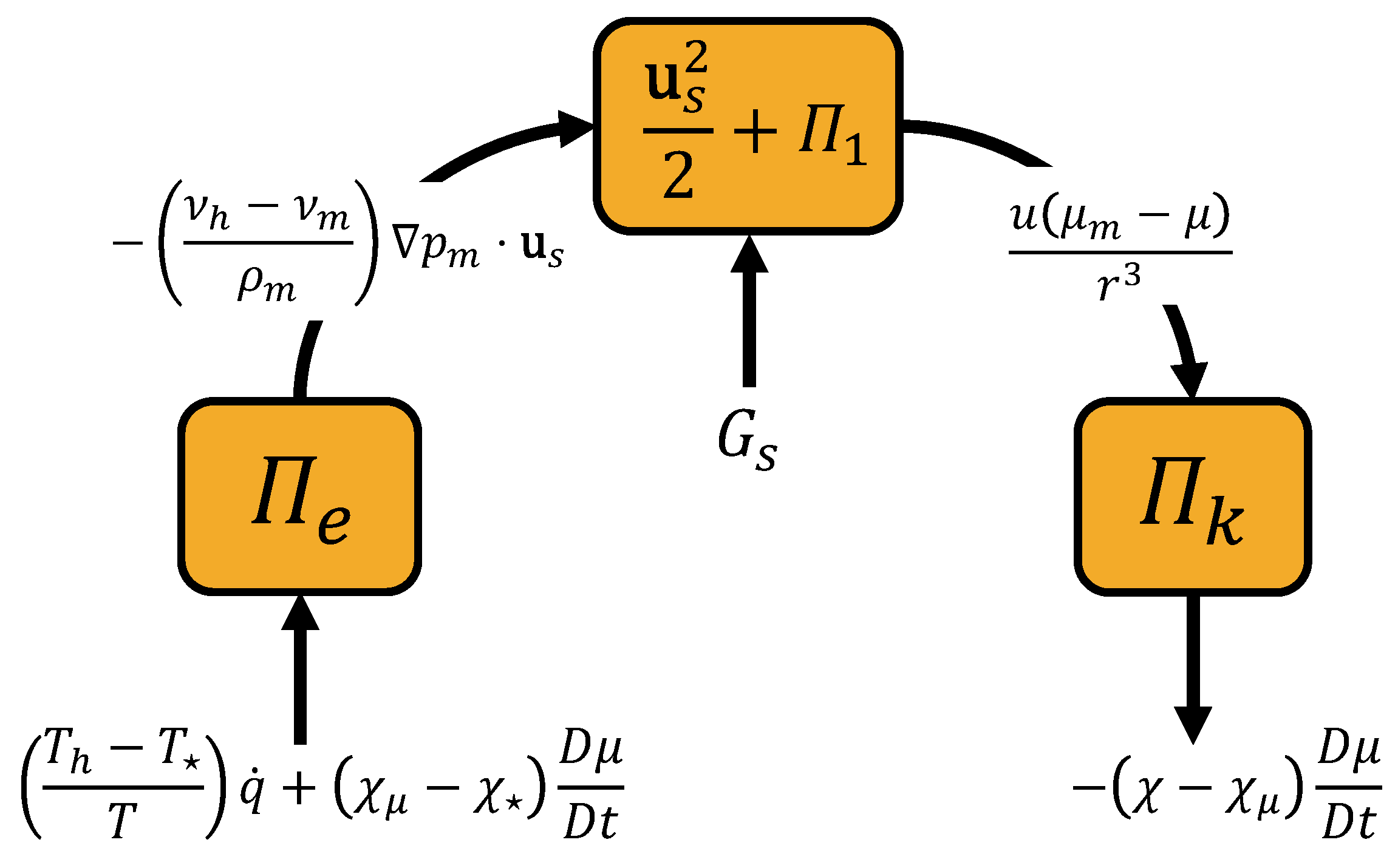
We now regard the azimuthal circulation as the sum of balanced and unbalanced parts $v=v_{★}+v^{″}$ (Lagrangian viewpoint) or $v=v_m+v^{\prime }$ (Eulerian viewpoint). In this view, the observed intensification of v may a priori be due to the intensification of either $v_m$ or $v^{\prime }$ (equivalently $v_{★}$ or $v^{″}$) or both, depending on how $v_m$ is defined. Because there is some freedom in the specification of $v_m$ in the present framework (for instance, it could be imposed to be time independent), we first discuss the case where the intensification of v may be primarily attributed to that of $v^{\prime }$ (restricting ourselves to the Eulerian viewpoint in the following). Evidence that such a case is relevant for the understanding of actual TC intensification is provided by the study of Bui et al. [27], which suggests that the degree of unbalance of TCs is likely significant, especially in the boundary layer. Now, because $v^{\prime }=v-v_m=(M-M_m)/r=(\mu -{\mu }_m)/\left(r(M+M_m)\right)$, any increase in $v^{\prime }$ must result from the creation of a positive anomaly ${\mu }^{\prime }=\mu -{\mu }_m>0$ and hence from an increase in the mechanical energy reservoir ${\Pi }_k$, the only one that increases when $|\mu -{\mu }_m|$ increases.

Prior to discussing energetics, it is useful to first discuss the forces at work in the system, as this is what is most helpful to establish causal relationships. To that end, let us consider the form of the momentum equation for the secondary circulation ${\mathbf{u}}_s$ that makes apparent the role of the generalised inertial/buoyancy force ${\mathbf{b}}_e$, viz.,

$${\displaystyle \frac{D{\mathbf{u}}_s}{Dt}}={\mathbf{b}}_e-{\displaystyle \frac{1}{\rho }}\nabla p^{\prime }-{\nu }^{\prime }\nabla p_m+{\mathbf{D}}_s,$$

(65)

where from (52), the radial and vertical components of ${\mathbf{b}}_e$ may be written explicitly as follows:

$$b_e^{\left(r\right)}=-({\nu }_h-{\nu }_m){\displaystyle \frac{\partial p_m}{\partial r}}+{\displaystyle \frac{(\mu -{\mu }_m)}{r^3}}=-{\rho }_m({\nu }_h-{\nu }_m)\left(f+{\displaystyle \frac{v_m}{r}}\right)v_m+{\displaystyle \frac{(\mu -{\mu }_m)}{r^3}},$$

(66)

$$b_e^{\left(z\right)}=-({\nu }_h-{\nu }_m){\displaystyle \frac{\partial p_m}{\partial z}}={\rho }_{m}g({\nu }_h-{\nu }_m).$$

(67)

One of the expected advantages of introducing a non-resting reference state is to minimise the role of $\nabla p^{\prime }$ in (65) and hence to maximise the ability of ${\mathbf{b}}_e$ to predict the actual acceleration $D{\mathbf{u}}_s/Dt$. Assuming this to be the case, and recalling that $(\mu -{\mu }_m)/r^3>0$, Equation (66) shows that a necessary condition for the radial component of ${\mathbf{b}}_e$ to point towards the centre of the cyclone is that the fluid parcels are positively buoyant,

$${\nu }_h-{\nu }_m>0,$$

(68)

in which case, (67) shows that $b_e^{\left(z\right)}$ will also point upward, as is expected physically. By definition, ${\nu }_h=\nu (\eta ,p_m(r,z))$ and ${\nu }_m=\nu ({\eta }_m(r,z),p_m(r,z))$ so that

$${\nu }_h-{\nu }_m\approx \Gamma (\eta (r,z,t)-{\eta }_m(r,z))$$

(69)

is proportional to the local entropy anomaly ${\eta }^{\prime }=\eta -{\eta }_m$ (we have neglected the time variation of the reference variables, but these can be retained if desired). Since $\Gamma >0$ in general, the creation of a positive specific volume anomaly requires a sustained diabatic source of entropy to increase $\eta$. As discussed by Smith et al. [22], whether (68) is satisfied depends critically on the choice of reference state used to define buoyancy. For instance, Brown [28] found such a condition to be met for buoyancy defined relative to a relatively elaborate reference vortex state, even including some degree of asymmetry. However, Zhang et al. [29] found the parcels to be negatively buoyant for buoyancy defined relative to a rest state, the desired upward acceleration then being entirely provided by the pressure gradient term $\nabla p^{\prime }$.

Even if (68) holds, it is not sufficient to ensure that $b_e^{\left(r\right)}$ is negative. Indeed, because $(\mu -{\mu }_m)/r^3>0$, (66) imposes a further constraint on the magnitude of positive buoyancy anomalies, namely

$${\nu }_h-{\nu }_m>{\left[{\rho }_m\left(f+{\displaystyle \frac{v_m}{r}}\right)v_m\right]}^{-1}{\displaystyle \frac{\mu -{\mu }_m}{r^3}}.$$

(70)

If specific volume anomalies ${\nu }_h-{\nu }_m$ are bounded, as must be the case in reality, (70) appears to impose an upper limit on the maximum angular momentum anomalies $\mu -{\mu }_m$ and hence on the maximum intensity that the vortex can reach. This limit is a priori different from the maximum potential intensity (MPI) predicted by Emanuel [1] (see Emanuel [30] for a recent review on this topic and wider TC research), which is reached when the production of available energy by surface enthalpy fluxes balances the dissipation by surface friction in the region of maximum winds. Whether such a condition could account for why the intensity of many observed TCs remains significantly below their theoretical maximum intensity [31] is left for future study.

4.3. Energy Cycle

The generalised buoyancy/inertial force ${\mathbf{b}}_e$ and other forces that drive the secondary circulation do work and cause energy transfers between the different existing energy reservoirs, for which sources and sinks must exist in order for the system to achieve a steady state. In the following, we discuss the energy cycle associated with an intensifying cyclonic vortex whose intensification is dominated by the intensification of $v^{\prime }$. To that end, we find that the simplest and most economical description of the local energy cycle is one based on separate evolution equations for the following: the sum of the kinetic energy of the secondary circulation plus the AAE, ${\mathbf{u}}_s^2/2+{\Pi }_1$; the eddy slantwise APE ${\Pi }_e$; and the eddy mechanical energy ${\Pi }_k$. This leads to the following set of equations:

$$\rho {\displaystyle \frac{D}{Dt}}\left({\displaystyle \frac{{\mathbf{u}}_s^2}{2}}+{\Pi }_1\right)+\nabla ·\left(p^{\prime }{\mathbf{u}}_s\right)=\rho ({\mathbf{b}}_e^T·{\mathbf{u}}_s+{\mathbf{b}}_e^M·{\mathbf{u}}_s)+\rho G_s,$$

(71)

$$G_s=\left({\displaystyle \frac{T-T_h}{T}}\right)\dot{q}+{\nu }^{\prime }\left({\displaystyle \frac{\partial p_m}{\partial t}}+{\mathbf{u}}_s·\nabla p_m\right),$$

(72)

$${\displaystyle \frac{D{\Pi }_e}{Dt}}=-{\mathbf{b}}_e^T·{\mathbf{u}}_s+\left({\displaystyle \frac{T_h-T_{★}}{T}}\right)\dot{q}+({\chi }_{\mu }-{\chi }_{★}){\displaystyle \frac{D\mu }{Dt}}+{\nu }_h{\displaystyle \frac{\partial p_m}{\partial t}}-{\nu }_{★}{\displaystyle \frac{\partial p_{★}}{\partial t}},$$

(73)

$${\displaystyle \frac{D{\Pi }_k}{Dt}}=-{\mathbf{b}}_e^M·{\mathbf{u}}_s+\left(\chi -{\chi }_{\mu }\right){\displaystyle \frac{D\mu }{Dt}}.$$

(74)

For an intensifying vortex resulting from an increase in $v^{\prime }$, we established in the previous section that ${\nu }_h-{\nu }_m>0$ and $\mu -{\mu }_m>0$. The implications for the work against the generalised inertial and buoyancy forces ${\mathbf{b}}_e^T$ and ${\mathbf{b}}_e^M$ by the secondary circulation are

$$-{\mathbf{b}}_e^M·{\mathbf{u}}_s=(\mu -{\mu }_m)\nabla \chi ·{\mathbf{u}}_s=-{\displaystyle \frac{u(\mu -{\mu }_m)}{r^3}}>0,$$

(75)

$$-{\mathbf{b}}_e^T·{\mathbf{u}}_s=({\nu }_h-{\nu }_m)\nabla p_m·{\mathbf{u}}_s=({\nu }_h-{\nu }_m)\left[u{\displaystyle \frac{\partial p_m}{\partial r}}-{\rho }_{m}gw\right]<0.$$

(76)

The sign of such energy conversions suggests that the flow of energy follows the paths

$${\Pi }_e\to {\displaystyle \frac{{\mathbf{u}}_s^2}{2}}+{\Pi }_1\to {\Pi }_k,$$

(77)

as illustrated in Figure 4. If we neglect the terms related to the time dependence, the following term needs to be positive

$$\left({\displaystyle \frac{T_h-T_{★}}{T}}\right)\dot{q}+({\chi }_{\mu }-{\chi }_{★}){\displaystyle \frac{D\mu }{Dt}}>0.$$

(78)

If $D\mu /Dt<0$ acts as a retarding effect, Figure 2 shows that $(r_{★}-r_{\mu })>0$ and hence that $({\chi }_{\mu }-{\chi }_{★})>0$, suggesting that the sink of angular momentum is of the wrong sign. Therefore, for (78) to act as a source term, the diabatic term must be positive and larger than the term proportional to the angular momentum sink term, viz.,

$$\left({\displaystyle \frac{T_h-T_{★}}{T}}\right)\dot{q}>\left|({\chi }_{\mu }-{\chi }_{★}){\displaystyle \frac{D\mu }{Dt}}\right|>0.$$

(79)

By definition, $T_h=T(\eta ,p_m)$ and $T_{★}=T(\eta ,p_{★})$, so again from Figure 2, $p_m-p_{★}>0$ and therefore $T_h-T_{★}>0$. Now, if we regard $p_m={\widehat{p}}_m({\eta }_m,{\mu }_m)$ as a function of the reference entropy and squared angular momentum, we have

$${\displaystyle \frac{(T_h-T_{★})}{T}}\approx {\displaystyle \frac{1}{T}}{\displaystyle \frac{\partial T}{\partial p}}(p_m-p_{★})\approx -{\displaystyle \frac{1}{T}}{\displaystyle \frac{\partial T}{\partial p}}\left\{{\displaystyle \frac{\partial {\widehat{p}}_m}{\partial {\eta }_m}}(\eta -{\eta }_m)+{\displaystyle \frac{\partial {\widehat{p}}_m}{\partial {\mu }_m}}(\mu -{\mu }_m)+\dots \right\}.$$

(80)

Since, in general, pressure varies little with ${\mu }_m$, it follows that the term is dominated by the entropy anomaly, which needs to be positive as $\partial {\widehat{p}}_m/\partial {\eta }_m<0$. For the intensification of $v^{\prime }$ to proceed, a finite amplitude entropy anomaly ${\eta }^{\prime }$ needs to be produced in order to make the thermodynamic efficiency $(T_h-T_{★})/T$ large enough to satisfy the threshold relation (79), consistent with physical intuition.

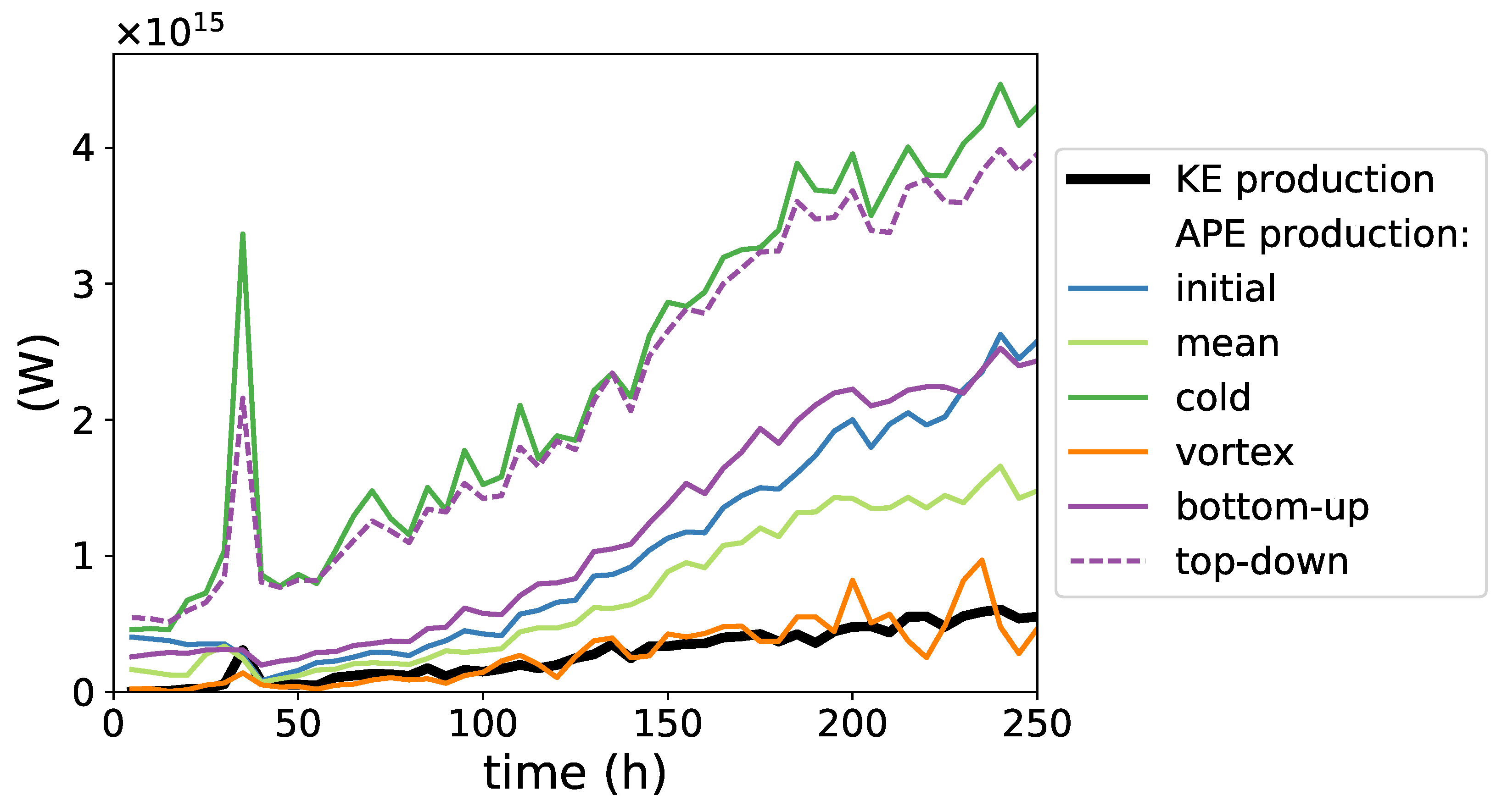
5. Application to Energetics of TC Intensification

5.1. Motivation and Background

One important motivation for the APE-based study of TCs is the quest for a more accurate thermodynamic foundation of Emanuel’s potential intensity (PI) theory. In its most basic form, PI theory is based on balancing the production of energy with dissipation. Specifically, PI theory regards TCs as heat engines whose source of energy can be expressed as a Carnot-type efficiency times the surface enthalpy fluxes, and the dissipation is achieved at the radius of the maximum wind. However, because Carnot theory only provides an upper bound for the energy input of heat engines, PI theory usually greatly overestimates the maximum intensity of TCs. Developments in energetics over the past decade or so, e.g., Tailleux [32], have suggested that APE theory represents a potentially greatly superior approach to the study of heat engines than Carnot theory.

In APE-based studies of TC intensification, the volume-integrated APE and KE budgets may be written as stated in the introduction as

$${\displaystyle \frac{d}{dt}}APE=G_A-C(APE,KE),$$

(81)

$${\displaystyle \frac{d}{dt}}KE=C(APE,KE)-D_K,$$

(82)

where $G_A$ is the net APE production by all possible diabatic terms, including the surface enthalpy fluxes; $C(APE,KE)$ is the reversible conversion between APE and KE; and $D_K$ is the dissipation of kinetic energy. As is well known, the choice of reference state affects the prediction for both the generation term $G_A$ and the storage term $d\left(APE\right)/dt$. The question is whether it is possible to find a reference state such that the associated APE prediction is an accurate predictor of the conversion of APE into KE, in which case

$$C(APE,KE)\approx G_A.$$

(83)

In Wong et al. [12], the authors examined the net generation term for two different constructions of the reference state, one obtained from a top-down sorting of the actual state, the other obtained from a bottom-up sorting. Ways of sorting the atmosphere have been discussed by Harris and Tailleux [11] and Stansifer et al. [10]. Assuming that there is no source of KE other than the APE to KE conversion, one may therefore obtain an alternative to potential intensity theory in the case where a quasi-steady state is reached by balancing the APE production by the dissipation,

$$G_A\approx D_K.$$

(84)

5.2. Numerical Experiment

In local APE theory as developed by Tailleux [17], there is in fact greater freedom in the choice of reference state. Alternative choices are to use the initial sounding, an artificially modified colder sounding, or an isobarically averaged sounding, in addition to the bottom-up and top-down sorted states. Here, we performed an objective test of the suitability of a variety of reference states for understanding tropical cyclone intensification, by assessing the balance between $G_A$ and $C(APE,KE)$ for each reference state in an axisymmetric numerical simulation of a TC.

We used a non-hydrostatic axisymmetric model of Rotunno and Emanuel [33], with modifications to the microphysics by Craig [34,35]. This model simulates the intensification of an existing cyclonic vortex over a slab ocean. The full model setup was identical to the one detailed in Harris et al. [16], in which a method for computing a complete local APE budget was developed, based on using the model’s initialisation sounding as a reference state. This reference state, henceforth referred to as the initial reference state, represents the atmospheric environment outside of the TC. We also tested the top-down and bottom-up reference states based on sorting procedures, as used by Wong et al. [12]. In addition, we introduced the mean reference state, which uses time-varying radial averages of the potential temperature $\theta$ and the water vapour mixing ratio $r_v$ (weighted by the volume represented by each grid point), and the pressure that is in hydrostatic balance with these. Using this reference state rather than the initial state accounts for general heating and moistening across the domain, which alters the environment in which the TC is situated. We additionally tested a cold reference state, computed by taking the initial sounding and subtracting 5 K from $\theta$. The $r_v$ profile was then determined such that the relative humidity profile was the same as in the initial state. Finally, the pressure was adjusted to hydrostatic balance. Computing APE relative to a much colder environment than the one inhabited by the model TC eliminated discontinuities in APE density of the kind found by Harris et al. [16].

Finally, in addition to these non-radially-varying reference states, we tested the vortex reference state, defined by a vortex in thermal wind balance. At each time t, the azimuthal wind speed of the reference vortex was set as the azimuthal wind field from the model, $v_0(r,z,t)=v(r,z,t)$. The thermodynamic fields that held this vortex in hydrostatic and gradient wind balance were then found using the method of Nolan and Montgomery [36]: iterating between integrating inwards to gradient wind balance and adjusting vertically to hydrostatic balance, the thermodynamic fields converged to a reference state determined by $v_0$, ${\theta }_{v_0}$ and ${\Pi }_0$. A decomposition into ${\theta }_0$ and $r_{v_0}$ was required in order to continue using the model’s approximation for buoyancy; it was assumed that $r_{v_0}=r_v$ and then ${\theta }_0$ was calculated from this. This decomposition is non-unique, but the overall results of the APE calculations were found to be insensitive to choosing a different reference mixing ratio, for example using the initialisation sounding value of $r_v$ as $r_{v_0}$.

For the non-radially-varying reference states, the components of the APE budget were calculated according to the method of Harris et al. [16], lifting air parcels vertically to their level of neutral buoyancy (LNB). Using the vortex reference state necessitates accounting for both the radial and vertical motion of each parcel until it reaches its LNB. This was achieved by introducing the angular momentum M as an additional conserved variable, as was performed by Andrews [15] and Codoban and Shepherd [14] when using an axisymmetric vortex as a reference state.

The APE density of a moist air parcel with respect to the vortex reference state was therefore computed by lifting it reversibly and adiabatically along a surface of constant angular momentum until it reached an LNB. Unlike the method used with the profiles that vary in the vertical only, this approach uses information about the trajectory the parcel is expected to follow in the TC. The full numerical discretisation used to lift parcels along surfaces of constant angular momentum to their LNB, along with the model equations for $G_A$ and $C(APE,KE)$ is included in Appendix C.

Our metric for the suitability of a reference state was that the diabatic production of APE (relative to this reference state) should be directly linked to the generation of kinetic energy (which is independent of reference state), and thus to the intensification of the TC. Only the positive parts of the APE production and the kinetic energy production rates were compared, rather than their net production rates. This was done at the parcel level: we integrated the APE production rate over all air parcels in the model for which the APE production was positive. Different diabatic processes may have competing effects on the APE production within the parcel, but its overall APE production must be positive. Similarly, the kinetic energy production rate is integrated over those parcels for which the kinetic energy production is positive. For brevity, these integrals will be referred to as simply the rates of “APE production” and “kinetic energy production”, but it should be understood that they only include the positive contributions to the production. The positive production rates were studied because there is a direct causal link between the (positive) APE production and (positive) kinetic energy production, which does not hold for the dissipation rates. The consideration of only the positive APE production is somewhat analogous to the consideration of only the positive heat input when defining the Carnot efficiency of a heat engine, rather than the net heat input.

Figure 5 compares the rate of kinetic energy production, which is independent of reference state, to the rate of APE production computed using each of the reference states, over the intensification of the TC in the axisymmetric model. The poorest estimation of the kinetic energy production was given by the APE production relative to the cold reference state. This is because when the potential temperature of the reference state is decreased, it no longer resembles the environment that the cyclone actually inhabits, and so the APE production loses physical meaning for the intensification. Measured relative to the cold reference state, almost all parcels below the tropopause will be buoyant; however, this large-scale positive “buoyancy” is not associated with upward vertical motion of all parcels, and so the notional reference heights are mostly not achieved, so most of the APE produced by diabatic processes does not contribute to the generation of kinetic energy.

The sorting-based reference states (top-down and bottom-up) performed worse than the initial or mean reference states. These results indicate that the sorting procedures are releasing too much APE, even in the case of bottom-up sorting, which was specifically intended to limit the APE release to realistic levels [12]. The sorted states were also far more computationally expensive to obtain (taking longer than the model run itself). Therefore, it is preferable to use an environmental reference state to study local APE rather than the sorting methods of Wong et al. [12], although it is possible that other sorting methods could be designed that would perform better.

The mean profile reference state yielded a much closer match than the initial sounding to the kinetic energy production towards the end of the model run. Allowing the reference state to vary with time accounted for general heating and moistening in the domain, which altered the environment experienced by the cyclone. Therefore, using the mean state appears to be preferable to using the initial state.

However, the best predictor of the kinetic energy production for this model run was the vortex reference state, by a substantial margin. Using a reference state that is as close as possible to the actual model state minimised the stored available elastic energy and APE density, and therefore yielded the most direct correspondence between the production of APE and the production of kinetic energy. If a direct link between APE production and kinetic energy production is to be drawn, these results show that accounting for the balanced dynamical structure of the TC is essential. The kinetic energy generation can be entirely explained in this case by the unbalanced part of the flow. A reference state based on a vortex in gradient wind balance allows the production of APE by diabatic processes to be directly linked to the generation of kinetic energy in the TC.

6. Summary and Conclusions

In this paper, we extended the Tailleux [17] local theory of APE to account for momentum constraints for axisymmetric vortex motions in a dry compressible atmosphere. The theory significantly simplifies and extends previous work by Codoban and Shepherd [13,14], Andrews [15] in a number of ways. Notably, we showed that the available potential energy density can be related to to the work against centrifugal and generalised buoyancy forces.

Although the work was derived for a dry atmosphere, we showed that the theory can be used for APE-based studies of moist TC intensification, as recently developed by Harris et al. [16]. The present results show that APE generation based on a non-resting state is a much more accurate predictor of the APE to KE conversion, suggesting that it is therefore a much more accurate quantifier of the potential energy actually available to the tropical cyclone. Such a result has important potential implications for the development of improved potential intensity theories of tropical cyclones, which will be developed in subsequent studies.

References

1. Emanuel, K.A. An air-sea interaction theory for tropical cyclones. Part I: Steady state maintenance. J. Atmos. Sci. 1986, 43, 585–605. [Google Scholar] [CrossRef]
2. Emanuel, K.A. The Maximum Intensity of Hurricanes. J. Atmos. Sci. 1988, 45, 1143–1155. [Google Scholar] [CrossRef]
3. DeMaria, M.; Kaplan, J. Sea Surface Temperature and the Maximum Intensity of Atlantic Tropical Cyclones. J. Clim. 1994, 7, 1324–1334. [Google Scholar] [CrossRef]
4. Bister, M.; Emanuel, K.A. Dissipative heating and hurricane intensity. Meteorol. Atmos. Phys. 1998, 65, 233–240. [Google Scholar] [CrossRef]
5. Lin, I.I.; Black, P.; Price, J.F.; Yang, C.Y.; Chen, S.S.; Lien, C.C.; Harr, P.; Chi, N.H.; Wu, C.C.; D’Asaro, E.A. An ocean coupling potential intensity index for tropical cyclones. Geophys. Res. Lett. 2013, 40, 1878–1882. [Google Scholar] [CrossRef]
6. Balaguru, K.; Foltz, G.R.; Leung, L.R.; D’Asaro, E.; Emanuel, K.A.; Liu, H.; Zedler, S.E. Dynamic Potential Intensity: An improved representation of the ocean’s impact on tropical cyclones. Geophys. Res. Lett. 2015, 42, 6739–6746. [Google Scholar] [CrossRef]
7. Sabuwala, T.; Gioia, G.; Chakraborty, P. Effect of rainpower on hurricane intensity. Geophys. Res. Lett. 2015, 42, 3024–3029. [Google Scholar] [CrossRef]
8. Pauluis, O.M. The Mean Air Flow as Lagrangian Dynamics Approximation and Its Application to Moist Convection. J. Atmos. Sci. 2016, 73, 4407–4425. [Google Scholar] [CrossRef]
9. Lorenz, E.N. Available potential energy and the maintenance of the general circulation. Tellus 1955, 7, 157–167. [Google Scholar] [CrossRef]
10. Stansifer, E.M.; O’Gorman, P.A.; Holt, J.I. Accurate computation of moist available potential energy with the Munkres algorithm. Q. J. R. Meteorol. Soc. 2017, 143, 288–292. [Google Scholar] [CrossRef]
11. Harris, B.L.; Tailleux, R. Assessment of algorithms for computing moist available potential energy. Q. J. R. Meteorol. Soc. 2018, 144, 1501–1510. [Google Scholar] [CrossRef]
12. Wong, K.C.; Tailleux, R.; Gray, S.L. The computation of reference state and APE production by diabatic processes in an idealized tropical cyclone. Q. J. R. Meteorol. Soc. 2016, 142, 2646–2657. [Google Scholar] [CrossRef]
13. Codoban, S.; Shepherd, T.G. Energetics of a symmetric circulation including momentum constraints. J. Atmos. Sci. 2003, 60, 2019–2028. [Google Scholar] [CrossRef]
14. Codoban, S.; Shepherd, T.G. On the available energy of an axisymmetric vortex. Meteorol. Z. 2006, 15, 401–407. [Google Scholar] [CrossRef]
15. Andrews, D.G. On the available energy density for axisymmetric motions of a compressible stratified fluid. J. Fluid Mech. 2006, 569, 481–492. [Google Scholar] [CrossRef]
16. Harris, B.L.; Tailleux, R.; Holloway, C.E.; Vidale, P.L. A moist available potential energy budget for an axisymmetric tropical cyclone. J. Atmos. Sci. 2022, 79, 2493–2513. [Google Scholar] [CrossRef]
17. Tailleux, R. Local available energetics of multicomponent compressible stratified fluids. J. Fluid Mech. 2018, 842, R1. [Google Scholar] [CrossRef]
18. Novak, L.; Tailleux, R. On the local view of atmospheric available potential energy. J. Atmos. Sci. 2018, 75, 1891–1907. [Google Scholar] [CrossRef]
19. Tailleux, R.; Dubos, T. A simple and transparent method for improving the energetics and thermodynamics of seawater approximations: Static Energy Asymptotics (SEA). Ocean Model. 2024, 188, 102339. [Google Scholar] [CrossRef]
20. Smith, R.K.; Montgomery, M.T.; Kilroy, G. The generation of kinetic energy in tropical cyclones revisited. Q. J. R. Meteorol. Soc. 2018, 144, 1–9. [Google Scholar] [CrossRef]
21. Montgomery, M.T.; Smith, R.K. Paradigms for tropical cyclone intensification. Aust. Meteorol. Oceanogr. J. 2014, 64, 37–66. [Google Scholar] [CrossRef]
22. Smith, R.K.; Montgomery, M.T.; Zhu, H. Buoyancy in tropical cyclones and other rapidly rotating atmospheric vortices. Dyn. Atmos. Ocean 2005, 40, 189–208. [Google Scholar] [CrossRef]
23. Emanuel, K.A. The behavior of a simple hurricane model using a convective scheme based on subcloud-layer entropy equilibrium. J. Atmos. Sci. 1995, 52, 3960–3968. [Google Scholar] [CrossRef]
24. Andrews, D.G. A note on potential energy density in a stratified compressible fluid. J. Fluid Mech. 1981, 107, 227–236. [Google Scholar] [CrossRef]
25. Markowski, P.; Richardson, Y. Mesoscale Meteorology in Midlatitudes; Wiley-Blackwell: Hoboken, NJ, USA, 2010. [Google Scholar]
26. Emanuel, K. Atmospheric Convection; Oxford University Press: Oxford, UK, 1994. [Google Scholar]
27. Bui, H.H.; Smith, R.K.; Montgomery, M.T.; Cheng, P. Balanced and unbalanced aspects of tropical cyclone intensification. Q. J. R. Meteorol. Soc. 2009, 135, 1715–1731. [Google Scholar] [CrossRef]
28. Brown, S.A. A cloud resolving simulation of Hurricane Bob (1991): Storm structure and eyewall buoyancy. Mon. Weather Rev. 2002, 130, 1573–1591. [Google Scholar]
29. Zhang, D.L.; Liu, Y.; Yau, M.K. A multiscale numerical study of Hurricane Andrew (1992). Part III. Dynamically induced vertical motion. Mon. Weather Rev. 2000, 128, 3772–3788. [Google Scholar] [CrossRef]
30. Emanuel, K.A. Chapter 15. 100 years of research in tropical cyclone research. Meteorol. Monogr. 2018, 59, 15.1–15.68. [Google Scholar] [CrossRef]
31. Emanuel, K.A. A statistical analysis of tropical cyclone intensity. Mon. Weather Rev. 2000, 128, 1139–1152. [Google Scholar] [CrossRef]
32. Tailleux, R. Entropy versus APE production: On the buoyancy power input in the oceans energy cycle. Geophys. Res. Lett. 2010, 37, L22603. [Google Scholar] [CrossRef]
33. Rotunno, R.; Emanuel, K. An air-sea interaction theory for tropical cyclones. Part II: Evolutionary study using a nonhydrostatic axisymmetric numerical model. J. Atmos. Sci. 1987, 44, 542–561. [Google Scholar] [CrossRef]
34. Craig, G.C. Radiation and polar lows. Q. J. R. Meteorol. Soc. 1995, 121, 79–94. [Google Scholar] [CrossRef]
35. Craig, G.C. Numerical experiments on radiation and tropical cyclones. Q. J. R. Meteorol. Soc. 1996, 122, 415–422. [Google Scholar] [CrossRef]
36. Nolan, D.S.; Montgomery, M.T. Nonhydrostatic, Three-Dimensional Perturbations to Balanced, Hurricane-like Vortices. Part I: Linearized Formulation, Stability, and Evolution. J. Atmos. Sci. 2002, 59, 2989–3020. [Google Scholar] [CrossRef]
37. Smith, R.K. The surface boundary layer of a hurricane. Tellus A Dyn. Meteorol. Oceanogr. 1968, 20, 473. [Google Scholar] [CrossRef]
38. Bennetts, D.A.; Hoskins, B.J. Conditional symmetric instability—A possible explanation for frontal rainbands. Q. J. R. Meteorol. Soc. 1979, 105, 945–962. [Google Scholar]
39. Emanuel, K.A. The Lagrangian parcel dynamics of moist symmetric instability. J. Atmos. Sci. 1983, 40, 2368–2376. [Google Scholar] [CrossRef]
40. Emanuel, K.A. On assessing local conditional symmetric instability from atmospheric soundings. Mon. Weather Rev. 1983, 111, 2016–2033. [Google Scholar] [CrossRef]
Figure 3. Available energy A e of a perturbed dry air parcel at r = 40   k m , z = 5   k m , in terms of M and η perturbations (top panel) and μ and p perturbations (bottom panel). The grey lines in the bottom panel indicate the horizontal and vertical axes along which Π k and Π e change, respectively, and the grey shading covers points in the space that are not sampled by the chosen perturbations of M and η .
Atmosphere 16 00700 g003
Figure 4. Hypothesised energy pathways associated with the intensification of a cyclonic vortex forced by sources of diabatic heating q ˙ and angular momentum D μ / D t .
Atmosphere 16 00700 g004
Figure 5. Comparison between the positive part of the kinetic energy production rate in the axisymmetric numerical model (thick black line) and the positive production rates of APE with respect to each reference state described in Section 5 (coloured lines).
Atmosphere 16 00700 g005
Disclaimer/Publisher’s Note: The statements, opinions and data contained in all publications are solely those of the individual author(s) and contributor(s) and not of MDPI and/or the editor(s). MDPI and/or the editor(s) disclaim responsibility for any injury to people or property resulting from any ideas, methods, instructions or products referred to in the content.