Article

Source Term Estimation for Puff Releases Using Machine Learning: A Case Study

by
John Bartzis
1,*,
Spyros Andronopoulos
2 and
Ioannis Sakellaris
3
1
Department of Mechanical Engineering, University of Western Macedonia, Active Urban Planning Zone (ZEP), 50100 Kozani, Greece
2
Environmental Research Laboratory, Institute of Nuclear & Radiological Sciences & Technology, Energy & Safety, National Centre for Scientific Research “Demokritos”, 15341 Athens, Greece
3
Atmospheric Chemistry & Innovative Technologies Laboratory (AirTech Lab), Institute of Nuclear & Radiological Sciences & Technology, Energy & Safety, National Centre for Scientific Research “Demokritos”, 15341 Athens, Greece
*
Author to whom correspondence should be addressed.
Atmosphere 2025, 16(6), 697; https://doi.org/10.3390/atmos16060697
Submission received: 29 April 2025 / Revised: 4 June 2025 / Accepted: 6 June 2025 / Published: 10 June 2025
(This article belongs to the Section Atmospheric Techniques, Instruments, and Modeling)

Abstract

Reliable source term prediction for hazardous pollutant puffs in urban microenvironments is challenging, especially for risk management under strict time constraints. Puff movement is highly stochastic due to atmospheric turbulence, intensified by complex urban canopies. This complexity, combined with time limitations, makes advanced computational modeling impractical. A more efficient approach is leveraging past and present data using Machine Learning (ML) techniques. This study proposes an ML-based method, enriched with simplified physical modeling, for source term estimation of unforeseen hazardous air releases in monitored urban areas. The Random Forest Regression, commonly used in meteorology and air quality studies, has been selected. A novel variable selection method is introduced, including the following: (a) a model-derived Exposure Burden Index (EBI) reflecting plume–morphology interactions; (b) a plume travel time indicator; (c) the standard deviation of input variables capturing stochastic behavior; and (d) the total dosage-to-mass released ratio at sensor locations as the target variable. The case study examines JU2003 field experiments involving SF6 puffs released at street level in Oklahoma City’s urban core, a challenging scenario due to the limited number of sensors and historical data. Results demonstrate the approach’s effectiveness, offering a promising, realistic alternative to traditional computationally intensive methods.

1. Introduction

Coping with air pollution and its impact on humans and the environment is of utmost importance. The problem of source predictability and associated exposures, as well as timely response under any real circumstances, lies at the heart of the associated challenges. The significant progress in the fields of Computational Fluid Dynamics (CFD) and computer power in recent years can be considered as essential in successfully addressing such a problem. However, it must be kept in mind that the wind flows are stochastic in nature, the associated pollutant sources could be variable in time and/or space, and the application sites could be geometrically complex, such as the urban microenvironments. In such cases advanced CFD modeling with inevitable high computational demands is needed, which can be prohibitive if the requested assessment time has to be limited. The latter is often required when we have to deal with risk management matters. Looking for simpler but reliable approaches in the literature, methodologies based on CFD RANS (Reynolds-averaged Navier–Stokes) modeling seem to have become the most attractive for complex urban environments. However, even for such simplified models, their direct use often requires excessive CPU times, often failing to meet the time constraints needed. Another way forward is to seek data-driven methodologies that exploit past and present relevant data and can contribute towards reducing the time as well as resources for delivering the required output. Looking for such methodologies, the ones based on Artificial Intelligence (AI) have been mainly targeted. The exploitation of Machine Learning (ML) in addressing wind flow and pollutant dispersion has shown rapid development in recent years [1]. The challenge here is how we can hybridize data-driven and first-principal approaches in fluid mechanics [2] to deliver answers with accepted reliability. An extended experience has been gained with Physics-Informed Neural Networks (PINNs) (e.g., [3]). In general, any adopted methodology is often application dependent, meeting the associated problem constraints, which is not always straightforward [4]. Narrowing the subject to the source term estimation, ML methodologies have been applied mainly for continuous releases (e.g., [5,6]). However, to the best of our knowledge, there are no applications concerning puff releases.
It should be clarified here that the present study we are dealing with is the source term estimation of an instantaneous hazardous air release within a monitored urban microenvironment. This problem poses additional difficulties. More specifically, the pollutant released within a second will develop a puff whose movement is strongly stochastic due to ambient air turbulence and therefore quite sensitive to wind fluctuations. Thus, this puff is interacting with the complex urban canopy, leading to pathways that can enter quite different street canyons depending on the precise moment of the release [7]. The straightforward approach for the source quantification is to use advanced CFD models such as DNS or LES, which is prohibitive due to the associated modeling complexity and high computational times. The compromise is to use CFD RANS models, expecting answers with higher uncertainties, which are able to resolve the urban structures’ complexities, but a direct use cannot meet the time constraints since the needed computational time is still quite high. It is reminded that for the risk management team, the operator on duty needs to have such a source estimation in time and most probably within a few minutes. A way forward is to limit the needed number of the necessary simulations by applying wind speed scaling (e.g., [8]). A novel approach with the ambition to offer reliable answers and meet the required time constraints has been successfully developed recently [9], but only for continuous releases. Its key approximations are (a) the needed flow and dispersion simulations, which are only steady state and site- not event-specific; they are performed by CFD RANS models and stored properly, and (b) the actual wind flow and exposure patterns during the event, which are based on the above simulations and applying relatively simple wind speed and exposure time scaling with minor CPU requirements. It should be repeated that the above source term estimation includes possible modeling errors due to several approximations, including the RANS concept itself and its numerics, the adopted scaling assumptions, and the urban topography modeling. On the other hand, at the site under consideration, such events, real and/or experimental, might have taken place, and associated data might have been produced and stored. The key question here is how we can benefit from those data with the aid of AI to reduce the abovementioned errors and even reduce the delay time in providing the needed answers to the operator on duty.
Recognizing the fact that the required knowledge for addressing the above problem successfully with such strict time constraints is really lacking today, the main aim of the present study is to try to close this gap by proposing a new approach based on Machine Learning (ML) methodologies. The key novelty lies in proposing a new coherent set of proper variables (features), either observed or modeled, with some of them presented for the first time. Such a set has to take into consideration all the underlying physics, if possible, but in a simple and inclusive way. Such an approach is needed to serve the following two main purposes: (a) provide the operators a reliable but simple method to work with successfully and (b) pave the way for exploring such novel methods in the general area of air quality assessment and probably beyond. The whole approach is presented and demonstrated through a case study in which the source position is known but the total mass released can be unknown and needs to be estimated. Since this is the first attempt, the obtained demonstration results have at least to enhance the credibility of the proposed approach and, consequently, provide validation results and set the basis for its future systematic validation and evaluation effort.

2. Methods

2.1. The Problem and the Case Study

The problem of interest here can be described in more detail as follows: Let us consider a site in an urban microenvironment that has the potential to face a deliberate or accidental short-duration release of a specific hazardous pollutant/agent at a location within the site. The site is continuously monitored (a) by a network of sensors measuring online the pollutant concentration and (b) by a nearby meteorological station providing air data at a location well above the urban canopy. The user demand, once sensor(s) start indicating a release, is to become fast but reliable information on the pollutant mass released. The effort here is to examine how this demand can be fulfilled by applying well-established machine learning algorithms supported by historical and present (online) data.
Since in the present study, the proposed methodology is quite new, a careful stepwise approach seems more appropriate. Thus, the present problem is restricted to cases where the source location and the onset of the release are considered as identifiable and the real unknown is the total mass released. It is also assumed that the pollutant behaves as a passive tracer. The latter approximation is not far from reality in most cases where the density of the pollutant/air mixture does not differ considerably from that of the surrounding unaffected air.
Looking at the literature for extraction of a case study resembling, to a large extent, the above problem, we ended up at the Joint Urban 2003 (JU2003) field experiments [10]. It is noticed that this experiment has been extensively used for dispersion model validation studies (e.g., [11]). A number of instantaneous puffs of sulfur hexafluoride (SF6) tracer gas were released at street level in a built-up urban center (Oklahoma City) in order to provide a high-quality data set on atmospheric dispersion inside an urban area to be used for model validation purposes. One of the JU2003 experiments, the well-studied IOP3 Experiment [11], concerns successive SF6 releases. More specifically, it includes four (4) successive instantaneous near-ground releases of 1 kg each. The releases were carried out on 7 July 2003 at local times (CST) 8:00 (Puff 1), 8:20 (Puff 2), 8:40 (Puff 3), and 9:00 (Puff 4). Following each puff release, measured concentration signals were produced by a number of sensors (placed downstream of the release location according to the incoming wind direction) with 0.5 s resolution. In addition, an anemometer installed 40m above the ground upwind of the city center provided wind data time series with 1 min resolution.
The experimental layout for IOP3 is shown in Figure 1. All sensors providing successful concentration signals have been considered; more specifically, Puff 1 (sensors: s0, s1, s3, s4, and s8), Puff 2 (sensors: s0, s3, and s6), Puff 3 (sensors: s0, s1, s3, s4, s8, and s9), and Puff 4 (sensors: s0, s1, s3, s6, and s8).

2.2. The Methodology

The basic idea here is to use an appropriate, well-established ML algorithm in order to build a regression model trained by a set of appropriate input variables structured from relevant historical and online data to predict online the proposed target variable.
Translating this approach to the selected case study, it is planned to consider the first three (3) puffs (i.e., Puff 1, Puff 2, and Puff 3) as ‘past events’ generating the required historical data for training purposes, whereas the last Puff 4 release is treated as a ‘present’ event’ for prediction and validation purposes. More specifically, the meteorological and sensor observation signals during the Puff 4 event will be exploited to estimate the total mass released, which is assumed unknown.

2.2.1. The ML Algorithm

It should be noted that this study is a novel work focusing on the selection of the right variables for a candidate ML methodology rather than the evaluation of the various ML algorithms. Since our focus here is risk management and online answers, an important selection criterion besides appropriateness is the ability to meet the pressing time constraints and the training data limitations. For example, despite the extended experience with Physics-Informed Neural Networks (PINNs), their enhanced requirements on training data size and CPU times, as well as the need for careful results interpretation and generalization [4], make those methods initially less attractive for the above applications. Looking for other suitable, well-established methodologies, we ended up with the Random Forest Regression [12], which has been widely used in meteorology and in air quality [13]. Random Forest (RF) algorithms refer to ML methods consisting of an ensemble of decision trees (forest) that are able to capture complex and non-linear relationships between predictor variables [14]. It is noted that in a number of applications, RF has been selected as the preferable approach [15].

2.2.2. The Selected Variables

The data set for the RF algorithm, consisting of the target and associated input variables, are given for each sensor.
The Target
Following the conceptual approach developed by Bartzis et al. [8], we are looking for the relationship between the measured total dosage (D) at a specific sensor and the total mass released (QT).
It is reminded that the measured sensor concentration signal c(t) can be integrated over time to produce the sensor total dosage (D) defined as follows:
D = 0 c t   d t
In practice, the integration is performed between the puff arrival and departure times at the sensor. It is assumed that the pollutant background concentration is zero. Otherwise, any background concentration needs to be subtracted.
Thus, it is proposed that the target for the ML algorithm be the D/QT ratio at each sensor. It should be underlined that the great advantage of quantifying such a parameter is that it simplifies the problem considerably not only in terms of modeling but also in terms of observation. The time resolution of the concentration signal is more dictated by the dosage accuracy than the signal’s detailed description. It is also important that it can be exploited on an equal basis for both forward and inverse problems, i.e., (a) if we know the source, the dosages can be estimated, and (b) if we know the dosages, the associated source can be estimated.
The Input Variables
The path that the pollutant cloud follows and the time that it takes to reach the sensor location depend primarily on the surrounding atmospheric conditions and the site morphology in between the release location and the sensor. On the other hand, the transport mechanism is fully stochastic in nature. It is noted that the material released is carried out by air turbulent eddies with integral time scales of the order of a minute, keeping the stochastic behavior even for time averages over 10 min. It is noted that in the present case study, the releases last on the order of 1 s or less, and the whole phenomenon has already finished within those 10 min. Therefore, when deciding on an input variable related directly or indirectly to wind, some information on the variable statistics needs to be included. Taking into consideration the pioneering character of the present approach and the need to keep things as simple as possible, we have decided to consider only the first two statistical moments, i.e., the mean and standard deviation.
It should be underlined here that the use of statistical moments to describe a stochastic variable besides its mean value allows for obtaining insight into the statistical behavior of the variable, avoiding the complexity of the direct use of the associated pdf (probability density function). The use of higher moments has already been considered with success in the past (e.g., [16]). In the present work, since simplicity is a top priority, it was decided to proceed with caution, including, at least at this pioneering stage, the first and second moments. In fact, the obtained results did not indicate a need that we should go further.
Concerning the atmospheric conditions, the upwind speed and wind direction are expected to be critically affecting the pollutant dispersion in air. Other atmospheric parameters could play a role, especially in cases where the atmospheric stability is non-neutral. In this case, the thermal effects might be important. Parameters that can reveal such an effect and can be measured online are the air temperature and humidity and the solar irradiation. It is noted that the urban canopy enhances the generation of air turbulence, leading the phenomena towards neutrality and reducing the importance of the latter parameters. For the present case study, the wind speed and wind direction provided by the anemometer online during the event are considered as the first input variables.
Concerning the site morphology, one could think of variables related to the site topography. However, in an urban microenvironment with a complex canopy, this exercise is not straightforward. Looking at the relative positions of the source vs. the sensors as well as the buildings and streets in between, the morphology effect is expected to be different for different wind patterns. Therefore, looking for variables describing morphology in a more realistic way, the geometry, of course, needs to be present, but what is also important is how this geometry interacts with the atmospheric conditions to guide the pollutant movement from the source towards the sensor. The plausible approach here is to ask for help from models dealing with airflow and dispersion. The prerequisite is that such models can read the ground geometry as detailed as possible. The use of CFD-RANS models seems to be the first good choice to meet such an objective.
Along these lines, a new variable is proposed called the Exposure Burden Index (EBI), defined as follows: let us assume an arbitrary continuous but constant tracer release rate (Q) from the source location under consideration with a given wind pattern. With the aid of an appropriate flow and dispersion model, we can estimate a steady-state concentration (CSM) at the sensor location. Then, for a specific sensor, EBI is given by the following relationship:
E B I = C S M Q
Such a parameter is directly related to the real D/QT from an instantaneous (puff) release [8] and brings up in a relatively simple way the geometry influence and its interaction with the surrounding air with its wind fluctuations, affecting the fate of the real cloud from the source to the sensor.
A rapid methodology to estimate CSM has been recently developed [9], where all necessary details are given. The CSM estimation for the present case study is discussed below.
It should be noticed from the beginning that for a puff release, the event time interval (Tevent), starting with the onset of the release and ending when the cloud ceases to be observed by all sensors, is of relevance. It is noted that we are only interested in what happens within Tevent, and therefore this time interval determines the range of the required parameterization.
Trying to give a brief description, the whole approach to estimate EBI is translated here into the following historical and ‘during-event’ steps:
Historical steps: (i) Based on historical data, the wind direction range (Θrange) is identified and divided into a sufficient number (NΘ) of individual wind directions (Θi, i = 1, …, NΘ); (ii) for each wind direction, one steady-state wind flow and dispersion simulation is performed, preferably by a CFD RANS model, at a single reference (realistic) wind speed (Uref) and a reference (arbitrary) pollutant constant release rate (Qref); and (iii) the simulation normalized concentrations (CSS/Qref) at each sensor location are calculated and stored as a part of the site historical data and are ready to be used during the event. It should be noted that the parameter (CSS/Qref) is usually CPU intensive, but all associated simulations are site-specific and not event-specific; therefore, they are performed once, at the beginning, and then stored to be used during the event.
During-event steps: (i) For each online wind speed (U) and direction (Θ) instrument reading, the CSS/Qref at the measured direction (Θ) is calculated by simple interpolation of the stored simulation concentration data; (ii) the latter is multiplied by Uref/U to obtain EBI.
What is missing up to now is the time dimension, i.e., the time that it takes for the puff to travel from the source to the sensor. In the present approach, the observed time after the puff release taken for the sensor concentration to reach its peak (i.e., Tpeak) has been used as an additional input variable.
Thus, the following input variables have been selected in the present approach: (a) wind speed and wind direction mean and standard deviation measured by the on-site anemometer during Tevent, reflecting the surrounding meteorological conditions; (b) the Exposure Burden Index (EBI) mean and standard deviation, as defined above, representing the influence of the site morphology/geometry on the plume dispersion; and (c) the time of the measured peak concentration, as a variable representing the travel time of the puff from the release location to the sensor. Concerning the target variable, the proposed parameter is the D/QT ratio, which has the additional advantage of the unified approach of the forward and inverse problem as explained above.
In summary, the present approach has started by having a completely fresh look at how to select the proper set of variables for the ML methodologies able to provide the needed answers to the problem under study. New ideas have been presented on the subject. More specifically, (a) all selected input variables with stochastic behavior have been introduced by both their mean and standard deviation, obtained from the respective detailed observed or modeled signals during the event. (b) The interaction of ground morphology and puff movement is represented by a single, completely new model-derived parameter, the sensor Exposure Burden Index (EBI), and (c) the puff travel time from the source to the sensor has also been considered by the travel time indicator (Tpeak) variable. On the other hand, the selection of the sensor-normalized dosage D/QT is not only introducing the decisive problem of simplicity but also setting both the forward and inverse problems on equal footing. Concerning time constraints, the required CPU time for obtaining the expected answers during the event is marginal. The specific variable selection also facilitates the use of relatively simple and less CPU-intensive ML algorithms. In addition, the proposed concept has been built on principles derived from physical laws and is therefore easily expandable to a variety of applications dealing with the general problem of air quality assessment, especially in complex terrains such as urban ones.

3. The Case Study Application and Results

3.1. The Variables

Looking at the IOP3 experiment concentration signals, it seems that the whole event (i.e., the cloud passage) has taken place within 10 min. Therefore, in order to prepare the abovementioned input variables, only the online observation data within this time range are utilized. In Figure 2 and Figure 3, the mean and standard deviation of the anemometer wind speed and direction, respectively, during Tevent = 10 min for each puff are presented.
There are minor variations from puff to puff. More specifically, the mean wind speeds vary from 5.7 to 7.9 m/s, whereas the mean wind directions vary from 201.8 to 207.8 deg. The standard deviations compared to mean values vary from 16.5 to 20% for speed and 1 to 4% for direction.
To assess to what degree the wind direction variations affect the exposure patterns, in Figure 4 the total dosages (D/QT) for each puff and each sensor are presented. Despite the minor variations of the wind, we can see significant D variations from puff to puff even at the same sensor. This underlines the significant effect of the stochastic behavior of the puff movement within the urban canopy.
The significant effect on stochasticity can be seen also in Figure 5, showing the puffs’ Tpeak at each sensor.
Concerning the EBI estimation, the methodology described in “The Input Variables” Section has been followed. The flow and dispersion offline simulations have been carried out by the CFD RANS code ADREA-HF [17,18,19,20], which has been extensively used for such studies in the past. For the air turbulence closure, the standard k-ε turbulence closure has been utilized. The computational domain horizontal dimensions are 1600 × 1400 m2 in the west–east and south–north directions, respectively (encompassing the Oklahoma City center where JU2003 and, in particular, the IOP3 experiment took place), and 682 m in the vertical direction. Further details are given in [21]. Concerning the grid resolution, a uniform horizontal grid of 5 × 5 m2 and a vertical non-uniform grid with a minimum size near the ground of 1 m have been taken. For the inlet wind speed boundary condition, a one-dimensional (in the vertical direction) wind speed profile calculation is performed, setting a wind speed of 10 ms−1 at the domain top (682 m). The reference release rate is taken as Qref = 1 kg s−1. Given the above boundary conditions, simulations have been performed for 15 wind directions between 191° and 218°, with a 2° interval. The simulations’ normalized concentrations (CSS/Qref) at each sensor are gathered and stored as a part of the site’s historical data and are ready to be used during the event.
Coming to the actual puff releases, all the anemometer individual online readings within Tevent are considered, and the individual EBIs are estimated for each wind speed–direction measured during the Tevent of each puff and for each sensor, as explained in “The Input Variables” Section. From the obtained individual values, the EBI mean value and standard deviation for each puff and sensor are estimated. The results are illustrated in Figure 6. The phenomenon of stochastic behavior is more visible here, as indicated by the relatively large values of the standard deviations, often reaching the corresponding mean values.
Summarizing, the following input variables have been selected for the present case study: (a) wind speed and wind direction mean and standard deviation measured by the on-site anemometer during Tevent, reflecting the surrounding meteorological conditions; (b) the Exposure Burden Index (EBI) mean and standard deviation, as defined above, representing the influence of the site morphology/geometry on the plume dispersion; and (c) the time of the measured peak concentration, as a variable representing the travel time of the puff from the release location to the sensor. Concerning the target variable, the D/QT ratio, a deterministic parameter indicating exposure vs. source relationships at the specific setup.

3.2. The Results

As mentioned above, the RF regressor is trained by all data given for the first three (3) puffs (i.e., Puff 1, Puff 2, and Puff 3). The fourth and last puff (i.e., Puff 4) data are utilized for the problem predictions.
Using the abovementioned variables for the three puffs, an RF Regressor (RFR) has been created using Python 3.9 scikit-learn. Since we are dealing with a rather small amount of data, there was a considerable effort to optimize the RF performance by hyperparameter tuning. It is noticed that the present results have been obtained by the following hyperparameters: Number of Estimators = 50, Maximum Depth = 8, and Minimum Samples Split = 2. The results obtained give good coefficients of determination, i.e., for the training data, R2 = 0.929, whereas for the evaluation data (i.e., Puff 4 data), R2 = 0.766. The importance of the various input variables in shaping up D/QT is illustrated in Figure 7.
It seems that the major input variable is EBI, both in terms of its mean and its variance, followed by Tpeak. This seems quite reasonable, taking into consideration these parameters represent the key underlying physics. The wind parameters’ lower importance can be explained by the fact that the wind effect to a large degree has already been included in the EBI and Tpeak. It should be noted that from the physics point of view, the above results look quite reasonable, revealing the expected significant effect of the atmosphere’s stochastic behavior on the exposure levels at the various locations. This can also be seen as an additional contribution towards defending the specific choice of the present ML algorithm.
The above RF regressor, built from the data of Puff 1, Puff 2, and Puff 3, can now be used to make D/QT predictions for Puff 4. Those predictions compared with observation are shown in Figure 8.
The obtained results seem quite reasonable, supporting the validity of the present concept, especially when considering that the amount of the trained data was rather small.
The predicted D/QT values at each sensor will be used now for the prediction of the total mass released (QT), assuming that corresponding sensor dosages are known. In fact, the D values are estimated by integrating the associated observed sensor concentration signals. The obtained results are shown in Figure 9 as well as in Summary Table 1.
From the five (5) sensors, we produce five (5) Q T values ranging from 0.663 to 1.227, i.e., all within a factor of two (2). The mean value is 0.907 with a rather small standard deviation (sigma = 0.21). Considering that the true value QT = 1.0, the above predicted QT values give a reasonable picture.
The QT values’ differentiation among the sensors could be exploited to have some estimation of the associated uncertainty. A plausible way to go is to consider a reasonable pdf distribution and try to fit the above QT values to this distribution. It is noted that here, we are dealing with stochastic but not purely random phenomena. Therefore, a Gaussian distribution probably is not a good option. Beta functions could be possible options for air pollution-related problems [9,22]. More specifically, a beta function fit has been attempted using SciPy stats in Python. The results in terms of QT beta pdf are shown in Figure 10.

3.3. Study Imitations and the Way Forward

The present case study, with the help of Random Forest methodology, has demonstrated a new, highly promising approach in an application posing important challenges such as a real atmospheric environment and rather limited observation data. Based on the concept-building principles, the results would have been even better if (a) the time resolution of the meteo data was comparable with the pollutant release time duration (i.e., of the order of 1 s, instead of 1 min); (b) the number of sensors able to produce event concentration data was higher; and (c) the number of events for training was higher as well.
Despite those weaknesses, the obtained results were quite good, strengthening the credibility of the proposed approach and giving a strong signal to move forward.
A systematic evaluation/validation would most probably require new experiments. When designing new experiments, there is a need for the following: (a) wind data of time resolution of the order of seconds to better describe the associated stochastic phenomena; (b) a larger amount of training data covering the widest possible range of synoptic wind speeds and directions; (c) an optimized sensor network for measuring concentrations; and (d) extension to non-neutral atmospheric stability conditions.
It should be noted that the present methodology has tried to take into consideration all the key underlying physics but in a simple and inclusive way. Therefore, it has the necessary flexibility to be expandable to the general area of air quality assessment, giving awaiting practical solutions, even at the level of the street canyon spatial resolution when dealing with urban microenvironments.

4. Conclusions

The present study addresses the problem of source term estimation of an unforeseen instantaneous hazardous air release within a monitored urban microenvironment, as detected by the already installed appropriate sensor network. As the first step of this novel methodology, the source location and release time are considered known, and the unknown quantity is the total released mass (QT). The problem itself has inherent difficulties due to the fact that the associated released puff behavior is completely stochastic as it moves through the complex urban canopy. Since such problems are usually related to timely risk management, an additional pressing constraint is the computational time being small enough to allow real-time answers to the user in charge. One way forward is to seek approaches that exploit past and present relevant data using appropriate Machine Learning (ML) methodologies that can contribute towards reducing the time as well as resources for delivering the required output. Looking for well-established but reasonably simple ML methodologies, Random Forest Regression is applied and validated in this work, since it has been widely used in meteorology and in air quality while at the same time is not highly demanding in terms of data size.
The present approach includes important novelties with respect to the definition and selection of the ML variables, such as the new parameters EBI and Tpeak, as well as all standard deviations of the fluctuating variables. The selection of the target variable (D/QT ratio) simplifies the problem considerably and has the additional advantage of the unified approach of the forward and inverse problem.
The new method has been validated by trying to predict the total mass released (QT) concerning the last puff (i.e., Puff 4) of the real-scale IOP3 Experiment taking place during the JU2003 Oklahoma City Campaign.
The results, despite the small size of the training data set, are considered very satisfactory and encourage further research and more extensive validation of the proposed method. Future work is planned to validate the method using more extensive training data sets with wider ranges of incoming wind directions and velocities and including atmospheric data representing effects of other factors such as, e.g., atmospheric stability. Further extension of the methodology is planned for cases where more than one potential release location is identifiable in the spatial domain of interest.

Author Contributions

Conceptualization, J.B.; Methodology, J.B.; Software, J.B., S.A. and I.S.; Formal analysis, J.B. and S.A.; Data curation, S.A. and I.S.; Writing—original draft, J.B.; Writing—review & editing, S.A. and I.S.; Visualization, I.S. All authors have read and agreed to the published version of the manuscript.

Funding

This research received no external funding.

Institutional Review Board Statement

Not applicable.

Informed Consent Statement

Not applicable.

Data Availability Statement

Data set can be made available upon request to the corresponding authors.

Conflicts of Interest

The authors declare no conflicts of interest.

References

  1. Guo, Q.; Ren, M.; Wu, S.; Sun, Y.; Wang, J.; Wang, Q.; Ma, Y.; Song, X.; Chen, Y. Applications of Artificial Intelligence in the Field of Air Pollution: A Bibliometric Analysis. Front. Public Health 2022, 10, 933665. [Google Scholar] [CrossRef] [PubMed]
  2. Brunton, S.L.; Noack, B.R.; Koumoutsakos, P. Machine Learning for Fluid Mechanics. Annu. Rev. Fluid Mech. 2020, 52, 477–508. [Google Scholar] [CrossRef]
  3. Raissi, M.; Perdikaris, P.; Karniadakis, G.E. Physics-Informed Neural Networks: A Deep Learning Framework for Solving Forward and Inverse Problems Involving Nonlinear Partial Differential Equations. J. Comput. Phys. 2019, 378, 686–707. [Google Scholar] [CrossRef]
  4. Farea, A.; Yli-Harja, O.; Emmert-Streib, F. Understanding Physics-Informed Neural Networks: Techniques, Applications, Trends, and Challenges. AI 2024, 5, 1534–1557. [Google Scholar] [CrossRef]
  5. Alessandrini, S.; Meech, S.; Cheng, W.; Rozoff, C.; Kumar, R. Comparing Machine Learning and Inverse Modeling Approaches for the Source Term Estimation. Air Qual. Atmos. Health 2024, 17, 2169–2186. [Google Scholar] [CrossRef]
  6. Wang, R.; Chen, B.; Qiu, S.; Ma, L.; Zhu, Z.; Wang, Y.; Qiu, X. Hazardous Source Estimation Using an Artificial Neural Network, Particle Swarm Optimization and a Simulated Annealing Algorithm. Atmosphere 2018, 9, 119. [Google Scholar] [CrossRef]
  7. Berbekar, E.; Harms, F.; Leitl, B. Dosage-Based Parameters for Characterization of Puff Dispersion Results. J. Hazard. Mater. 2015, 283, 178–185. [Google Scholar] [CrossRef] [PubMed]
  8. Bartzis, J.G.; Sakellaris, I.A.; Efthimiou, G. On Exposure Uncertainty Quantification from Accidental Airborne Point Releases. J. Hazard. Mater. Adv. 2022, 6, 100080. [Google Scholar] [CrossRef]
  9. Bartzis, J.G.; Sakellaris, I.A.; Andronopoulos, S.; Venetsanos, A.; Triantafyllou, A. Towards New Simplified Methodologies on Source Term Estimation and Associated Uncertainties from Accidental Airborne Releases. Build. Environ. 2024, 251, 111222. [Google Scholar] [CrossRef]
  10. Allwine, J.; Leach, M.; Stockham, L.; Shinn, J.; Hosker, R.; Bowers, J.; Pace, J. Overview of Joint Urban 2003: An Atmospheric Dispersion Study in Oklahoma City. In Proceedings of the Symposium on Planning, Nowcasting, and Forecasting in the Urban Zone, Seattle, WA, USA, 12 January 2004. [Google Scholar]
  11. Hernández-Ceballos, M.A.; Hanna, S.; Bianconi, R.; Bellasio, R.; Chang, J.; Mazzola, T.; Andronopoulos, S.; Armand, P.; Benbouta, N.; Čarný, P.; et al. UDINEE: Evaluation of Multiple Models with Data from the JU2003 Puff Releases in Oklahoma City. Part II: Simulation of Puff Parameters. Bound.-Layer Meteorol. 2019, 171, 351–376. [Google Scholar] [CrossRef]
  12. Cutler, A.; Cutler, D.R.; Stevens, J.R. Random Forests. In Ensemble Machine Learning: Methods and Applications; Zhang, C., Ma, Y., Eds.; Springer: New York, NY, USA, 2012; pp. 157–175. ISBN 978-1-4419-9326-7. [Google Scholar]
  13. Balogun, A.-L.; Tella, A.; Baloo, L.; Adebisi, N. A Review of the Inter-Correlation of Climate Change, Air Pollution and Urban Sustainability Using Novel Machine Learning Algorithms and Spatial Information Science. Urban Clim. 2021, 40, 100989. [Google Scholar] [CrossRef]
  14. Gariazzo, C.; Carlino, G.; Silibello, C.; Renzi, M.; Finardi, S.; Pepe, N.; Radice, P.; Forastiere, F.; Michelozzi, P.; Viegi, G.; et al. A Multi-City Air Pollution Population Exposure Study: Combined Use of Chemical-Transport and Random-Forest Models with Dynamic Population Data. Sci. Total Environ. 2020, 724, 138102. [Google Scholar] [CrossRef] [PubMed]
  15. Wang, J.-X.; Wu, J.-L.; Xiao, H. Physics-Informed Machine Learning Approach for Reconstructing Reynolds Stress Modeling Discrepancies Based on DNS Data. Phys. Rev. Fluids 2017, 2, 034603. [Google Scholar] [CrossRef]
  16. Hinder, F.; Brinkrolf, J.; Hammer, B. Feature Selection for Trustworthy Regression Using Higher Moments. In Proceedings of the Artificial Neural Networks and Machine Learning—ICANN 2022; Pimenidis, E., Angelov, P., Jayne, C., Papaleonidas, A., Aydin, M., Eds.; Springer Nature: Cham, Switzerland, 2022; pp. 76–87. [Google Scholar]
  17. Bartzis, J.G.; Varvayanni, M.; Venetsanos, A.; Catsaros, N.; Housiadas, C.; Horsch, G.; Statharas, J.; Amanatidis, G.T.; Megaritou, A.; Konte, K. ADREA-I: A Three-Dimensional Finite Volume Transport Code for Mesoscale Atmospheric Transport (The Cartesian Version) Part I: The Model Description. NCSR Demokritos Demo 1993, 93. [Google Scholar] [CrossRef]
  18. Andronopoulos, S.; Bartzis, J.G.; Würtz, J.; Asimakopoulos, D. Modelling the Effects of Obstacles on the Dispersion of Denser-than-Air Gases. J. Hazard. Mater. 1994, 37, 327–352. [Google Scholar] [CrossRef]
  19. Andronopoulos, S.; Grigoriadis, D.; Robins, A.; Venetsanos, A.; Rafailidis, S.; Bartzis, J.G. Three-Dimensional Modelling of Concentration Fluctuations in Complicated Geometry. Environ. Fluid Mech. 2001, 1, 415–440. [Google Scholar] [CrossRef]
  20. Venetsanos, A.G.; Papanikolaou, E.; Bartzis, J.G. The ADREA-HF CFD Code for Consequence Assessment of Hydrogen Applications. Int. J. Hydrog. Energy 2010, 35, 3908–3918. [Google Scholar] [CrossRef]
  21. Andronopoulos, S.; Bartzis, J.G.; Efthimiou, G.C.; Venetsanos, A.G. Assessment of Puff-Dispersion Variability Through Lagrangian and Eulerian Modelling Based on the JU2003 Campaign. Bound.-Layer Meteorol. 2019, 171, 395–422. [Google Scholar] [CrossRef]
  22. Bartzis, J.G.; Efthimiou, G.C.; Andronopoulos, S. Modelling Short Term Individual Exposure from Airborne Hazardous Releases in Urban Environments. J. Hazard. Mater. 2015, 300, 182–188. [Google Scholar] [CrossRef] [PubMed]
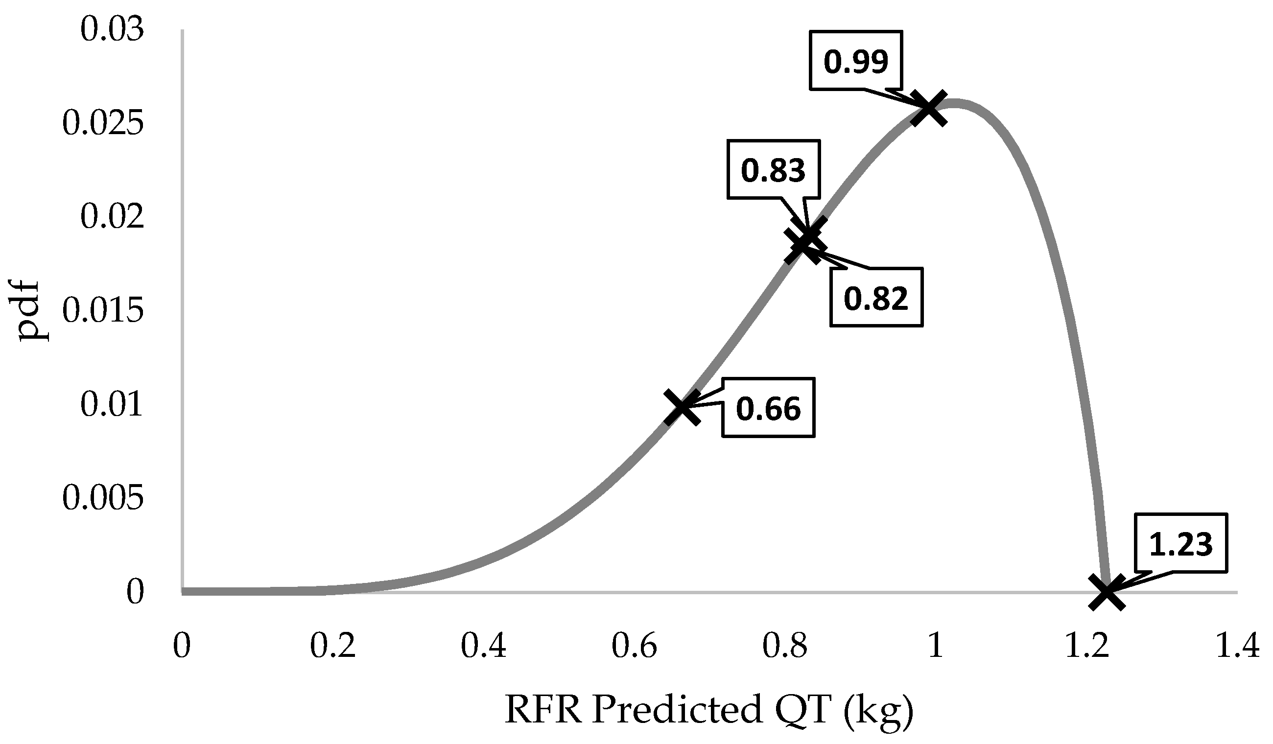
Figure 1. The IOP3 experiment layout: puff release (red) and sensor’s locations (blue).
Atmosphere 16 00697 g001
Figure 2. Anemometer wind speed means and standard deviations for all puffs.
Atmosphere 16 00697 g002
Figure 3. Anemometer wind direction means and standard deviations for all puffs.
Atmosphere 16 00697 g003
Figure 4. Sensors source normalized total dosage for all sensors and the four (4) puffs.
Atmosphere 16 00697 g004
Figure 5. Tpeak values at all sensors and the four (4) puffs.
Atmosphere 16 00697 g005
Figure 6. Sensors EBI means and standard deviations for all puffs.
Atmosphere 16 00697 g006
Figure 7. Input feature importances.
Atmosphere 16 00697 g007
Figure 8. Puff 4: D/QT predictions versus observations.
Atmosphere 16 00697 g008
Figure 9. Puff 4: QT results and predictions per sensor.
Atmosphere 16 00697 g009
Figure 10. Puff 4: QT prediction uncertainty in terms of beta pdf. The numbers refer to the individual predictions of sensors. What is interesting in this figure is the derived pdf mode (i.e., the most likely value) QT = 1.024 (given also in Table 1) is very close to the true value QT = 1.0.
Atmosphere 16 00697 g010
Table 1. Summary of QT predictions (true value is QT = 1.0).
MinMaxMeanSigmaBeta Mode
0.6631.2270.9070.2131.024
Disclaimer/Publisher’s Note: The statements, opinions and data contained in all publications are solely those of the individual author(s) and contributor(s) and not of MDPI and/or the editor(s). MDPI and/or the editor(s) disclaim responsibility for any injury to people or property resulting from any ideas, methods, instructions or products referred to in the content.

