Article

Evaluation of Automated Spread–F (SF) Detection over the Midlatitude Ionosphere

by
Krishnendu Sekhar Paul
1,*,
Trisani Biswas
2,3 and
Haris Haralambous
1,3
1
Frederick Research Center, Nicosia 1035, Cyprus
2
GeoImaging Ltd., Strovolos, Nicosia 2021, Cyprus
3
Department of Electrical and Computer Engineering and Informatics, Frederick University, Nicosia 1036, Cyprus
*
Author to whom correspondence should be addressed.
Atmosphere 2025, 16(6), 642; https://doi.org/10.3390/atmos16060642
Submission received: 16 April 2025 / Revised: 12 May 2025 / Accepted: 23 May 2025 / Published: 25 May 2025

Abstract

:
The present study evaluates an automated Spread–F (SFP) detection algorithm by integrating SF-related (QF, FF) and ionospheric parameters (hmF2, h’F), acting as an indicator for SF events, from SAO Explorer auto-scaled (ARTIST) data, compared to manually identified SF events (SFM) across nine European midlatitude ionospheric stations. The stations were categorized into four latitude sectors to evaluate latitudinal influence in an analysis within the period 2009–2021 from low to high solar activity levels. The results revealed an inverse correlation between solar activity and agreement between SFP and SFM, with stronger agreement during the solar minimum. In the 55°–60° N sector, the SFPSFM match varied from 71% during the solar minimum to 47% during the solar maximum, with overestimation associated with LSTID activity. In the 50°–55° N sector, agreement ranged from 66% to 56%, with overestimation associated with MSTIDs and oblique traces. The 40°–45° N sector exhibited the highest variability (89% to 42%), where Satellite Traces (STs), Multiple Reflected Echoes (MREs), and spread Es led to both over– and underestimations. In the 35°–40° N sector, agreement dropped to 30% during the solar maximum, with wintertime overestimation and summer underestimation significantly characterized by STs, MREs, and Es–layer interference.

1. Introduction

The midlatitude ionosphere is generally less variable than its equatorial and polar counterparts. However, it often exhibits complex dynamics during nighttime, including irregular plasma structures collectively known as midlatitude spread F (SF). These structures can persist from several minutes to hours and are a prominent feature of post-sunset ionospheric variability [1,2,3,4,5,6]. SF events are of considerable importance due to their potential to disrupt essential technologies. They can interfere with high-frequency (HF) radio communications, reduce the accuracy and reliability of satellite-based navigation and positioning systems, and degrade the quality of remote sensing data critical for both scientific research and operational applications [7].
Observational studies have highlighted the key morphological characteristics of SF occurrence, demonstrating its solar, seasonal, and diurnal variability [4,5,6,8]. Nighttime irregularities in the midlatitude F region are primarily driven by spatial and temporal electron density variations, often originating from gravity wave (GW) propagation from the lower atmosphere [9]. These GWs cause vertical displacements in the ionosphere, and as Miller et al. (1997) [10] noted, when coupled with the tilted geomagnetic field at midlatitudes, they create a divergence in global ionospheric currents, which generates localized electric fields. These fields can vary diurnally and potentially initiate plasma instabilities that trigger SF. Several studies [1,11,12] have examined such plasma dynamics, with Bowman (1996) [2] finding an inverse relationship between SF occurrence and solar flux. This anti-correlation is attributed to changes in upper atmospheric neutral particle density (UA–NPD), which significantly influence the amplitude of travelling ionospheric disturbances (TIDs)—the ionospheric signature of GW coupling from the neutral atmosphere into the ionosphere [13]. These TIDs can induce tilts in the F layer, and when their amplitudes are sufficiently large, they can trigger SF formation. Hines (1963) [14] further supported this link by demonstrating that TID amplitudes are regulated by neutral density, thus linking variations in UA–NPD to the prevalence of SF events [2].
SF events, as identified from ionograms, are typically categorized into three types based on the morphology and spatial origin of the echo spread [3,4,12]. Range Spread F (RSF) manifests as horizontally extended, diffuse echoes, usually below 2–2.5 MHz, indicating large-scale plasma irregularities spanning over 10 km and sometimes stretching up to ~1000 km in length [15]. Frequency Spread F (FSF) is characterized by spreading near the F layer’s critical frequency, resulting from vertical scattering by irregularities located near the ionospheric zenith [12]. Mixed Spread F (MSF) exhibits simultaneous spreading in both frequency and range, suggesting the co-occurrence of vertical and horizontal irregularity structures [3,4].
SF occurrence varies significantly with latitude and longitude, as documented in numerous studies [3,5,6,9,16,17,18]. Early investigations by Singleton (1968) [16] and Shimazaki (1962) [19] revealed seasonal, solar, and latitudinal dependencies. More recent work by Paul et al. (2022, 2023) [5,6] demonstrated marked differences in nighttime SF across European midlatitude stations, confirming the complexity of SF geographical distribution. Among the primary drivers of SF is the uplift of the bottom-side F layer (h′F), with RSF events at midlatitudes often linked to such uplifts, similar to equatorial conditions. This was observed by Bowman (1960) [15], attributed to TIDs by Hines (1963) [14], and confirmed by Paul et al. (2018, 2019) [3,4]. FSF, in contrast, has been associated with rises in the F2 layer peak (hmF2). Bowman (1990, 2001) [1,18] distinguished two SF types: Type 1 (pre-midnight, RSF-linked, solar activity–dependent) and Type 2 (post-midnight, FSF-linked, inversely related to solar activity). These classifications were supported by Paul et al. (2019, 2022) [4,5]. FSF typically appears after midnight [3], often coupled with F2 layer uplifts and foF2 fluctuations, even under weak wave conditions [15,20], and has been corroborated by observations over sites like Nicosia and Moscow [5].
Accurate detection and monitoring of SF events are vital for establishing a global understanding of ionospheric irregularities and enhancing prediction capabilities. While the manual interpretation of ionograms remains the most reliable approach due to the ability of trained observers to detect subtle and complex signatures, it is impractical for large-scale, long-term studies because of the labor-intensive and time-consuming nature of SF identification. One major limitation of manual SF identification is the lack of standardized criteria, particularly for FSF. While Hajkowicz (2007) [12] offered some guidelines for detecting RSF, no such detection methods still exist for FSF. Consequently, the accuracy and consistency of manual SF classification largely depend on the expertise and subjectivity of the “scaler”. To address these limitations, automated ionogram processing tools, such as the ARTIST (Automatic Real-Time Ionogram Scaler with True height) algorithm integrated within the SAO Explorer [21], have been developed. ARTIST is widely deployed within the Global Ionospheric Radio Observatory (GIRO) network [22], which consists of over 80 Digisonde stations worldwide. This network has resulted in more than 30 million ionograms from 64 active stations, with 42 providing near-real-time data. The availability of these real-time observations has facilitated the incorporation of ionosonde-derived parameters into empirical models, such as the real-time extension of the International Reference Ionosphere (IRI) [23]. ARTIST in SAO Explorer extracts several parameters as proxies for identifying SF events, including QF (quantifying the average range spread of the F layer, typically associated with RSF), FF (indicating frequency spread, typically associated with FSF), and QE (reflecting spread in the sporadic E layer). These auto-scaled parameters are increasingly used in large-scale statistical analyses and real-time ionospheric monitoring. However, their reliability and accuracy remain subjects of scrutiny. To evaluate the possible accuracy of automated SF detection parameters, Figure 1a,b presents two representative ionograms recorded over Nicosia in 2016. Figure 1a shows an ionogram from 05:07 UT on 14 December 2016, where no SF features were visible upon manual evaluation, yet the auto-scaler inaccurately recorded a QF value of ~10 km, indicating a false positive. Figure 1b provides a consistent detection case: both manual and automated methods correctly identified the SF event at 22:22 UT on 12 June 2016, with elevated QF and FF values (>10 km and >0.2 MHz, respectively), confirming the presence of SF. A more systematic evaluation was carried out by Paul and Haralambous (2025) [24], who conducted a comparative analysis of manual versus automated SF detection over Nicosia for the year 2016. They reported a weak correlation between manually identified RSF events and the QF parameter, with only 14% overlap. A slightly better agreement (26%) was found between FSF and the FF parameter. Furthermore, their study concluded that the QE parameter was largely ineffective in detecting Es layer spread over Nicosia. These findings underscore the limitations of relying solely on ARTIST-derived SF-detection parameters for automated SF detection due to the inherently complex and variable nature of SF formation. It is important to emphasize that our main focus is on the binary detection of SF events—i.e., determining whether an SF occurrence is present or absent—through automated means. To enhance detection reliability, we developed an algorithm that combines ARTIST-derived SF indicators (QF and FF) with ionospheric parameters known to act as indicators or drivers of SF, as established in previous literature.
This study evaluates the accuracy and consistency of an automated SF detection algorithm that integrates SF-derived indicators with ionospheric parameters obtained from ARTIST, by comparing its outputs against manually identified SF occurrences at nine midlatitude ionospheric stations across Europe. The analysis utilizes a comprehensive dataset spanning from 2009 to 2021 and incorporates two key ionospheric parameters that act as key SF drivers—hmF2 uplifts in conjunction with the FF parameter to identify FSF events and h′F fluctuations combined with the QF parameter to detect RSF events—as suggested in earlier studies [1,4,5]. By contrasting automated detections with manually verified events, the study aims to determine the effectiveness of these parameters in reliably identifying SF phenomena. The manuscript is structured into five sections: Section 1 outlines the background and objectives; Section 2 details the data sources; Section 3 presents the analytical method; Section 4 discusses the results; and Section 5 offers a summary and concluding remarks.

2. Data

We analyzed data from nine Digisonde stations located across the European midlatitude ionosphere. The geographic locations of these stations are illustrated in Figure 2, while their precise coordinates and data availability details are presented in Table 1. For a comprehensive assessment and validation of SF events, we utilized nighttime ionogram data spanning a 13–year period from 2009 to 2021 across all selected stations. The temporal resolution of ionogram recordings varied among stations, ranging between 5 and 15 min during the study period. All ionogram data were retrieved from the Digital Ionogram Database (DIDBase), available at https://giro.uml.edu/ionoweb/ (accessed on 4 March 2025) [22].
In addition, to evaluate the automated SF detection method, we employed auto–scaled ionogram data obtained from the FastChar database hosted on the DIDBase platform (https://giro.uml.edu/didbase/scaled.php, accessed on 7 March 2025). These auto–scaled datasets were acquired for the same nine stations and over the same time interval as in the manual analysis. Any anomalies detected during daytime hours were excluded. From the auto-scaled ionograms, we considered four key parameters associated with SF detection, QF, FF, hmF2, and hF, which we have referred to as h’F.
During data acquisition, several data gaps were encountered, resulting in a reduced number of usable records for evaluating the performance of the automated algorithm. In particular, notable data deficiencies were observed for the following stations and years: Chilton (2020), Pruhonice (2009 and 2020), Rome (2017), Athens (2009), and Nicosia (2020 and 2021).
To assess the potential influence of solar activity on the present comparative study, we analyzed yearly average sunspot numbers (SSN) as an indicator of solar variability. The SSN data were obtained from the Solar Influences Data Analysis Center (SIDC), accessible at https://www.sidc.be/SILSO/datafiles (accessed on 11 March 2025).

3. Analysis

3.1. Automated SF Detection

Our primary focus was the evaluation of the automated SF detection exploiting the four detection parameters retrieved from the GIRO portal, as described in the previous section. The GIRO retrospective dataset is based on ARTIST auto-scaling [25]. While ARTIST facilitates automated processing, manually scaled ionograms yield more accurate results, particularly for critical measurements, like hmF2 and h’F. According to Bamford et al. (2008) [26], the discrepancy between manual and auto-scaled values may reach up to 50–100 km or more in extreme cases.
To ensure data integrity in our analysis, we discarded any cases that exhibited the following scaling inconsistencies:
(a) Excessive h’F fluctuations (Δh’F > 200 km), suggesting unstable or erroneous auto–scaling;
(b) FF values exceeding 1 MHz, which may reflect unrealistic frequency spreading events.
To identify potential drivers for RSF events—particularly those associated with sudden uplifts of the bottom-side F layer (as described in [3,4])—we calculated h’F fluctuations (Δh’F) using the second-difference method [27]. In this context, we focused solely on the magnitude of the fluctuations, disregarding the sign, as we aimed at the quantification of the intensity of the variation rather than its direction.
For the purpose of automated SF detection, we established the following criteria based on empirical evidence and insights from prior studies:
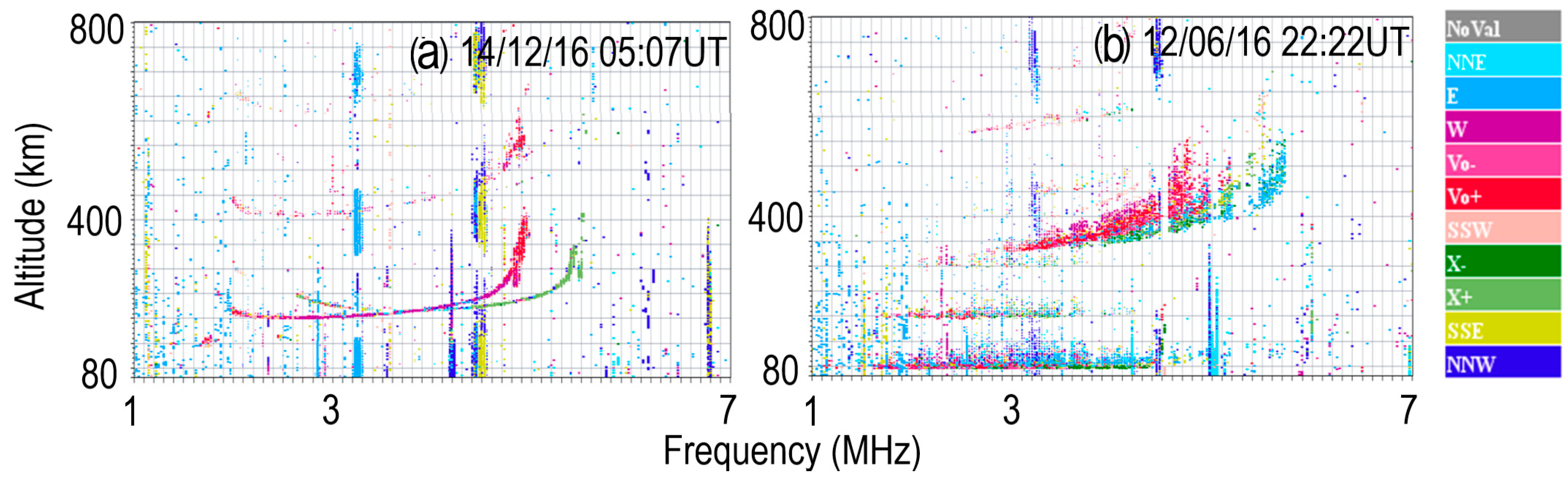
  • QF > 0: This condition indicates the presence of RSF and specifies horizontal spreading in the F layer trace. QF is considered latitude independent and serves as a basic indicator of RSF activity [24].
  • a < Δh′F < 200 km: h′F is a critical parameter, which indicates a sudden F layer uplift as an RSF driver. Δh′F exceeding a threshold value ‘a’ strongly suggests the likelihood of RSF. The value of ‘a’ (in km) is latitude dependent, as SF occurrence depends on latitude. We also apply an upper limit of 100 km to avoid spurious values caused by auto-scaling.
  • hmF2 > b for FF < 1 MHz: hmF2 is commonly linked to FSF formation [1]. Here, we define ‘b’ (in km) as a latitude-dependent threshold, beyond which the probability of FSF increases under the condition that FF remains within realistic limits (FF < 1 MHz).
  • FF > c and FF < 1 MHz, with hmF2 > b: While FF can indicate FSF, not all FF values confirm its presence. According to Paul and Haralambous (2025) [24], some FF values may result from unrelated irregularities. To address this, we calculated a threshold ‘c’ (in MHz), above which FF values pointed to confirmed FSF occurrence, particularly when accompanied by higher hmF2 values (hmF2 > b).
Based on these four conditions, we formulated a latitude-dependent automated SF detection algorithm capable of distinguishing between RSF and FSF events by applying realistic, validated thresholds. While automated SF detection is well-established, most efforts have focused on equatorial regions or confined geographic areas. Scotto et al. (2018) [28] developed an image recognition-based method for automated SF detection using ionograms from Tucumán, enhancing the ability of autoscaling to reject low-quality ionograms and supporting space weather applications. Rao et al. (2022) [29] proposed a technique for the automated detection of Sporadic E and SF events by de-noising and segmenting ionograms, achieving high detection rates (Es: 96.71%, RSF: 89.71%, SSF: 93.39%) using data from a low-latitude station in Hyderabad. Despite their accuracy, these models are limited to equatorial regions and rely heavily on ionogram data, which involves managing large datasets. In contrast, the current work introduces a novel, ionogram-independent algorithm tailored for the midlatitude ionosphere, offering greater versatility and operational efficiency.

3.1.1. Algorithm Used for Automated SF Detection

In the present study, we developed an automated SF detection algorithm based on specific ionospheric parameters and their threshold values, considering both RSF and FSF detection individually. The automated SF occurrence, denoted as SFP, is expressed as a logical combination of the two individual components:
SFP = FSFP + RSFP
Here, RSFP and FSFP represent the automated detection of RSF and FSF, respectively, with the ‘+’ symbol denoting a logical OR operation. From previous studies [1,4,5], we derive expressions for RSFP and FSFP based on the drivers:
FSFP = (c < FF < 1MHz) × (hmF2(n) > b)
RSFP = (QF > 0) × (a < Δh’F(n) < 200 km)
Summarizing the Equations (1)–(3),
SFP = [(c < FF < 1MHz) × (hmF2(n) > b)] + [RSFP = (QF > 0) × (a < Δh’F(n) < 200 km)]
where ‘×’ indicates a logical AND operation, and a, b, and c are threshold values for Δh′F, hmF2, and FF, respectively. These thresholds vary based on latitude (Lat), solar activity (represented by yearly average SSN), and time interval (t), expressed by the function
n = f(Lat, SSN, t)
To address the pronounced latitudinal variation in SF occurrence [3,6], we grouped the nine observational stations (Table 1) into four distinct latitudinal regions using a 5° latitude grid. From each region, one representative station was selected to derive the parameters a, b, and c for the SF detection algorithm. The associated color scheme (depicted in Figure 1 and detailed in Table 1) is consistently used throughout the analysis. Additionally, to account for the role of the solar terminator—a known contributor to SF generation [3,5,6,28]—we adopted specific local nighttime intervals for each latitudinal zone based on a standard solar terminator pattern. The complete information is summarized in Table 2.

3.1.2. Calculation of Threshold Values

To determine the threshold values a, b, and c for the parameters Δh′F, hmF2, and FF, respectively, we employed different approaches tailored to the statistical characteristics and physical behavior of each parameter.

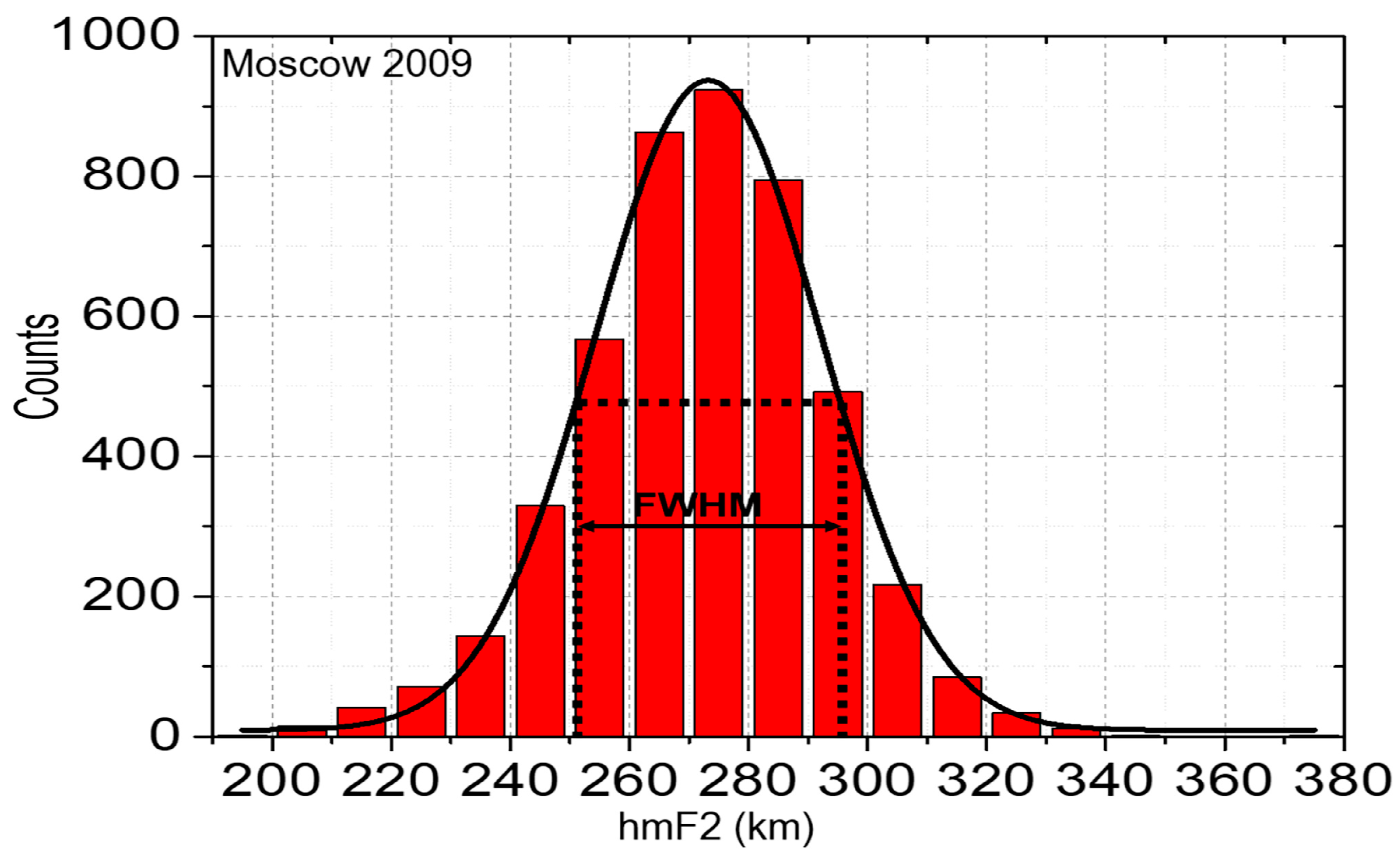
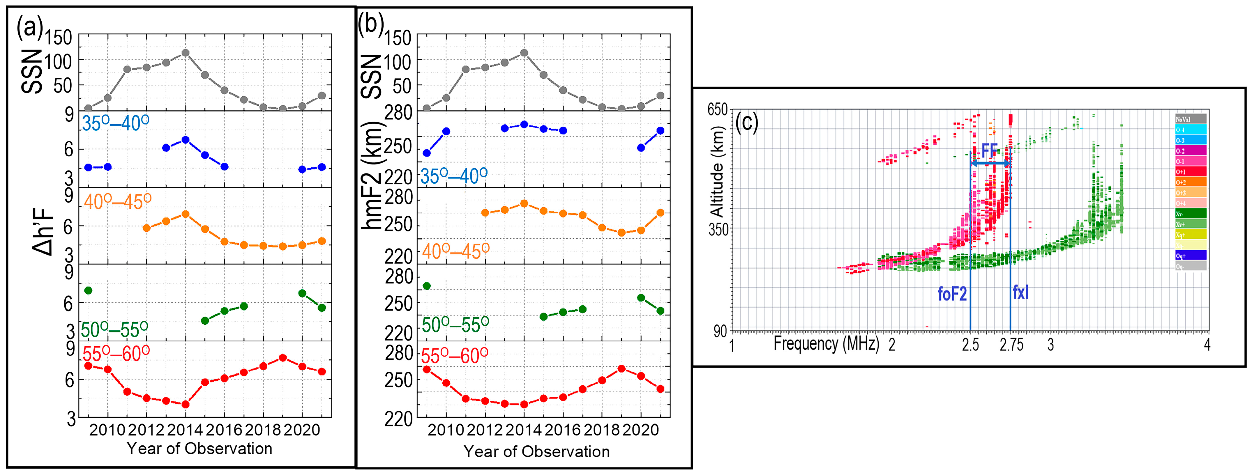
Threshold Estimation for Δh′F and hmF2

To define threshold values a and b for Δh′F and hmF2, we adopted a Gaussian distribution. According to the empirical rule for a normal (Gaussian) distribution, approximately 68%, 95%, and 99.7% of the data lie within 1σ, 2σ, and 3σ from the mean, respectively. We selected 2σ as the threshold to capture significant deviations that are likely associated with SF activity. Figure 3 illustrates a schematic example used to determine the threshold values for Δh′F and hmF2.
To derive the standard deviation σ from the fitted Gaussian distribution, we used the relation
σ = F W H M 2.35
where FWHM is the full width at half maximum of the distribution. Using this, the thresholds a and b for Δh′F and hmF2, respectively, were computed as:
a , b = P e a k ( y ) 2 σ ( y )
where y represents the count of occurrences from the Gaussian distribution curve. This method was applied to each of the four latitude regions, allowing us to capture regional and temporal variations in the thresholds.
Figure 4a,b illustrates the yearly computed a and b values for each latitude region alongside the corresponding yearly average SSN, presented in the top panel to explore solar cycle influences. The results reveal a clear solar activity dependence of both a and b. In the lower midlatitude region (35°–45° N), a and b values increase with rising solar activity, indicating a decreased probability of SF occurrence during solar maxima, as larger thresholds make it harder for Δh′F or hmF2 to exceed them. This observation aligns with previous studies that SF occurrence in this region is inversely proportional to solar activity [4,5]. Conversely, in the higher midlatitude region (≥50° N), a and b tend to decrease during high solar activity periods, implying a higher SF occurrence probability, with the opposite trend expected during solar minimum.

Threshold Estimation for FF

Unlike Δh′F and hmF2, the FF parameter—defined as the difference between fxl and foF2—is calculated for every ionogram regardless of whether FSF is actually present. This complicates the use of traditional statistical methods for threshold estimation, as FF values alone do not reliably indicate FSF occurrence. Instead, to determine a meaningful threshold c, we relied on the visual inspection of ionograms and associated parameters.
Through this manual analysis, we observed that FSF is typically detected only when FF exceeds 0.2 MHz, i.e., fxl − foF2 > 0.2 MHz. This empirical condition was therefore adopted as the operational threshold for c. An example of this behavior is provided in Figure 4c, where FSF is visually confirmed in an ionogram with FF > 0.2 MHz.

3.1.3. Statistics for Common Observation

Since the primary objective of this study was to evaluate the accuracy of the proposed SF detection algorithm, we derived a, b, and c for each latitude region using a single representative station, and then validated these thresholds against other stations within the same latitude region. The selection and validation scheme is as follows:
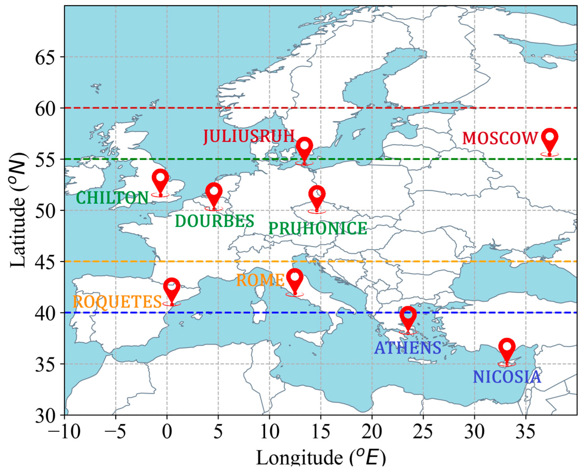
  • 35°–40° N: Thresholds were derived from Nicosia and validated over Athens and Nicosia.
  • 40°–45° N: Thresholds were derived from Roquetes and validated over Roquetes and Rome.
  • 50°–55° N: Thresholds were derived from Pruhonice and validated over Pruhonice, Dourbes, and Chilton.
  • 55°–60° N: Thresholds were derived from Moscow and validated over Moscow and Juliusruh.

3.2. Manual SF Detection

Manual identification of SF (SFM) events in ionograms presents a significant challenge due to the absence of universally accepted or standardized criteria that can distinguish SF-affected ionograms from those recorded during quiet conditions. Although no rigid framework exists, several prior studies have offered empirical guidelines and observational clues that assist current researchers in recognizing these events with reasonable confidence.
In our study, we categorized SF events into two main types: RSF and FSF. For RSF detection, we drew upon insights reported by Hajkowicz (2007) [12], who identified distinct latitudinal variations in RSF occurrence. According to his findings, RSF is prevalent between latitudes 52° and 48° S and continues into the midlatitude zone of 44°–48° S, characterized by a peak spread range (Sr) of approximately 50 km. A notable minimum in RSF occurrence was observed around 42°–43° S, where Sr typically falls around 10 km. In contrast, the identification of FSF events remains more ambiguous, as there are currently no well-established or standardized procedures described in the literature for their identification. Consequently, our FSF identification approach was developed independently, based on frequency spread characteristics observed in the ionograms.
For manual analysis, we restricted our focus to post-sunset ionograms—targeting nighttime during specific time intervals outlined in Table 2. To determine the duration and characteristics of SF events over the 2009–2021 period, we conducted a comprehensive visual inspection of each ionogram, meticulously searching for trace spreading. In the case of RSF events, we adopted a criterion based on the vertical spread along the altitude axis. If the F region trace exhibited a spreading range between 10 km and 50 km, we classified it as RSF. It is important to note that throughout the visual inspection of millions of ionograms over a 13-year period across midlatitude regions, we did not encounter any RSF cases where the vertical spread exceeded 50 km. FSF events were identified based on horizontal spreading along the frequency axis. Specifically, ionograms exhibiting a frequency spread in the range of 0.2 to 1 MHz were classified as FSF events (as illustrated in Figure 4c). Due to the lack of predefined detection methods in the literature for FSF, this frequency range was selected based on empirical observations during manual analysis. To ensure reliability in event classification, we imposed a temporal consistency condition: only those SF events that persisted across three or more consecutive ionograms—each separated by 5-min intervals, corresponding to a minimum duration of 15 min—were considered in this study [6]. Additionally, any ionograms in which the spread Es layer blanketed or obscured the F region trace were excluded from the analysis to avoid misclassification.
To assess the performance of the detection algorithm, we compared SFP with SFM. The accuracy of the prediction was quantified using the following metric, referred to as CommonObs, which represents the percentage of overlap between manual and automated SF detections:
C o m m o n O b s ( % ) = S F M S F P S F P × 100

4. Result and Discussion

In this section, the primary objective is to perform a comprehensive comparative analysis between SFM and the SFP for nine European Digisonde stations. This comparison aims to assess the reliability of auto–scaled SF detection parameters with respect to latitude from 35° N to 60° N.
For each station within these zones, we applied the threshold values a, b, and c—derived for the respective latitude sectors—to compute the SFP. These were then compared for each year with the corresponding SFM. The accuracy of the automated detection method was evaluated using the CommonObs metric.
Subsequently, we conducted an analysis of the relative CommonObs values across all available years for each latitude grid to investigate the effectiveness of the automated SF detection varied with latitude, offering insights into whether detection accuracy is influenced by regional ionospheric dynamics.

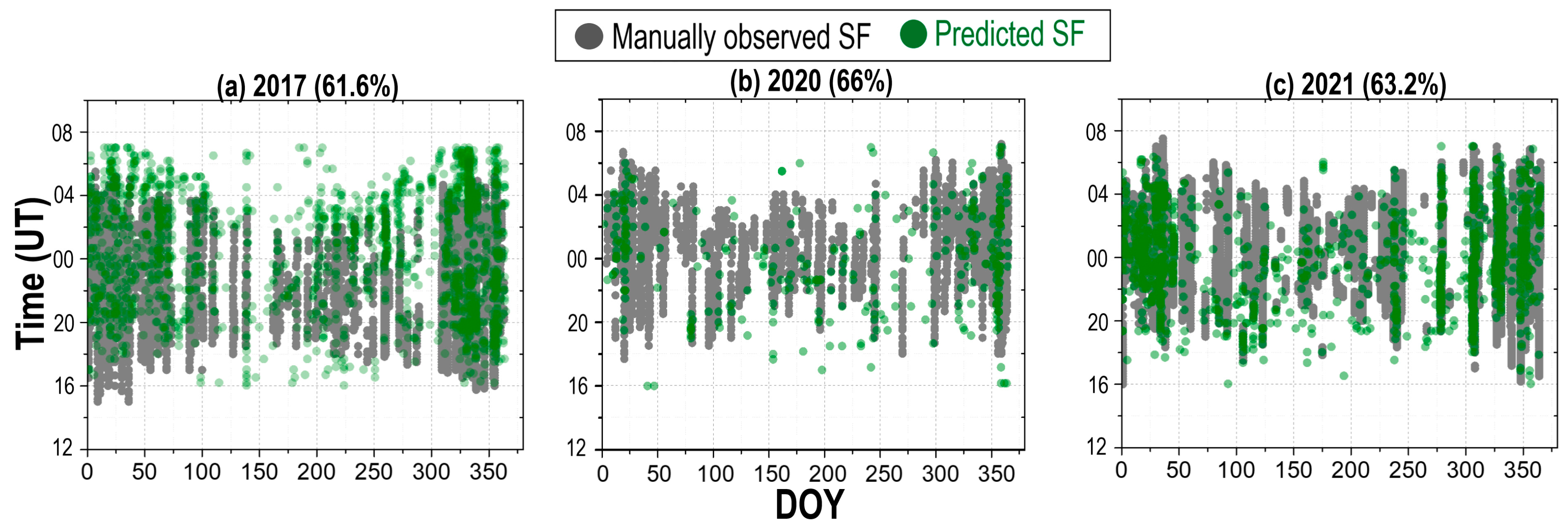
4.1. 55°–60° N Latitude

As previously discussed in Section 3, the 55–60° N latitude region includes two Digisonde stations: Moscow and Juliusruh. The manual detection of SF events at these stations has been well documented in earlier studies by Paul et al. (2022, 2023) [5,6], who reported a direct correlation between SF occurrence and solar activity. Alongside Deminov et al. (2025) [30], they also highlighted a clear influence of the solar terminator, with seasonal maxima in SF activity occurring during winter months—an important consideration for both detection and forecasting efforts.
In the present study, we present a 13-year comparative analysis of SF activity over Moscow, covering the period from 2009 to 2021, as illustrated in Figure 5a–m. SF events were manually identified within the time window of 14:00 UT to 10:00 UT (next day), consistent with the expected nighttime ionospheric conditions at this latitude. The same temporal range was used to extract auto-scaled data from GIRO. In each subplot of Figure 4, the x-axis represents the day of the year (DOY), and the y-axis corresponds to the hour of the day. Grey markers indicate SFM, while red markers denote SFP. The CommonObs value, quantifying the agreement between SFM and SFP, is provided for each year.
From the figure, a consistent pattern emerges: across all years, SFP tends to overestimate SF occurrence compared to SFM, particularly during the equinoxes and summer months, and most prominently during high solar activity years (2011–2015). Notably, the CommonObs value exhibits an inverse relationship with solar activity—as solar activity increases, CommonObs decreases, and vice versa. While lower solar activity years generally show better alignment between SFM and SFP, high activity years, especially 2012–2015, display poor correspondence.
Comparative SF observations for 2017, 2020, and 2021 over Juliusruh are presented in Figure 6a–c. Although all three years are characterized by low solar activity, notable variations in CommonObs values are still evident. Similar to the trends observed in Moscow, SFP overestimates SFM, especially during equinox and summer, even under relatively quiet solar conditions. Furthermore, the accuracy of SFP improves as solar activity decreases, mirroring the findings from Moscow. This indicates that while the algorithm performs reasonably well during solar minimum years, its reliability is reduced during more active periods, possibly due to increased ionospheric variability.

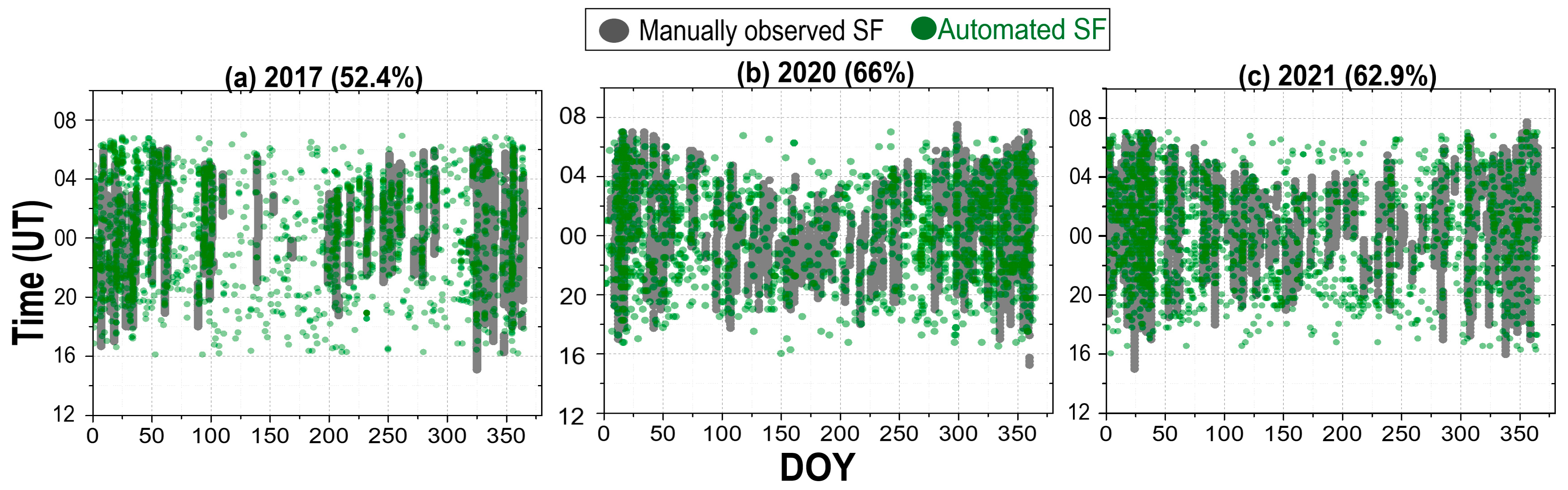
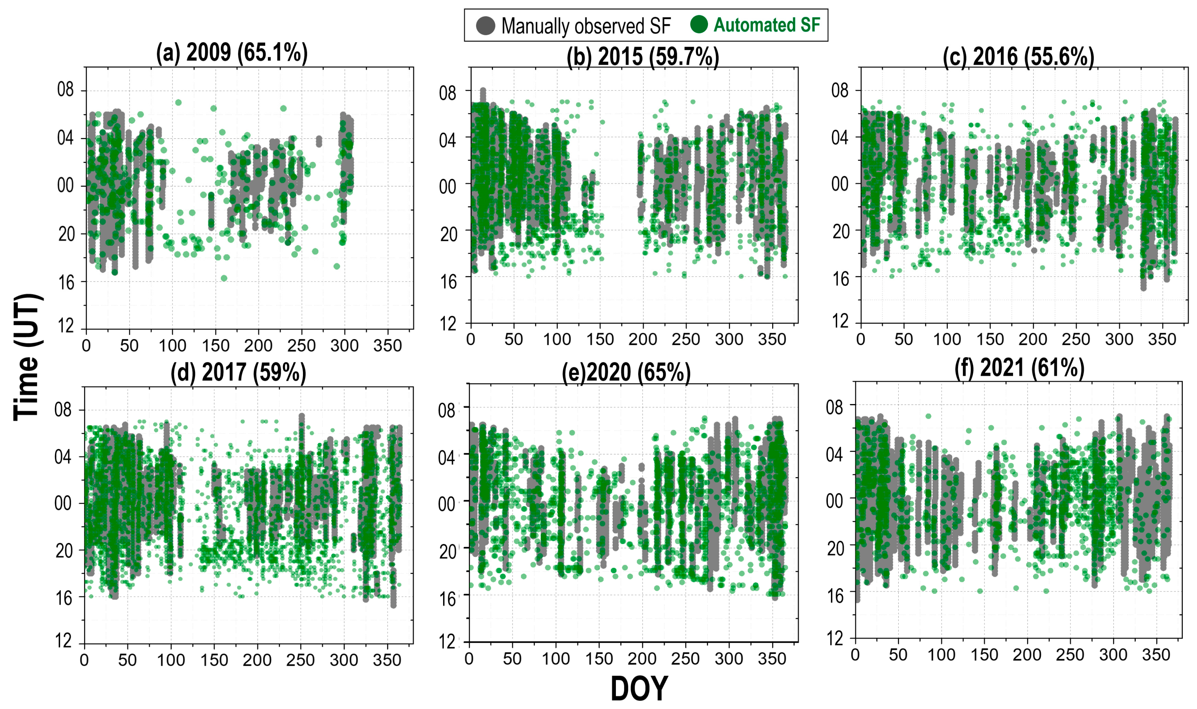
4.2. 50°–55° N Latitude

Three stations—Chilton, Dourbes, and Pruhonice—located within the 50°–55° N latitude region, have been the focus of long-term studies on SF activity, with manual observations documented extensively by Paul et al. (2018; 2023) [3,6]. These studies indicate a possible dependence on solar activity, alongside a clearly observed solar terminator influence, with peak SF occurrence during winter months over all three stations [6].
For Chilton, manual SF observations for the years 2017, 2020, and 2021 are presented in Figure 7a–c. The comparison reveals contradicting patterns across different years: in 2017, SFP overestimated SFM, particularly during the post-midnight to dawn hours, whereas in 2020 and 2021, SFP underestimated SFM, suggesting variability in auto–scaling performance across different solar conditions. Notably, 2020 data showed a significantly lower number of auto–scaled dataset, which may have influenced the comparison results. However, during winter months, typically the period of maximum SF activity, a stronger association between SFP and SFM was observed, while summer months—especially during moderate solar activity—showed lower agreement.
Similar trends were observed at Dourbes, as shown in Figure 8a–c, covering the same years. In 2017, the algorithm overpredicted SF events relative to manual detection, with the largest discrepancies during early evening hours (~16:00 to 20:00 UT) in summer. In contrast, the agreement between SFP and SFM improved in 2020 due to lower solar activity but was again reduced in 2021, coinciding with a shift from low to moderate solar activity levels.
The most extensive dataset in this latitude region comes from Pruhonice, for which six years of comparative data (2009, 2015–2017, 2020–2021) are shown in Figure 9a–f. In 2009 and 2020, we observed notably less records in the auto–scaled data, which may have limited the reliability of SFP assessment for those years. Still, a clear pattern emerged: CommonObs values tend to decline with increasing solar activity, even during moderate solar activity years, like 2015 and 2017. Despite this, winter SF maxima consistently show stronger agreement between manual and automated detection, regardless of solar conditions, reaffirming the role of seasonal dynamics in algorithm performance. During the equinoxes and summer months, particularly in post-sunset hours, the algorithm overestimated SF occurrence.

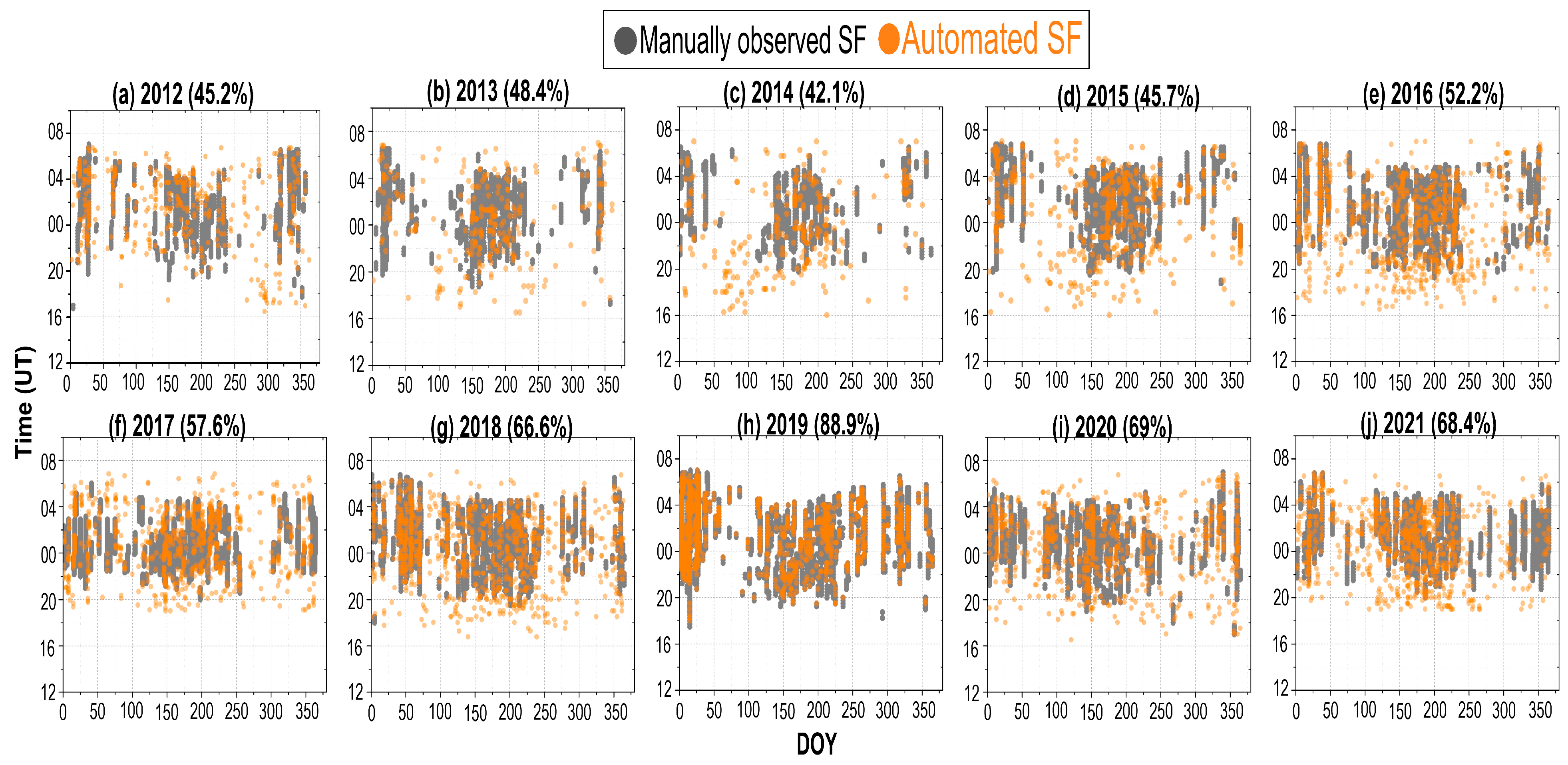
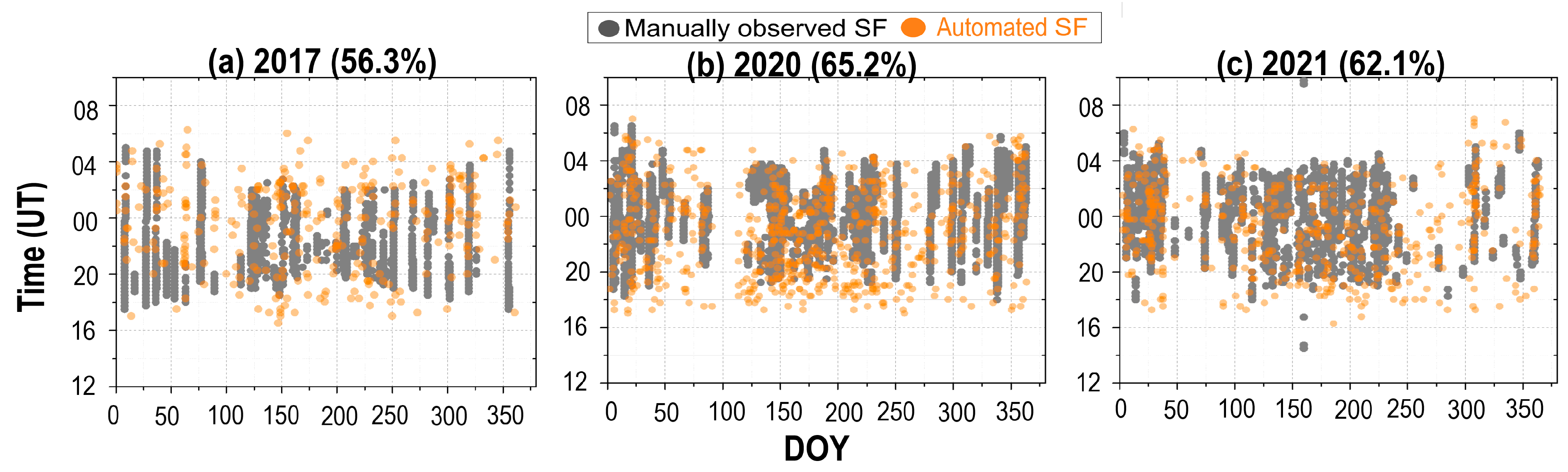
4.3. 45°–40° N Latitude

The 40°–45° N latitude region, encompassing Roquetes and Rome, has received limited attention in terms of long-term climatological studies on SF occurrence. Paul et al. (2023) [6] reported that stations within this latitude region tend to exhibit lower SF occurrence compared to those located above 50° N and that SF maxima in this region are more commonly observed during summer months.
In this study, we present a comparative analysis over Roquetes from 2012 to 2021, covering nearly a full solar cycle. Figure 10a–j displays the temporal and diurnal distribution of both SFM (grey dots) and SFP events (orange dots). From the figures corresponding to higher solar activity (2012–2016, panels a–e), a moderate agreement between SFM and SFP is observed, with notable overestimation of SFP, particularly during post-sunset hours (~16:00 to 19:00 UT). However, as solar activity declined, the association between SFM and SFP improved substantially, as seen in Figure 10f–j. During 2019, the agreement peaked at 89%, marking a significant improvement in detection accuracy (Figure 10h). Across 2018–2020, the data show a clear trend of increasing CommonObs values, suggesting that the auto-scaled detection method performs more reliably during lower solar activity. However, some degree of overestimation during the equinoctial and post-sunset summer periods still persisted.
For Rome, only three years of data (2017, 2020, and 2021) were available for analysis, as shown in Figure 11a–c. The 2017 dataset, presented in Figure 10a, was characterized by significant auto-scaling error, limiting the reliability of SFP results. Nonetheless, an overestimation of SFP during post-sunset summer hours (~16:00 to 19:00UT) was still evident. In 2020 and 2021, Rome exhibited trends similar to Roquetes, with a notable improvement in agreement between SFM and SFP as solar activity declined. While 2020 still showed some SFP overestimation during post-sunset summer periods, the overall association between manual and automated detection was considerably better compared to 2017.

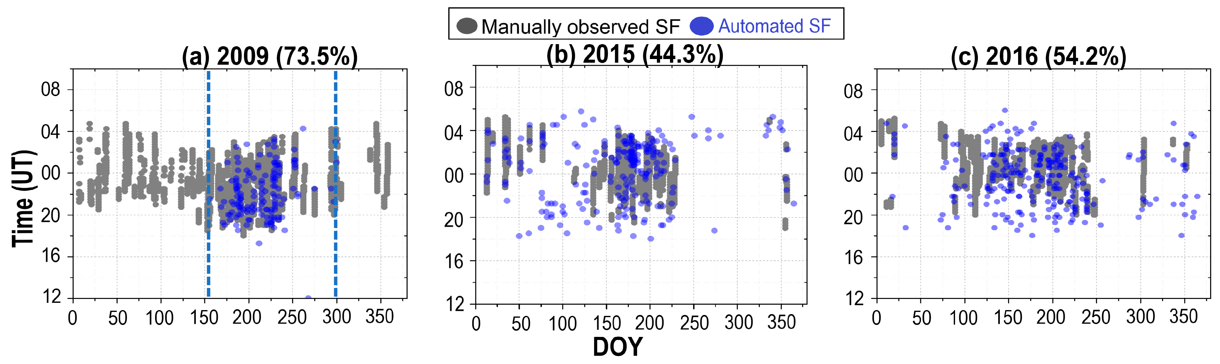
4.4. 35°–40° N Latitude

The final latitude sector examined in this study is 35°–40° N, which includes Nicosia and Athens. These two stations exhibit SF occurrence characteristics similar to those of Roquetes and Rome, as reported by Paul et al. (2018, 2023) [3,6]. Long-term climatological studies over Nicosia by Paul et al. (2019, 2022) [4,5] revealed that SF occurrence in this region decreases during high solar activity periods and increases during the solar minimum. However, during moderate solar activity, no significant correlation between SF occurrence and solar conditions was observed. Additionally, these studies indicated that SF activity peaks during summer, regardless of solar activity.
The comparison between SFM and SFP over Athens is presented in Figure 12a–c for 2009, 2015, and 2016. It is important to note that while full-year ionogram data were available for 2009, GIRO auto–scaled data were only available from June to October, as shown by the blue dotted lines in Figure 12a. Despite relative agreement between SFM and SFP in these years, the seasonal occurrence pattern aligned well, especially in 2015 and 2016. As seen in Figure 12c, SFP overestimated SF activity during post–sunset hours (~18:00 to 20:00 UT) of summer 2016, whereas in 2015 (Figure 12b), the overestimation occurred predominantly during post-sunset hours of the vernal equinox.
For Nicosia, a more extended dataset was available, as shown in Figure 13a–h, covering 2009–2010, 2013–2016, and 2020–2021. During the low solar activity years of 2009 and 2010, the association between SFM and SFP was high, with strong seasonal agreement (Figure 13a,b). As solar activity increased, a significantly lower agreement was noted, particularly in 2013–2015, when SFP overestimated SF occurrence, mainly during winter and autumnal equinox (Figure 13c–e). By 2016, as solar activity declined, the agreement between SFM and SFP improved, though an overestimation was still noted in January–February (Figure 13f). An underestimation of SF activity by SFP was observed during November–December, suggesting a decline in automated detection performance. Due to technical issues, 2020–2021 data for Nicosia were incomplete, limiting the reliability of the analysis for this period (Figure 13g,h). However, even with sparse data, the trend of improved SFM–SFP agreement during lower solar activity remained.
From the above observations, a clear pattern emerges regarding the association between SFM and SFP across the European midlatitudes, specifically within the 35°–60° N latitude range. To represent this association, we calculated the yearly average values of the CommonObs metric—by aggregating results from all stations within each latitude sector. These averaged values are presented collectively in Figure 14b–e, while Figure 14a provides the yearly average SSN. By comparing the SSN trends with CommonObs values across different latitudinal sectors, we can evaluate the impact of solar activity on the accuracy of automated SF detection.
The estimated average CommonObs values for the 55°–60° N latitude sector, shown in Figure 14b, exhibited a clear inverse trend with solar activity. During the low solar activity period of 2009–2010, a high agreement between SFM and SFP was observed, consistent with the results in Figure 5a–m and Figure 6a–c. As solar activity increased, the CommonObs values steadily declined, reaching a minimum around the 2014–2015 solar maximum, before rising again from 2016 onward and peaking in 2018–2019. This trend indicates that the reliability of the automated detection algorithm improves during the solar minimum and degrades during the solar maximum. Notably, an overestimation of SFP relative to SFM was evident during equinox and summer periods, likely due to the dominance of FSF in this region, where large-scale TIDs (LSTIDs) are a key SF driver [5,6]. However, the literature also indicates that this latitude range is influenced by polar dynamics and the midlatitude ionospheric trough (MIT) [30,31], suggesting that TID activity cannot fully account for SF formation. In many cases, TID–associated ionogram signatures are not always scalable or detectable through auto–scaling methods, increasing the risk of undetected or misinterpreted TID activity. Moreover, SF generation requires a combination of favorable ionospheric conditions beyond just TID activity. Therefore, we believe that during equinox and summer, especially in high solar activity years, TIDs can drive F region uplifts but not to the extent necessary for SF formation, leading to false SF event detection by the algorithm which thereby overestimates SFP compared to actual SFM.
The estimated average CommonObs values for the 50°–55° N latitude sector, as shown in Figure 14c, revealed higher agreement between SFM and SFP during low solar activity compared to high solar activity, although a clear solar cycle dependence cannot be conclusively established due to limited data. A key observation in this sector is the frequent overestimation of SFP, particularly during post-sunset hours in equinoctial and summer months, notably over Dourbes and Pruhonice, as depicted in Figure 8a–c and Figure 9a–f. In contrast, Chilton exhibited overestimation predominantly during post-midnight hours (~04:00 to 07:00 UT), as seen in Figure 7a–c. This behavior can be attributed to the susceptibility to medium-scale TIDs (MSTIDs), which according to Paul et al. (2023) [6] and Otsuka et al. (2013) [32], commonly propagate from the northwest to southeast across Europe. MSTIDs typically generate oblique traces in ionograms [33], which may resemble SF-associated features and cause F layer uplifts without necessarily triggering SF events. These uplifts manifested as higher hmF2 and h′F values, which the auto-scaling algorithm might misinterpret as SF. However, when MSTID-induced oblique traces merge with the main O trace, it becomes challenging for the algorithm to accurately detect true frequency spread, potentially compromising the reliability of FF as an SF indicator. Additionally, as previously discussed [6], actual SF occurrence is relatively lower in this latitude sector during the summer and equinox, despite MSTID activity. This implies that although MSTIDs can appear as SF activity in ionograms, the lack of favorable background conditions prevents SF development, thereby contributing to errors in automated SF detection.
Figure 14d shows the estimated average CommonObs values between 40° and 45° N, revealing an inverse relationship with solar activity over the ten-year period. A minimum in CommonObs was observed around 2014, coinciding with the solar maximum in Solar Cycle 24, while the highest association between SFP and SFM occurred around 2019. Despite this trend, Figure 10a–j, Figure 11a–c and Figure 14a–e indicate that stations below 50° N consistently exhibit stronger SFP–SFM association, regardless of solar activity.
Figure 14e presents the estimated average CommonObs values for the 35°–40° N latitude range, based on eight years of data, revealing a clear inverse relationship with solar activity. A strong SFP–SFM association was observed in 2009–2010, which diminished as solar activity increased, reaching a minimum in 2014, and then rising again with decreasing solar activity. Similar to the trends seen in the 40°–45° N sector, this region also shows consistent inverse solar dependence.
In the low midlatitude ionosphere, while clear TID signatures are not always evident in ionograms, other features have been associated with wave activity [3,4,34]. Two such notable ionogram features are satellite traces (STs) and multiple reflected echoes (MREs), first described by McNicol et al. (1956) [35] and later examined in detail by Paul et al. (2018, 2019, 2021) [3,4,33]. STs are typically observed in ionograms during moderate to high levels of solar activity, particularly during the post-sunset period. As reported by Paul et al. (2021) [33], STs tend to appear at the trailing edge of the F layer trace and have been extensively investigated in low equatorial studies. They have been associated with wave-like ionospheric perturbations. Similarly, MREs are also indicative of wave activity and appear on ionograms over specific segments not confined to any specific layer. According to Paul et al. (2021) [33], MREs are especially prominent during winter months during high solar activity years. STs and MREs pose significant challenges to the accuracy of automated SF detection As they may contribute to an overestimation of SFP, particularly during the post–sunset hours of the equinox and summer months, as demonstrated in Figure 3 (p. 4) of Paul et al. (2021) [33]. Additionally, similar misidentifications can occur during winter, as shown in Figure 4 (p. 5) of the same study. Overall, these ionogram signatures are a key factor in the discrepancies between SFM and SFP over the low midlatitude ionosphere.
An important aspect to highlight in this discussion is that, although the primary focus has been on the overestimation of SFP relative to SFM, evidence from Figure 10, Figure 11, Figure 12 and Figure 13 indicates that underestimation also occurs in certain cases—particularly during summer periods when SF occurrence peaks over the low midlatitude ionosphere. This underestimation is primarily due to the presence of spread Es events [3,4,36], which are common during summer in these regions. Spread Es arises when oblique ionogram traces appear on the Es layer. Although spread Es is recognized in the literature as a driver of SF formation through E–F layer electrodynamic coupling, it poses a challenge for automated detection. Specifically, the auto–scaling algorithm struggles to detect the F trace when it is obscured by the spread Es layer—a phenomenon known as “blanketing” the F trace. As a result, the algorithm fails to detect SF, leading to an underestimation of actual SF events despite their presence in the ionogram.

5. Conclusions

In this study, we evaluated the performance and reliability of an automated SF detection algorithm by integrating SF-related and ionospheric parameters derived from ARTIST of SAO Explorer auto-scaled data and comparing the algorithm outputs with manually identified SF events across nine European midlatitude ionospheric stations. These stations were grouped into four latitude sectors to examine potential latitudinal effects on the algorithm’s performance. To explore the influence of solar activity, the algorithm was applied to an extended dataset spanning from 2009 to 2021. The analysis revealed a clear inverse relationship between solar activity and the agreement between automated and actual SF occurrence—a stronger association was observed during periods of low solar activity, regardless of latitude. Additionally, the CommonObs metric exhibited notable latitudinal variation in the agreement between SFP and SFM. The primary conclusions from this investigation are summarized as follows:
i.
In the 55°–60° N latitude sector, the association between automated SFP and SFM events ranged from a maximum of 71% during the solar minimum to a minimum of 47% during the solar maximum. The algorithm frequently overestimated SFP occurrences during periods of high solar activity, which is primarily attributed to LSTID activity that can mislead the detection algorithm.
ii.
The association between SFP and SFM in the 50°–55° N latitude sector reached a maximum of 66% during the solar minimum and a minimum of 56% during the solar maximum. Overestimation by SFP was predominantly observed during post-sunset hours during the equinox and summer under high solar activity. This overestimation is likely due to the presence of oblique traces or MSTIDs, which can interfere with accurate SF detection by resembling spread signatures in ionograms.
iii.
In the 40°–45° N latitude sector, the association between SFM and SFP reached a maximum of 89% during the solar minimum and dropped to a minimum of 42% during the solar maximum. SFP overestimated SFM, particularly during post-sunset hours in the equinoctial and summer months under high solar activity, likely due to the presence of STs and MREs, which can mimic SF signatures and confuse the auto-scaling algorithm. Conversely, during summer periods when SF occurrence is generally high in this region, SFP may have underestimated SFM. This underestimation is likely attributed to the presence of spread Es, which can blanket the F layer trace in ionograms, leading to scaling errors and the failure of the algorithm to detect actual SF events.
iv.
The SFM and SFP association in the 35°–40° N latitude sector varied from a maximum of 69% during the solar minimum to a minimum of 30% during the solar maximum. Overestimation by SFP was mostly noted during winter and high solar activity, which may have resulted from the STs and MREs that interfere with accurate SF detection. Additionally, during summer periods—when SF events are more frequent in this sector—SFP may have underestimated SFM, likely due to spread Es. These irregular Es layer structures can blanket the F trace in ionograms, preventing the auto-scaling algorithm from correctly identifying SF events and resulting in missed detections.

Author Contributions

Conceptualization, K.S.P. and H.H.; methodology, K.S.P.; software, T.B.; validation, K.S.P., H.H. and T.B.; formal analysis, K.S.P. and T.B.; investigation, K.S.P.; resources, H.H.; data curation, K.S.P., H.H. and T.B.; writing—original draft preparation, K.S.P.; writing—review and editing, K.S.P., T.B. and H.H.; visualization, K.S.P. and T.B.; supervision, H.H. and K.S.P.; project administration, K.S.P.; funding acquisition, K.S.P. All authors have read and agreed to the published version of the manuscript.

Funding

Funding for this research was provided by the project “Towards A Global Model for Spread F”—TAGMOS-F (Ref No: EXCELLENCE/0524/0526), which is co-funded by the Republic of Cyprus and the European Regional Development Fund (ERDF) through the ‘EXCELLENCE HUBS’ Program, in the frame of the Operational Program “ΘAλΕΙA” 2021–2027.

Institutional Review Board Statement

Not applicable.

Informed Consent Statement

Not applicable.

Data Availability Statement

In the present analysis, all the data used are freely available to the public domain. The ionograms used for manual SF detection are available at (https://giro.uml.edu/ionoweb/ accessed on 4 March 2025). The automated SF detection data were downloaded from the FastChar database hosted on the DIDBase platform (https://giro.uml.edu/didbase/scaled.php accessed on 7 March 2025). And finally, the yearly average sunspot number data are available at https://www.sidc.be/SILSO/datafiles (accessed on 11 March 2025).

Acknowledgments

We are thankful to the Digital Ionogram DataBase (DIDBase) of the Global Ionospheric Radio Observatory (GIRO) portal (https://giro.uml.edu/didbase/acknowledgements.html accessed on 4 March 2025) for the ionograms and FastChar website (https://giro.uml.edu/didbase/scaled.php accessed on 7 March 2025). Finally, we are grateful to the project “Towards A Global Model for Spread F”—TAGMOS-F (Ref No: EXCELLENCE/0524/0526), which is co-funded by the Republic of Cyprus and the European Regional Development Fund (ERDF) through the ‘EXCELLENCE HUBS’ Program, in the frame of the Operational Program “ΘAλΕΙA” 2021–2027.

Conflicts of Interest

Author Trisani Biswas was employed by the company GeoImaging Ltd. The remaining authors declare that the research was conducted in the absence of any commercial or financial relationships that could be construed as a potential conflict of interest.

References

  1. Bowman, G.G. Frontal and non-frontal characteristics of mid-latitude spread-F structures. Indian J. Radio Space Phys. 1990, 19, 62–68. [Google Scholar]
  2. Bowman, G.G. The influence of 10.7-cm solar-flux variations on midlatitude daytime ionospheric disturbance conditions. J. Geophys. Res. 1996, 101, 10849–10854. [Google Scholar] [CrossRef]
  3. Paul, K.S.; Haralambous, H.; Oikonomou, C.; Paul, A.; Belehaki, A.; Ioanna, T.; Kouba, D.; Buresova, D. Multi-station investigation of spread F over Europe during low to high solar activity. J. Sp. Weather Sp. Clim. 2018, 8, A27. [Google Scholar] [CrossRef]
  4. Paul, K.S.; Haralambous, H.; Oikonomou, C.; Paul, A. Long-term aspects of nighttime spread F over a low mid-latitude European station. Adv. Space Res. 2019, 64, 1199–1216. [Google Scholar] [CrossRef]
  5. Paul, K.S.; Haralambous, H.; Singh, A.K.; Gulyaeva, T.L.; Panchenko, V.A. Mid-latitude Spread F long-term occurrence characteristics as a function of latitude over Europe. Adv. Space Res. 2022, 70, 710–722. [Google Scholar] [CrossRef]
  6. Paul, K.S.; Haralambous, H.; Oikonomou, C.; Singh, A.K.; Gulyaeva, T.L.; Panchenko, V.A.; Altadill, D.; Buresova, D.; Mielich, J.; Verhulst, T. A mid-latitude spread F over an extended European area. J. Atmos. Sol.-Terr. Phys. 2023, 248, 106093. [Google Scholar] [CrossRef]
  7. Vasylyev, D.; Béniguel, Y.; Volker, W.; Kriegel, M.; Berdermann, J. Modeling of ionospheric scintillation. J. Sp. Weather Sp. Clim. 2022, 12, 22. [Google Scholar] [CrossRef]
  8. Huang, W.Q.; Xiao, Z.; Xiao, S.G.; Zhang, D.H.; Hao, Y.Q.; Suo, Y.C. Case study of apparent longitudinal differences of spread F occurrence for two mid-latitude stations. Radio Sc. 2011, 46. [Google Scholar] [CrossRef]
  9. Bhaneja, P.; Earle, G.D.; Bishop, R.L.; Bullett, T.W.; Mabie, J.; Redmon, R. A statistical study of mid-latitude spread F at Wallops Island, Virginia. J. Geophys. Res. 2009, 114, A04301. [Google Scholar] [CrossRef]
  10. Miller, C.A.; Swartz, W.E.; Kelley, M.C.; Mendillo, M.; Nottingham, D.; Scali, J.; Reinisch, B. Electrodynamics of midlatitude spread F: 1. Observations of unstable, gravity wave-induced ionospheric electric fields at tropical latitudes. J. Geophys. Res. Sp. Phys. 1997, 102, 11521–11532. [Google Scholar] [CrossRef]
  11. Fejer, B.G.; Kelley, M.C. Ionospheric irregularities. Rev. Geophys. 1980, 18, 401–454. [Google Scholar] [CrossRef]
  12. Hajkowicz, L.A. June. Morphology of quantified ionospheric range spread-F over a wide range of midlatitudes in the Australian longitudinal sector. Ann. Geophys. 2007, 25, 1125–1130. [Google Scholar] [CrossRef]
  13. Dyson, P.L.; Newton, G.P.; Brace, L.H. In situ measurements of neutral and electron density wave structure from the Explorer 32 satellite. J. Geophys. Res. 1970, 75, 3200–3210. [Google Scholar] [CrossRef]
  14. Hines, C.O. The upper atmosphere in motion. Q. J. Roy. Meteorol. Soc. 1963, 89, 1–42. [Google Scholar] [CrossRef]
  15. Bowman, G.G. A relationship between ‘‘spread-F” and the height of the F2 ionospheric layer. Aust. J. Phys. 1960, 13, 69–72. [Google Scholar] [CrossRef]
  16. Singleton, D.G. The morphology of spread-F occurrence over half a sunspot cycle. J. Geophys. Res. 1968, 73, 295–308. [Google Scholar] [CrossRef]
  17. Igarashi, K.; Kato, H. Solar cycle variations and latitudinal dependence on the midlatitude spread F occurrence around Japan. In Proceedings of the XXIV General Assembly, Kyoto, Japan, 25 August–2 September 1993. [Google Scholar]
  18. Bowman, G.G. A comparison of nighttime TID characteristics between equatorial ionospheric-anomaly crest and midlatitude regions, related to spread F occurrence. J. Geophys Res. 2001, 106, 1761–1769. [Google Scholar] [CrossRef]
  19. Shimazaki, T. A statistical study of occurrence probability of spread F at high latitudes. J. Geophys. Res. 1962, 67, 4617–4634. [Google Scholar] [CrossRef]
  20. Singleton, D.G. Spread-F and the parameters of the F-layer of the ionosphere—II: Spread-F and F-layer height. J. Atmos. Terr. Phys. 1962, 24, 885–898. [Google Scholar] [CrossRef]
  21. Khmyrov, G.M.; Galkin, I.A.; Kozlov, A.V.; Reinisch, B.W.; McElroy, J.; Dozois, C. Exploring digisonde ionogram data with SAO-X and DIDBase. In AIP Conference Proceedings; American Institute of Physics: College Park, MD, USA, 2008; Volume 974, pp. 175–185. [Google Scholar]
  22. Reinisch, B.W.; Galkin, I.A. Global ionospheric radio observatory (GIRO). Earth Planets Sp. 2011, 63, 377–381. [Google Scholar] [CrossRef]
  23. Bilitza, D.; Pezzopane, M.; Truhlik, V.; Altadill, D.; Reinisch, B.W.; Pignalberi, A. The International Reference Ionosphere model: A review and description of an ionospheric benchmark. Rev. Geophys. 2022, 60, e2022RG000792. [Google Scholar] [CrossRef]
  24. Paul, K.S.; Haralambous, H. Assessment of the Midlatitude SF Detection. In Proceedings of the Remote Sensing and Geoinformation of Environment, Paphos, Cyprus, 17–19 March 2025. [Google Scholar]
  25. Galkin, I.A.; Reinisch, B.W. The new ARTIST 5 for all digisondes. Proc. Ionosonde Netw. Advis. Group Bull. 2008, 69, 1–8. [Google Scholar]
  26. Bamford, R.A.; Stamper, R.; Cander, L.R. A comparison between the hourly autoscaled and manually scaled characteristics from the Chilton ionosonde from 1996 to 2004. Radio Sci. 2008, 43, 1–11. [Google Scholar] [CrossRef]
  27. Hofmann-Wellenhof, B.; Lichtenegger, H.; Wasle, E. GNSS–Global Navigation Satellite Systems: GPS, GLONASS, Galileo, and More; Springer Wien: NewYork, NY, USA, 2007. [Google Scholar]
  28. Scotto, C.; Ippolito, A.; Sabbagh, D. A method for automatic detection of equatorial spread-F in Ionograms. Adv. Space Res. 2019, 63, 337–342. [Google Scholar] [CrossRef]
  29. Rao, T.V.; Sridhar, M.; Ratnam, D.V. Auto-detection of sporadic E and spread F events from the digital ionograms. Adv. Space Res. 2022, 70, 1142–1152. [Google Scholar] [CrossRef]
  30. Deminov, M.G.; Nepomnyashchaya, E.V.; Sitnov, Y.S. Regularities of the midlatitude spread F occurrence probability during sunrises and sunsets. Geomag. Aeron. 2005, 45, 458–465. [Google Scholar]
  31. Liu, Y.; Xiong, C.; Wan, X.; Lai, Y.; Wang, Y.; Yu, X.; Ou, M. Instability mechanisms for the F-region plasma irregularities inside the midlatitude ionospheric trough: Swarm observations. Sp. Weather 2021, 19, e2021SW002785. [Google Scholar] [CrossRef]
  32. Otsuka, Y.; Suzuki, K.; Nakagawa, S.; Nishioka, M.; Shiokawa, K.; Tsugawa, A. GPS observations of medium-scale travelling ionospheric disturbances over Europe. Ann. Geophys. 2013, 31, 163–172. [Google Scholar] [CrossRef]
  33. Paul, K.S.; Haralambous, H. Investigation for Possible Association of the Topside and Bottomside Ionospheric Irregularities over the Midlatitude Ionosphere. Appl. Sci. 2025, 15, 506. [Google Scholar] [CrossRef]
  34. Paul, K.S.; Haralambous, H.; Oikonomou, C.; Paul, A. Investigation of Satellite Trace (ST) and Multi-reflected Echo (MRE) ionogram signatures and its possible correlation to nighttime spread F development from Cyprus over the solar mini-max (2009–2016). Adv. Space Res. 2021, 67, 1958–1967. [Google Scholar] [CrossRef]
  35. McNicol, R.W.E.; Webster, H.C.; Bowman, G.G. A study of ‘‘Spread-F‘‘ ionospheric echoes at night at Brisbane. I. Range spreading (Experimental). Aust. J. Phys. 1956, 9, 247–271. [Google Scholar] [CrossRef]
  36. Haldoupis, C.; Kelley, M.C.; Hussey, G.C.; Shalimov, S. Role of unstable sporadic-E layers in the generation of mid-latitude spread F. J. Geophys. Res. 2003, 108. [Google Scholar] [CrossRef]
Figure 1. (a,b) Cases recorded over Nicosia in 2016. (a) Auto–scaled SF detection but no SF in manual observation; (b) SF detected both in auto-scaled and manually.
Atmosphere 16 00642 g001
Figure 2. The geographic locations of the Digisondes over Europe were used for the present study. The stations represented by blue lie between 35°–40° N latitude; orange between 35°–40° N; green between 50°–55° N and red between 55°–60° N latitude.
Atmosphere 16 00642 g002
Figure 3. A schematic Gaussian distribution function representation is used to calculate the threshold values of hmF2 and Δh’F. The present example represents the threshold value calculation over Moscow in 2009. The x-axis denotes the parameter (e.g., hmF2 in km), and the y-axis is the counts used for the histogram study.
Atmosphere 16 00642 g003
Figure 4. (ac) The yearly variation of (a) Δh’F and (b) hmF2 threshold values with solar activity over the four latitude region. The 35°–40° N region is represented by blue; 40°–45° N is orange; 50°–55° N is green; and 55°–60° N is red. (c) A schematic example for FF threshold value detection. In this ionogram, FF is 0.25 which clearly indicates the FSF occurrence.
Atmosphere 16 00642 g004
Figure 5. (am) Comparative representation between SFM (grey points) and SFP (red points) over Moscow in (a) 2009, (b) 2010, (c) 2011, (d) 2012, (e) 2013, (f) 2014, (g) 2015, (h) 2016, (i) 2017, (j) 2018, (k) 2019, (l) 2020, and (m) 2021. The CommonObs (%) value for each individual year has been represented at the top of every subsection of the Figure.
Atmosphere 16 00642 g005
Figure 6. (ac). Comparative representation between SFM (grey points) and SFP (red points) over Juliusruh in (a) 2017, (b) 2020, and (c) 2021. The CommonObs (%) value for each individual year has been represented at the top of every subsection of the Figure.
Atmosphere 16 00642 g006
Figure 7. (ac) Comparative representation between SFM (grey points) and SFP (green points) over Chilton in (a) 2017, (b) 2020, and (c) 2021. The CommonObs (%) value for each individual year has been represented at the top of every subsection of the Figure.
Atmosphere 16 00642 g007
Figure 8. (ac) Comparative representation between SFM (grey points) and SFP (green points) over Dourbes in (a) 2017, (b) 2020, and (c) 2021. The CommonObs (%) value for each individual year has been represented at the top of every subsection of the Figure.
Atmosphere 16 00642 g008
Figure 9. (af) Comparative representation between SFM (grey points) and SFP (green points) over Pruhonice in (a) 2009, (b) 2015, (c) 2016, (d) 2017, (e) 2020, and (f) 2021. The CommonObs (%) value for each individual year has been represented at the top of every subsection of the Figure.
Atmosphere 16 00642 g009
Figure 10. (aj) Comparative representation between SFM (grey points) and SFP (orange points) over Roquetes in (a) 2012, (b) 2013, (c) 2014, (d) 2015, (e) 2016, (f) 2017, (g) 2018, (h) 2019, (i) 2020, and (j) 2021. The CommonObs (%) value for each individual year has been represented at the top of every subsection of the Figure.
Atmosphere 16 00642 g010
Figure 11. (ac) Comparative representation between SFM (grey points) and SFP (orange points) over Rome in (a) 2017, (b) 2020, and (c) 2021. The CommonObs (%) value for each individual year at the top of every subsection of the Figure.
Atmosphere 16 00642 g011
Figure 12. (ac) Comparative representation between SFM (grey points) and SFP (blue points) over Athens in (a) 2009 (the blue dotted lines indicate the availability of FastChar data), (b) 2015, and (c) 2016. The CommonObs (%) value for each individual year has been represented at the top of every subsection of the Figure.
Atmosphere 16 00642 g012
Figure 13. (ah) Comparative representation between SFM (grey points) and SFP (blue points) over Nicosia in (a) 2009, (b) 2010, (c) 2013, (d) 2014, (e) 2015, (f) 2016, (g) 2020, and (h) 2021. The CommonObs (%) value for each year has been represented at the top of every subsection of the Figure.
Atmosphere 16 00642 g013
Figure 14. (ae) Overall comparative representation of average CommonObs data and possible association with the SSNs over 35°–60° N latitudes: (a) yearly average SSN data. Average CommonObs data for every year over (b) 55°–60° N, (c) 50°–55° N, (d) 40°–45° N, and (e) 35°–40° N.
Atmosphere 16 00642 g014
Table 1. Geographic coordinates and the years of SF observations for the present study. The color codes represent the latitude regions.
Latitude RangeStationsLatitude (° N)Longitude (°E)Manual SF Detected Years
35°–40°Nicosia35.0333.162009–2010, 2013–2016, 2020–2021
Athens3823.52009, 2015–2016
40°–45°Rome41.812.52017, 2020–2021
Roquetes40.80.52012–2021
50°–55°Pruhonice5014.62009, 2015–2017, 2020–2021
Dourbes50.14.62017, 2020–2021
Chilton51.5–0.62017, 2020–2021
55°–60°Juliusruh54.613.42017, 2020–2021
Moscow55.4737.32009–2021
The stations represented by blue lie between 35°–40° N latitude; orange between 35°–40° N; green between 50°–55° N and red between 55°–60°N latitude.
Table 2. Summary of the latitudinal grouping, representative stations, and local nighttime intervals based on the solar terminator.
Latitude ZoneStations IncludedThreshold CandidateSF Detection Time
35°–40° NAthens and NicosiaNicosia18:00–06:00 UT
40°–45° NRoquetes and RomeRoquetes16:00–07:00 UT
50°–55° NPruhonice, Dourbes and ChiltonPruhonice16:00–07:00 UT
55°–60° NMoscow and JuliusruhMoscow14:00–08:00 UT
The stations represented by blue lie between 35°–40° N latitude; orange between 35°–40° N; green between 50°–55° N and red between 55°–60° N latitude.
Disclaimer/Publisher’s Note: The statements, opinions and data contained in all publications are solely those of the individual author(s) and contributor(s) and not of MDPI and/or the editor(s). MDPI and/or the editor(s) disclaim responsibility for any injury to people or property resulting from any ideas, methods, instructions or products referred to in the content.

