Abstract
A multivariable clustering methodology was evaluated using the LAMDA algorithm as an alternative tool for analyzing air quality data. This analysis was based on the assessment of marginal and global adequacy degrees for classification using temporal records of PM2.5 data. This study was conducted before and during the COVID-19 pandemic in the Aburrá Valley, Colombia. A total of 244 samples were collected between 1 December 2018, and 23 November 2020, over 24-h periods at a frequency of three days per week, including weekends. A robust classifier was developed for the PM2.5 dataset, demonstrating that the selected descriptors significantly influenced classification outcomes. The average value for each class fell within the established ranges of the air quality index (AQI). According to AQI scales, the “good” and “acceptable” categories accounted for 95.1% of the monitored days. Class C2 (“acceptable”) was the most prevalent, representing 66% of the records, while the category harmful to sensitive groups (4.5%) was observed in eleven instances. Additionally, only one record (0.4%) fell into the category harmful to health (C4). The proportions of C1 and C2 classifications before and during the pandemic were 93.7% and 97.7%, respectively. The improvement in air quality due to COVID-19 restrictions is evident, as 57% of the observations during the pandemic were classified as “good” (C1), compared to only 13.9% before the pandemic. The visualization of classification results through easily interpretable graphs serves as a valuable decision-making tool, integrating not only real-time PM2.5 measurements but also historical trends of the study area.
1. Introduction
A traditional approach to reporting air pollution levels is the use of the AQI, an indicator that allows qualitatively and quantitatively identifying air quality in a given city and its effect on human health on a previously established interval scale. The US EPA Air Quality Index, the Mitre Air Quality Index (MAQI), the Extreme Value Index (EVI), the Oak Ridge Air Quality Index (ORAQI), and the Air Quality Depreciation Index are some of the AQIs used worldwide [1]. For example, in Chennai, India, a proposed deep learning model provides an accurate and specific value for AQI at specified city locations compared to existing techniques [2]. Other regions such as Malaysia, Rio de Janeiro in Brazil, China, Iran, Ecuador, and Almaty in Kazakhstan also report their air pollution levels in terms of AQI [3]. In Bogota, Colombia, a long short-term memory artificial neural network model was used to analyze days with an unhealthy rating according to the International AQI [4]. In the Aburrá Valley (Colombia), an attempt to assess air quality using a composite air quality index (CAQIAV) was developed [1,2,3,4,5,6]. As demonstrated by these examples and many more, the air quality index (AQI) is the primary measure used when studying air pollution, both globally [7,8,9,10,11,12,13,14,15,16] and in local regions [17,18,19,20].
For the calculation of the AQI, parametric and non-parametric statistical tools are applied to data obtained from monitoring stations. Although these tools generate health risk information, they require the management of permissible limits for each pollutant. In many cases, these results are not easily understandable by the general public, as their comprehension necessitates prior knowledge that enables understanding the information more simply and quickly. Consequently, in most cases, the population does not grasp the concepts researchers aim to convey regarding their findings.
The implementation of artificial intelligence tools for the systematization and interpretation of air quality data could provide a straightforward alternative for people to understand the data and trends related to daily and current situations of concern to any citizen. Moreover, it offers a quick way to raise awareness through the simple analysis of findings about the urgent need to conserve the air we breathe. Currently, among artificial intelligence tools, various processing instruments can be used to organize, group, differentiate, and catalog data in a way that enhances understanding and conveys the significance of what is being studied [21,22]. The use of low-cost air quality networks has increased in recent years to study urban pollution dynamics. The scientific literature shows a recent surge in the development of tools for the study, analysis, and visualization of information related to air quality [23,24,25]. New alternatives addressing pollution-related problems include various machine learning (ML) algorithms and set a trend for the scope of these innovative developments [26,27,28,29,30,31].
Clustering techniques are increasingly being used in air quality analysis, employing a variety of algorithms to support this task. For instance, Yun-Hsin Kuo et al. [27] utilized a K-means clustering algorithm to group similar monitoring stations. In their work, information is obtained from features, spatial and temporal data, and these classifications help analyze the influence of each pollution source within the clusters. A. Deshpande [28] applied fuzzy clustering techniques to classify air quality monitoring stations based on pollution data or sources, aiming to reduce the number of stations without compromising the overall objective of understanding the general pollution status of a city. Chou-Yuan Lee et al. [29] proposed a new intelligent algorithm that includes parameter optimization and decision rules to forecast and analyze urban air quality. They demonstrated that it can be used to create decision rules and achieve better accuracy in classification.
The simulation results showed that the accuracy of the proposed algorithm for classification surpasses that of other existing approaches. Huijie Zhang et al. [24] focused on air quality data and proposed Air Insight Design, an interactive visual analytic system for recognizing, exploring, and summarizing regular patterns, as well as detecting, classifying, and interpreting abnormal cases. Based on the time-varying and multivariate features of air quality data, they proposed a dimension reduction method, Composite Least Square Projection (CLSP), which allows for the appreciation and interpretation of the data patterns in the context of attributes.
Considering that the COVID-19 pandemic is a global phenomenon of concern to everyone, and given the importance of understanding the effects on air quality caused by the lockdown measures during the health emergency [32,33], it could be useful to employ artificial intelligence tools to determine whether this phenomenon had a positive or negative impact on air quality, especially in urban areas. These tools offer unique advantages compared to other AQI methodologies, as they not only allow for the evaluation of air quality across different classes or categories but also determine the percentage that remains in a class or category, the percentage that migrates to each of the different classes, and how many times it transitions from one class to another.
This case study was conducted with air quality data from the Aburrá Valley, Colombia, located on the northwestern flank of South America in the Central Andean Mountain range. The period considered during the COVID-19 confinement was between December 2018 and November 2022, utilizing artificial intelligence tools. It should be noted that the typical episodes of poor air quality in the region, due to the low dispersion of pollutants, also occurred during the pandemic. These episodes, particularly frequent during the transition periods from dry to rainy seasons, continued to happen. One significant finding in quantifying the impact of regional sources was the identification of biomass burning, even during the total restriction of all local emission sources [20]. These AI tools offer unique advantages compared to other AQI methodologies, as they not only allow for the evaluation of air quality across different classes or categories but also determine the percentage that remains in a class or category, the percentage that migrates to each of the different classes, and frequency of transitions between classes.
In this research, a multivariate clustering tool was applied, as this type of classification process can be fundamental for developing a better understanding of the consequences of air quality due to the measures taken during the pandemic from 1 December 2018, to 23 November 2020. Using the available historical records, a multivariate analysis strategy was implemented based on classification techniques. Using the available historical records, a multivariate analysis strategy was implemented based on supervised classification techniques. Subsequently, a fuzzy classifier was trained for four classes (classes to be recognized) equivalent to the pre-established categories according to the AQIs, which were assigned based on the reported concentration values [34]. This analysis offers a complementary approach to visualizing air quality data alongside traditional statistical techniques. Additionally, the frequency distribution of air quality classes is examined, facilitating the recognition of temporal air quality dynamics in the study area.
This study is based on data from a single monitoring station in the Aburrá Valley. Although the findings may not be directly generalized to other regions or cities, the AI tool is designed to classify air quality data on AQI scales, independent of the specific conditions at different monitoring stations. For the discussion of results, variations in geographical and meteorological conditions can be considered.
Finally, in this study, we develop a classification model designed to extract insights into the behavior of AQI-related classes under varying conditions, including the pandemic and recorded PM2.5 levels. While classification models provide a novel perspective on air quality analysis, predictive models have been widely employed as valuable tools for forecasting PM2.5 concentrations. Several studies have explored predictive approaches using AI and ML algorithms, including artificial neural networks (ANNs) [35], decision tree ensembles [36], support vector machines (SVMs) [37], and k-nearest neighbor (KNN) classification [38]. Among these methods, ANN-based models generally demonstrate superior predictive performance. These models typically rely on long-term datasets that integrate meteorological variables, pollutant concentrations, and spatial–temporal factors from multiple monitoring stations over extended periods (e.g., 2011–2019 in [39]).
However, a key limitation of previous studies is their lack of consideration for the unprecedented global restrictions imposed during the COVID-19 pandemic. While these studies leverage extensive datasets and sophisticated modeling techniques, they primarily focus on predicting PM concentration trends based on historical data and meteorological conditions. In contrast, our approach uniquely emphasizes AQI class behavior in response to external disruptions, providing a more nuanced understanding of air quality dynamics beyond traditional forecasting methods. This distinction underscores the contribution of our work, which bridges classification-based analysis with real-world policy and environmental changes.
2. Materials and Methods
2.1. Study Area
The MED BEME monitoring station, a component of the Air Quality Network, is located in the Aburrá Valley (longitude: −75.611253, latitude: 6.243586) in the center-south of the department of Antioquia, Colombia, in the middle of the Central Andean Mountain range (Figure 1). This region is commonly known as the Metropolitan Area of the Aburrá Valley (AMVA) and includes ten municipalities (Barbosa, Girardota, Copacabana, Bello, Medellín, Envigado, Itagüí, Sabaneta, La Estrella, and Caldas). The Valley characteristics and low dispersion of pollutants have led to an increase in pollutant concentrations. As a result, authorities were forced to implement stricter emission controls to prevent air quality from reaching levels that could negatively impact public health (AS). These critical concentrations decrease when unstable atmospheric conditions are reached (AI).
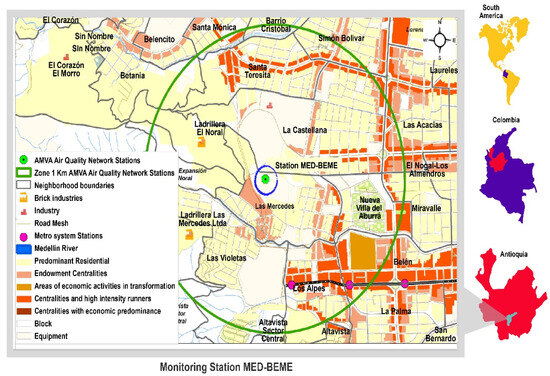
Figure 1.
Geographical location of the MED-BEME station.
Specifically, the monitoring station is located in Belén las Mercedes in Medellín, a residential area with high population density (divided into 21 neighborhoods with a total area of 8.8 km2) and catalogued within the Aburrá Valley Air Quality Network as an urban background zone with low incidence of vehicular sources. Therefore, its level of average contamination is not directly influenced by local sources but by the contribution of emissions influenced by wind transport from the dominant northeastern direction. Thus, the sampling point was selected considering the characteristics of residential areas, with proximity to the heart of the city, large road and public mobility developments, and public and private facilities that impact the entire city.
The land in this region is characterized by gentle to moderate slopes throughout most of its territory, with no direct industrial influence, except for a brick kiln located 620 m away. It experiences medium to light vehicular traffic and less heavy traffic and has dominant secondary and main roads approximately 400 m away in a straight line. The measuring equipment was located within an area of influence of 883.12 hectares, equivalent to 9% of the total urban area and 2.7% of the Medellín city area.
2.2. PM2.5 Analysis
PM2.5 measurements were carried out using EPA CFR 40 Appendix L to Part 50—Reference Method for the Determination of Fine Particulate Matter as PM2.5 in the Atmosphere, according to the air quality monitoring protocol [40]. Samples were collected from 1 December 2018, to 23 November 2020, for a period of 24 ± 1 h and a frequency of three days per week on alternating days, including Saturday and Sunday (Monday, Wednesday, Friday, Sunday, Tuesday, Thursday, Saturday), as these were the days with the greatest variation in city dynamics. A total of 244 validated PM2.5 samples were collected using a low volume meter Tisch Environmental-Wilbur (Manufacturer Tisch Environmental, reference Wilbur. 145 South Miami Avenue | Cleves, OH 45002, United States) with a continuous flow rate of 16.67 L min−1, 47 mm Teflon filters, an automatic control system, and continuous flow regulation according to filter saturation and changes in environmental conditions.
2.3. Data Collection and Systematization Periods
The periods of the COVID-19 pandemic were defined as the main criterion, given the measures that led to the suspension of most activities in the region. Specific analyses were conducted for the period before the pandemic (21 February to 19 March) and during both the strict lockdown (SL) from 20 March to 26 April and the relaxed lockdown (RL) from 27 April to 30 June of the same year, to assess the impact of the restrictive measures on air quality. SL was characterized by an almost total restriction of vehicular traffic and industrial activity, while RL was defined by specific measures affecting the expected behavior of sources, resulting in a significant decrease in mobile and stationary sources (Table 1). It is noteworthy that the typical air quality episodes that occur in the region (AS), which also occurred during the pandemic due to the low dispersion of pollutants, are included (Table 1). These episodes will be part of the assessment of the impact using the artificial intelligence tool, according to the judgment of air quality experts.

Table 1.
Identification and description of each data collection period.
The data were collected from a single representative air quality monitoring station located in a residential area of the Aburrá Valley. In accordance with the objective of evaluating the AI tool, only this control sample was considered to assess the variability and implications of the restrictive measures. The dataset is available at https://drive.google.com/drive/u/3/folders/17nTWJjlKYMaks1b67FWJXKq4kPE4H535 (accessed on 18 January 2025).
2.4. Multivariate Analysis Tool
Classifiers for multivariate analysis can be obtained by several techniques, including artificial intelligence (AI) [21,34,41]. These techniques allow for the identification of classes that, after being approved by experts, represent the functional states of the process or system under study. In addition to the important task of making decisions, knowledge of the functional states allows for a detailed understanding of the relationships between the classes and the descriptors (variables) on the basis of which they are formed [42].
Figure 2 presents a typical framework for data-driven process supervision and diagnosis using classifiers. This data monitoring scheme is shown for the offline training stage, while the process information obtained by physical measurements is stored in a historical file (historical data). In the learning stage, the historical process data are used to train a classifier, which assigns a class to each signal sample or set of descriptors. The historical dataset for this study contains information on five descriptors (PM2.5, management of air quality episodes, PANDEMIC, strict lockdown, and relaxed lockdown) and includes 244 samples. In the learning stage, the historical data of the process are used to train a classifier, which assigns a class to each signal sample or set of descriptors. These classes, after being analyzed by the process expert, are associated with functional states, and it is necessary to determine the actions that are required and should be suggested to the process operator. Monitoring and supervision of each new sample processed by the classifier are carried out online. According to the classification, the corresponding functional state is identified; next, this state and the required actions are presented to the operator. The overall aim is to identify the state of the process at each instant, providing the operator with an analytical element for decision-making.
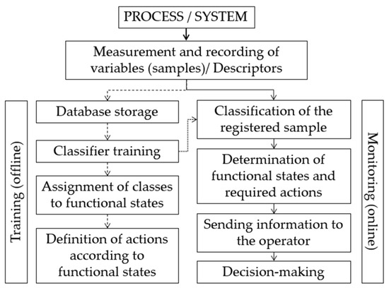
Figure 2.
Data monitoring flow chart used in this study (The dashed arrow indicates the sequence of the offline training, while the solid line represents the sequence of the online monitoring operation).
For this research development, the training stage is carried out using a supervised learning scheme, since the classes or functional states are known. The classifier training will allow us to determine how the different descriptors are associated with the pre-existing states and propose a way to visualize the information related to air quality data (PM2.5) based on the correspondence of classes for each temporal record.
One method used in monitoring and supervision, based on classifiers, is fuzzy clustering. Unlike hard clustering, this technique not only identifies the class or functional state to which the sample belongs but also assesses the degree of membership of a sample in each class or state. These degrees of membership enable the analysis and validation of the classifications [42,43]. Among the classification methods used in monitoring and supervision is the K-means. This is one of the simplest and most popular unsupervised machine learning algorithms, requiring the initial centroids as parameters and the number of class (K) for training [44]. An optimization criterion allows clustering data according to their similarity; in this case, the distance measures the separation of a data point from the center of a class.
Fuzzy C-Means (FCM) is another commonly used method, which is based on the minimization of the Euclidean distance dij (dij =|xi − ci|) between the data of a sample (register), xi, and the centers of classes cj. The value uij in the range [0, 1] represents the degree of membership assigned for each sample, xi, with respect to each class or Cluster j. The minimization function J is defined in terms of the degree of membership matrix U[uij] and the centers cj Equation (1). The class clustering for this method is shaped like hyperspheres [45,46].
Furthermore, the GK-means method, derived from FCM, uses the Mahalanobis dij (dij = (xi − cj)V−1(xi − ci)) distance measurement, where V−1 is the inverse of the covariance matrix and allows making the clustering of classes in the shape of hyperellipsoids [47]. Lastly, the LAMDA method, from its English name “Learning Algorithm Multivariable and Data Analysis” [48], allows working with class updating. Unlike the previous methods, it can process both quantitative and qualitative data and estimate the degree of adaptation of each data point to the classes. Adaptation is established in the possibilistic sense. The Marginal Adequacy Degree (MAD) of each descriptor xj to each class is analyzed by LAMDA. From an interpolation of T-Norm and S-Norm, the global adequacy degree (GAD) of each data point x (set of descriptors or variables in a sampling time) is obtained for each class. For class adequacy, the Non-Informative Class (NIC) is used as the minimum threshold to determine whether an element belongs to a class.
When the descriptor is numerical, the MAD is calculated by selecting one of the different functions, including the fuzzy extension of the binomial function Equation (2) and the Gaussian function Equation (3), which are commonly used.
where xg is the normalized variable, and ρjg corresponds to the mean value for the variable xg in the class j.
where σ is the standard deviation, and m is the mean, and (xg − mjg) the parameter measures the proximity to the prototype. When the descriptor is qualitative, the observed frequency of its attribute modality is used to assess the MAD.
The aggregate function is a linear interpolation between t-norm (γ) and t-conorm (β) as shown in Equation (4), where the parameter α, 0 ≤ α ≤ 1, is called exigency.
where is the vector of normalized registers with n descriptors, and C corresponds to the class (C = [1, 2, …, #classes]).
The most common fuzzy logic operators are {γ(a,b) = a*b; β(a,b) = a + b − a*b} and {γ(a,b) = min(a,b); β(a,b) = max(a,b)}, where a and b are fuzzy values. Each data point x’ is assigned the class C according to the maximum value of GAD.
Isaza et al. [49] conducted a comparative analysis of various representative classification techniques. These included fuzzy clustering methods such as GK-means and LAMDA, radial basis functions for artificial neural networks (ANNs), Fisher linear discriminant, and the k-nearest neighbor method, which represent statistical approaches. In addition, CART decision trees were considered by Breiman et al. [50]. Table 2 summarizes the key characteristics of these classification methods and the parameters defined by the user.
Table 2.
Classification methods: main characteristics, adapted from [49].
For the comparative analysis, four well-known benchmark datasets from the UCI Repository were used: Iris, Australian Credit, Heart Disease, and Wastewater Treatment Plant [51]. The selection of these datasets allowed for a comprehensive evaluation of the LAMDA method across diverse data characteristics. The training datasets selected exhibit high variability in several aspects: dataset size (ranging from 150 to 1000 records), number of classes (from 2 to 13), number of descriptors (from 4 to 38), and the presence of symbolic descriptors. This variability allows for a comprehensive evaluation of the generalization capability of the LAMDA model, which is a significant advantage, as strong generalization performance is crucial for real-world applications beyond the training dataset.
In general, when appropriate parameters were selected, the methods demonstrated acceptable performance in both training and testing phases. However, for the Australian Credit and Wastewater Treatment Plant datasets, achieving a classifier with satisfactory performance was not possible using RBF and GK-means, respectively. In contrast, LAMDA consistently exhibited strong generalization capability, as its test performance closely matched its training performance.
LAMDA offers several advantages, including ease of result interpretation and a fast training algorithm that does not rely on error minimization, yielding results in the first iteration. Additionally, it enables unsupervised classification without requiring a predefined number of classes and can handle mixed data types (qualitative and quantitative). This method not only facilitates knowledge extraction from the training dataset but also allows for the addition of new classes without requiring a new learning phase—an advantage not found in other methods.
LAMDA is frequently compared to GK-means, as both are considered unsupervised learning algorithms. However, GK-means requires a predefined number of classes and is highly sensitive to parameter selection. Moreover, since GK-means is an optimization-based method, its results are significantly influenced by the random initialization of class centers, leading to variability in classification outcomes.
The LAMDA methodology, implemented in the SALSA software [52,53], allows passive recognition, self-learning (which does not require knowing the number of groups in advance), and supervised learning. This technique processes quantitative, qualitative, and interval data, and it is not an iterative algorithm. The recognition classification mode allows the inclusion of a class for each record to be considered when running the algorithm; the learning process ensures that the obtained distribution matches the predefined classification to the extent allowed by the variation of the algorithm parameters [54].
Once the clusters have been defined by fuzzy partitioning, where each group corresponds to a class, it is possible to create transition matrices. These matrices are defined as an array Tj,k, where elements are estimated based on the occurrence of transitions (classes registered in consecutive registers) in the database. The following three (3) transition matrices can be considered:
- A raw transition matrix RT = [RTj k], where RTj k is the number of transitions observed of class j and class k Equation (5). The diagonal terms RTj j indicate the number of records in class j, i.e., the number of instants or recording times the system was in this class.
- Departure graph matrix DT = [DTj, k] Equation (6)
- Arrival graph matrix AT = [ATj, k] Equation (7)
The diagonal terms of the matrices DT and AT are, respectively, the number of outputs from and inputs to a class. From these matrices, it is possible to obtain the graph or automaton where the states correspond to the classes, making it possible to present the information on the dynamics of the system in a visual, simple, and easily understandable way [24,55].
In Figure 2, after “Measurement and Recording of Variables (samples) or Descriptors”, normalization is required to ensure equal importance for each descriptor in the classification. Equation (8) corresponds to the normalization of each descriptor (v), where v_minimum and v_maximum represent the minimum and maximum values of the corresponding descriptor. By applying Equation (8) to each descriptor, all sample values will be scaled within the range [0, 1], including the boundary values 0 and 1.
2.5. Information for Classifier Training
Figure 3 shows the five (5) descriptors used with their respective temporal registers for classifier definition and data analysis. From the temporal register of the data, it can be observed that in the case of the AS descriptor (Figure 3b), four periods were recorded with value 1 due to its occurrence. For the PANDEMIC descriptor (Figure 3c), the event wasstarted from the concentration record of sample 159, with an occurrence value of 1. For the SL descriptor (Figure 3d), the event was recorded a single time and included the smallest number of samples (12 of 244), with an occurrence value of 1. Finally, for the RL descriptor (Figure 3e), the event started from the recording of data number 171, with an occurrence value of 1.
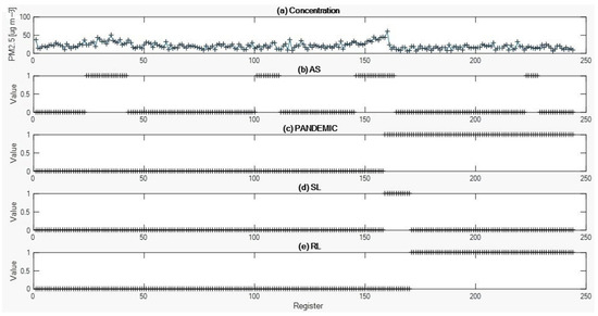
Figure 3.
Descriptors and temporal records used for classifier definition and data analysis. (a) PM2.5 Concentration record vs. Registers, (b) AS vs. Registers, (c) PANDEMIC vs. Registers, (d) SL vs. Registers, and (e) RL vs. Registers (The ‘+’ symbol indicates, for each subfigure, the variable’s value at each temporal record).
Furthermore, in Table 3, the five descriptors and their contexts, i.e., maximum and minimum corresponding values, are presented, which are used for normalization according to Equation (8). The five variables were normalized and then processed in the LAMDA algorithm.
Table 3.
Maximum and minimum values of context defined for each descriptor.
Four classes were defined within which each of the 244 environmental PM2.5 samples was associated according to the cut-off points (concentration) of the AQI established in the environmental regulations [34]. Table 4 shows these classes with their respective ranges and categories of air quality and their effect on health.
Table 4.
Air quality classes, concentration ranges, and categories according to AQI.
The well-known and straightforward methodology for evaluating air quality indicators, such as the air quality index (AQI), is based on existing regulations. However, decision-makers and other non-expert professionals in this field must always keep in mind the standard limits that define the various categories as a criterion for analysis.
As an alternative, using and analyzing classifiers equivalent to the AQI allows for an additional assessment of air quality issues. This method evaluates the frequency of events in each class or category and the transitions between them, especially in relation to how one class increases or decreases compared to another. This makes it possible to estimate the changing exposure time (in days) to specific health risks, which is crucial for health impact studies.
3. Results
Four classes were defined, associating each of the 244 environmental PM2.5 samples according to the cut-off points (concentration) of the AQI established in the environmental regulation [34]. Table 3 indicates these classes with their respective ranges and categories of air quality and their impact on health.
The training was carried out in “recognition” mode, with the classes defined for each record of the historical data of environmental PM2.5 as the basis. This approach analyzed the incidence of the different variables according to compliance with the pre-established classification. Figure 4 presents the results of the recognized classification, where the horizontal axis contains the registration numbers corresponding to calendar dates, and on the vertical axis, the four classes were located according to Table 3.
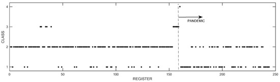
Figure 4.
Results of the recognized classification with temporal data and class distribution (Each black dot represents the assigned class label at a given sampling time, and, the arrow labeled ‘Pandemic’ marks the point at which it started and signifies its continuation in the following records).
By applying the LAMDA algorithm with the required parameter adjustment in recognition mode, it was identified that 85.25% of the records were well-recognized, with each record corresponding to the quintuple of the descriptors (Concentration, AS, PANDEMIC, SL, and RL). This result was achieved using a “fuzzy” extension of the Gaussian function, a MinMax Fuzzy Logic operator, and an exigency value of α = 1. In other words, 208 records out of the total (85.25%) are well classified. The records recognized unsuccessfully were 3, 34, 46, 49, 63, 76, 91, 100, 103, 110, 111, 132, 156, 161, 163, 167, 168, 176, 177, 181, 183, 185, 186, 197, 198, 199, 200, 202, 210, 211, 212, 218, 229, 231, 234, and 241. Subsequently, a detailed analysis of these records was carried out using the fuzzy membership degrees provided by the classifier.
Considering that the highest membership degree per record defines the classification, it was evident that in all these cases, the membership degrees immediately below the corresponding maximum matched the class that should have been recognized. This discrepancy occurs because the PM2.5 value of the monitoring site does not coincide with the average value of the values registered at different sites, which were taken into account for decision-making. Therefore, the AQI category classification of the points close to change in the different records analyzed can be affected. It was validated that for all these cases, the PM2.5 concentration values were close to the limits of the different categories established by the AQI. This indicates that a good classifier was obtained for the PM2.5 database used, distributed in the AS and AI periods, for the PANDEMIC, SL, and RL conditions. From these results, it was possible to analyze the way in which the descriptors affect the classification.
As shown in Table 5, the PM2.5 concentrations fall into the good category (C1, 71 samples), with an average of 11 μg m−3. The AS periods are present in the C1 class, with an average of 0.09, as well as for the PANDEMIC descriptor at 0.59, SL at 0.14, and RL at 0.45.
Table 5.
General class profile information (mean and standard deviation).
Excluding the Concentration descriptor, the mean values less than 1 indicate that the concentration level according to the class occurred in different environmental conditions or associated with the pandemic (Table 1). The mean and standard deviation values determine each of the fuzzy functions that make up the classifier.
The normalized values of the class mean are shown in Figure 5. In the case of the PM2.5 Concentration descriptor, the actual meaning in each class is also included. This demonstrates how these values, as estimated by the classifier, were consistent with the ranges and ascending behavior established for each category by the AQI.
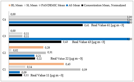
Figure 5.
Normalized class profile based on descriptor values.
The preventive measures taken by the environmental authority are demonstrated by observing AS records in category C1 (mean AS 0.09), which, according to the concentration range, would not typically imply its declaration. The increase in the number of days during which it was mandatory to take additional prevention and control measures—C2 to C4—can be explained by the meteorological characteristics of the region [34].
The impact of the mandatory restrictions during the pandemic was shown by the greater number of days in the C1 good category (mean P 0.59). The effects of the pandemic contributed to improving air quality, as indicated by the ongoing behavior from C1 to C3 (C1 0.59; C2 0.31; and C3 0.11). The behavior of SL should be decreasing by categories, similar to RL, from C1 to C4; however, the presence of regional emissions associated with fires altered this dynamic. The highest concentration value produced by biomass burning appeared in the profile of the harmful to health category—Class C4—which matched the AS, PANDEMIC, and SL periods. Additionally, the classifier results appear evident when comparing the classes and their relationship with each descriptor, showing clearly distinct and well-defined fuzzy partition [55].
4. Discussion
To represent the dynamics of air quality changes during the study period, the Crude Transition Matrix was used according to Equation (5). The results obtained with the classifier are shown in Table 6. As can be seen, during the time between December 2018 and November 2020, there were 71 days with Class 1 (C1) good air quality, later changing to the C2 acceptable category for 36 days (transitions from C1 to C2). There were no changes from Class C1 to the harmful Classes C3 or C4. Analyzing the inline values of the main diagonal, it is observed that the largest number of records (161) were in Class C2 (acceptable). There were eleven records in the harmful to the health of sensitive groups category (C3) and only one record in the harmful to health category (C4).
Table 6.
Matrix of state or category transitions associated with the air quality indexes.
Using the matrix yielded a graph or automaton representation (Figure 6), allowing us to visualize the dynamics of air quality in a simple and easily understandable way during the study. This provides the following findings:
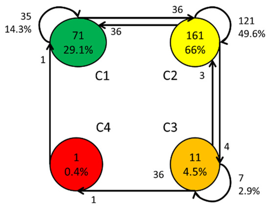
Figure 6.
Class transition and permanence percentages in relation to air quality (the colors indicate air quality according to Table 4, and the arrows represent the direction and trend observed based on the available historical records).
- The good (29.1%) and acceptable (66%) categories remained at 95.1% of the days, which was an important assessment for the community perception of air quality.
- During the majority of records (66%), Class C2 (acceptable category) appeared.
- The harmful to the health of sensitive groups category (C3) included 11 records (4.5%).
- Only one record (0.4%) appeared in the harmful to health category (C4).
Other information displayed in Figure 6 refers to the percentage of class permanence over time and the transition percentage from one class to another. In C1, 29.1% (71 days) were classified as having good air quality with transitions only to C2 (36 records), which returned to C1 in 35 non-consecutive days (14.3%). The largest number of records (161) was assessed as the acceptable category (C2). The air quality improved over 36 days, transitioning to C1; pollution increased to C3 on four days but subsided (C3 to C2) in three days, without reaching the harmful Class C4. Transitions to Class C2 were assessed over 121 days (49.6%). In the C4 harmful to health category, there was only one (1) record registration, and the transition to C1 appeared as a favorable condition.
To analyze the impact of the pandemic, the study period was divided from the date of the COVID-19 declaration emergency (20 March 2020) onward. This same class representation method was applied using the Crude Transition Matrix (Table 7a,b). The graphs or automata corresponding to these matrices are shown in Figure 7. The records of Classes C1 and C2 combined before the pandemic were 93.7% and 97.7% during the pandemic. The improvements in air quality resulting from the restrictions during the health emergency are highlighted, with 57% of the observations corresponding to the good category (C1) during the pandemic vs. 13.9% before the pandemic.
Table 7.
Matrix showing transitions before the pandemic declaration and during the pandemic.
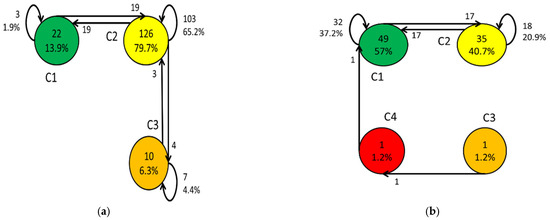
Figure 7.
Class transition and permanence percentages in relation to air quality before (a) and during the pandemic (b); the colors indicate air quality according to Table 4, and the arrows represent the direction and trend observed based on the available historical records.
The results obtained in this research confirm that the isolation measures taken by the Colombian government to control the COVID-19 pandemic positively impacted air quality, decreasing the PM2.5 concentrations in the urban study area due to the overall decrease in air polluting emissions. This study is not the only one to demonstrate air quality improvement in some regions of Colombia during the COVID-19 pandemic; recent research has reported reductions in gases and particulate matter due to decreased vehicle flow and industrial emissions caused by the restrictions on mobility and commercial activities. This result is similar to the findings of many previous studies. For example, Mendez-Espinosa et al. [56] studied variations in air quality in the two most populated cities in Colombia (Bogotá and Medellín) during the quarantine period from 21 February to 30 June 2020. Their analyses showed short-term reductions in the concentration of NO2, PM10, and PM2.5 of 60%, 44%, and 40%, respectively, during mandatory quarantine, and 62%, 58%, and 69% for smart quarantine.
Similarly, Heli A. Arregocés et al. [57] assessed the impact of lockdown measures due to the COVID-19 pandemic on PM2.5 concentrations across five monitoring stations as well as aerosol optical depth values obtained by the Terra/MODIS satellite. Similar to the present study, these researchers observed substantial reductions in weekly PM2.5 concentrations: from 41% to 84% (Bogotá), from 13% to 66% (Funza), from 17% to 57% (Boyacá), from 35% to 86% (Valledupar), and from 31% to 60% (Risaralda). Juan J. Henao et al. [17] studied changes in air pollution levels during the lockdown in Medellín, Colombia, and its metropolitan area for periods with and without enhanced regional fire activity, considering the effects of meteorology using random forest and multiple linear regression methods. Their results showed that the lockdown measures, which reduced mean traffic volume by 70% compared to 2016–2019, resulted in reductions for PM2.5 (50–63%), PM10 (59–64%), NO (75–76%), NO2 (43–47%), and CO (40–47%), while O3 concentration increased by 19–22%.
Although research worldwide shows that the increase in air quality during mandatory confinement measures due to the COVID-19 global health emergency is associated with decreased transport and industrial emissions, it is also important to mention that both in the present study and in others examining the same region, an increase in the levels of particulate matter (PM2.5) was also identified during the pandemic [56,57,58]. This was related to environmental factors, such as forest fires of the geographic territory, confirming that the presence of a variety of complex events can significantly affect the atmosphere composition. Thus, in the present research, only one event was recorded for the harmful Classes C3 and C4 (pandemic). This event was caused by biomass fires in the northern and eastern areas of the country and in the Brazilian Amazon.
The findings of this study highlight the immediate effects of COVID-19 restrictions on PM2.5 levels; however, understanding long-term trends in air quality remains crucial for evaluating persistent changes and policy effectiveness. Future research should focus on monitoring air quality over extended periods, particularly analyzing the transition to C3 and C4 pollution categories and their correlation with meteorological and atmospheric events that influence pollutant dispersion in the Aburrá Valley. A more detailed investigation into these long-term trends, including the chemical composition of PM2.5 and source contributions, is presented in a forthcoming study covering the period from 2019 to 2022.
Similar events were identified on the same date in studies carried out by Mendez-Espinosa et al. [56] and Heli A. Arregocés et al. [57]. For example, Mendez-Espinosa et al. [56] observed that the regional biomass indicator increased PM2.5 concentrations by 20 μg m−3 during mandatory confinement measures. Similarly, the Sahara dust event increased PM10 concentrations to 168 μg m−3 in Bogotá and 104 μg m−3 in Medellín, prompting the government to announce additional morbidity and mortality risk levels for the population. Additionally, Heli A. Arregocés et al. [57,58] showed that during the week of 22 June 2020, the optical depth values of atmospheric aerosols were higher compared to the other weeks of the analysis, which they attributed to the Sahara dust masses that crossed the Atlantic Ocean during that time.
The impact of the restrictions (SL and RL) imposed in response to the COVID-19 health emergency is evident when observing an increase in good air quality records from 13.9% to 57% and a decrease from 79.7% to 40.7% on days with acceptable air quality. Likewise, this acceptable category remained the same for 20.9% during the pandemic, with a transition to the C1 good category for 19.8%. There were no transitions to the Harmful Categories C3 and C4. Regarding the health of sensitive groups C3 category, the reduction in registrations from 6.3% (ten records) to 1.2% (one record) before and during the pandemic, respectively, is notable. The transition from C3 to C4 (harmful to health) happened on 25 March, with evidence of regional aerosol transport events resulting from biomass fires; this phenomenon has also been described in previous research [26,32,56,57,59]. Once these fires were extinguished, a transition to C1 occurred.
From our literature review, we understand that no work has been carried out using this specific tool (multivariate clustering method) to determine air quality in Colombia. Therefore, it is not possible to compare our results with those obtained by other researchers. However, in the field of machine learning, new approaches have been successfully implemented to evaluate air quality. For instance, Alejandro Casallas et al. [4] used a long short-term memory artificial neural network approach to forecast meteorology and PM2.5 local variables in Bogotá, Colombia. The researchers concluded that the predictions related to PM2.5, radiation, temperature, relative humidity, and wind speed show good and excellent performance in a city with complex terrain, according to the evaluation parameters and the benchmarks used to compare the results. Additionally, Londoño Pineda and Cano [6] applied a composite air quality index (CAQIAV) to evaluate air quality in the Aburrá Valley. Using a multi-criteria methodology consisting of a framework for the selection, normalization, weighting, and aggregation of indicators to construct the index, they proposed several guidelines and solutions to configure a comprehensive sustainable development policy in this city. Finally, similar studies have been conducted in other countries to build regression models for predicting the AQI or determining the current state of pollution in the atmosphere [9,16].
Although it was expected that PM2.5 concentrations would decrease due to the COVID-19 pandemic measures, this article aims to demonstrate not just this effect but also the opportunity to use other indicators beyond the AQI to evaluate the impact of specific events affecting air quality. In this context, the formation of data classes from temporal PM2.5 records, using artificial intelligence tools, provides a straightforward and visual (graphical) representation of both current and dynamic knowledge of air quality in the study region under similar conditions.
The experience of using classifiers for PM2.5 concentrations and other air quality data can also be applied to the continuous programming of alarms. These alarms alert to health-dangerous values related to nearby locations or events, such as biomass burning, Sahara dust transport, and particularly during frequent periods of atmospheric stability in the region (AE).
Parra et al. [60] analyzed the impact of various environmental factors influencing PM2.5 levels, considering meteorological conditions, seasonal variations, and industrial activities in the region.
The long-term implications of these findings highlight the need for future research to monitor air quality over extended periods, focusing on transitions to C3 and C4 categories (harmful to health) and their correlation with atmospheric events affecting the Aburrá Valley.
The use of classifiers for PM2.5 concentrations and other air quality issues can facilitate the continuous programming of alarms during peak pollution events. These alarms are particularly relevant in mountainous climates, where emission variability, combined with seasonal transitions from dry to rainy periods, exacerbates pollution levels. Such warnings can help mitigate health risks associated with biomass burning, Saharan dust transport, and frequent periods of atmospheric stability in the region.
By classifying air quality data based on health impact, this approach provides environmental authorities with valuable insights for managing emissions and evaluating the effectiveness of air quality improvement measures. Systematic monitoring of these classifiers will support decision-making by integrating cross-referenced data from emission inventories, chemical characterization, meteorology, and satellite reports, contributing to a comprehensive framework for environmental data management [61].
Future studies should extend this methodology to all monitoring stations in the region, leveraging advances in the analysis of PM2.5 emission sources, ambient conditions, and vehicular activity. Additionally, incorporating physical and chemical processes governing secondary aerosol formation will enhance the accuracy of predictive models and policy recommendations.
5. Conclusions
The results obtained demonstrate the improvement in air quality resulting from the restrictions during the health emergency, highlighted by 57% of observations corresponding to the good category (C1) during the pandemic, compared to 13.9% before the pandemic. In contrast to other AQI methods, the multivariate clustering methodology allows us to evaluate that the acceptable category remained the same at 20.9% during the pandemic, with a transition to the C1 good category at 19.8%, and there were no transitions to the Harmful Categories C3 and C4. The reduction in the Health of Sensitive Groups C3 is notable, with registrations decreasing from 6.3% (ten records) to 1.2% (one record) before and during the pandemic, respectively.
The LAMDA methodology implemented in recognition mode enabled the development of a classifier according to the AQI classes for the records stored between 2018 and 2021. These variables or descriptors included PM2.5 concentration levels, the presence or absence of the COVID-19 pandemic, declared periods of environmental management, and periods with mandatory and flexible preventive quarantine measures. It is proposed to use the trained classifier, or retrain it with an expanded database, to fulfill its role in the ongoing monitoring (new records of variables or descriptors) of air quality in the study area and to evaluate its potential for use in a predictive scheme.
Unlike traditional methods used in air quality analysis, this technique allows for the determination of the frequency of events in each class or category and the transitions between them. Therefore, with sufficient training data and historical air quality records provided by the classifier, it is possible to forecast the risk of reaching the AQI category harmful to the health of sensitive groups (C3) in a relatively short period of time. This technique serves as a management tool for implementing immediate measures to reduce pollutant emissions, such as the implementation of environmental restriction measures known as “pico y placa ambiental”, creating a rapid, accurate, and applicable tool for managing air pollution events.
A supervision system based on a classifier trained with LAMDA would allow the identification of the corresponding current class according to the input records. Moreover, this classifier could be used in a class prediction approach similar to the one proposed in a study [62]. In that methodology, the fuzzy membership degrees obtained through LAMDA are essential. However, even without a prediction framework, the membership degrees—where the highest value determines the current class—offer a trend analysis tool for decision-making. Given that records are generated every two days, there would be sufficient time to analyze class trends and behaviors, incorporating exogenous information that may be relevant.
6. Future Research and Challenges
The use of classifiers for PM2.5 concentrations and other air quality issues facilitates the continuous programming of alarms during peak pollution events. These alarms are particularly relevant in mountainous climates, where emission variability, seasonal transitions, and atmospheric stability exacerbate pollution levels. Such warnings help mitigate health risks associated with biomass burning, Saharan dust transport, and other episodic pollution sources.
By classifying air quality data based on health impact, this approach provides environmental authorities with valuable insights for managing emissions and evaluating air quality improvement measures. Systematic monitoring of classifiers supports decision-making by integrating cross-referenced data from emission inventories, chemical characterization, meteorology, and satellite observations, contributing to a comprehensive framework for environmental data management.
Future research should extend this methodology to all monitoring stations in the region, enabling a broader assessment of spatial and temporal air quality trends. Advances in the analysis of PM2.5 emission sources, atmospheric conditions, and vehicular activity will enhance predictive capabilities, allowing policymakers to anticipate pollution episodes and optimize control measures. Additionally, incorporating physical and chemical processes governing secondary aerosol formation will refine predictive models and strengthen regulatory frameworks.
The application of artificial intelligence tools in air quality analysis offers a novel framework for evaluating pollution levels based on health impact. By utilizing data classifiers, authorities can systematically track air quality index (AQI) variations as an indicator of the effectiveness of management strategies. This methodological approach enables the integration of diverse datasets, facilitating a deeper understanding of air pollution dynamics. A conceptual architectural solution for data integration, as proposed by Vergara-Correa et al. [61], could enhance the development of robust air quality management indicators, improving real-time evaluation of interventions.
In the context of future pandemics or other large-scale disruptions, this approach could provide rapid insights into the effects of emergency measures, supporting adaptive responses to mitigate air pollution and protect public health. AI-driven analysis presents a valuable ospportunity to strengthen evidence-based environmental governance, ensuring that air quality policies remain responsive to both routine conditions and crisis scenarios.
Author Contributions
Conceptualization: M.G.M., H.O.S.-M., A.N.A.A., W.A.G.A. and R.D.V.-S.; methodology: M.G.M., H.O.S.-M. and A.N.A.A.; validation: H.O.S.-M.; formal analysis: M.G.M. and H.O.S.-M.; investigation: M.G.M.; resources: M.G.M., H.O.S.-M. and A.N.A.A.; data curation: writing—preparation of the original draft: M.G.M., H.O.S.-M. and A.N.A.A.; writing—review and editing: M.G.M., H.O.S.-M. and A.N.A.A.; visualization, supervision: M.G.M.; project administration: M.G.M.; acquisition of financing: M.G.M. All authors have read and agreed to the published version of the manuscript.
Funding
The authors are grateful to the Colombian Ministry of Science, Technology, and Innovation (grant no. 2020000100410) for funding the PM2:5 chemical composition sampling campaign; United Nations International Atomic Energy Agency (IAEA), the Metropolitan Area in the Aburrá Valley (AMVA), Ecopetrol and Politécnico Colombiano Jaime Isaza Cadavid for financing the ARCAL RLA 7023.
Informed Consent Statement
Not applicable.
Data Availability Statement
The available data of this study can be downloaded at: https://drive.google.com/drive/u/3/folders/17nTWJjlKYMaks1b67FWJXKq4kPE4H535 (accessed on 21 January 2025).
Acknowledgments
The authors would like to thank the acknowledge for funding the PM2:5 chemical composition sampling campaign to the Colombian Ministry of Science, Technology, and Innovation (grant no. 2020000100410) for funding the PM2:5 chemical composition sampling campaign; United Nations International Atomic Energy Agency (IAEA), the Metropolitan Area in the Aburrá Valley (AMVA), and Ecopetrol and Politécnico Colombiano Jaime Isaza Cadavid for financing the ARCAL RLA 7023 Project for the Latin American atmospheric basin ranging from Argentina to Mexico. The project “Evaluación de componentes de aerosoles en áreas urbanas, para mejorar la gestión de la contaminación del aire y de cambio climático,” is currently developing a pilot in the Aburrá Valley in Colombia. This initiative recognizes the importance of decision-making capabilities based on technical and scientific understanding of atmospheric aerosols and their emission sources.
Conflicts of Interest
The authors declare that they have no known competing financial interests or personal relationships that could have appeared to influence the work reported in this paper.
References
- Kumari, S.; Jain, M.K. A Critical Review on Air Quality Index. Environ. Pollut. 2018, 87–102. [Google Scholar] [CrossRef]
- Janarthanan, R.; Partheeban, P.; Somasundaram, K.; Navin Elamparithi, P. A Deep Learning Approach for Prediction of Air Quality Index in a Metropolitan City. Sustain. Cities Soc. 2021, 67, 102720. [Google Scholar] [CrossRef]
- Gope, S.; Dawn, S.; Das, S.S. Effect of COVID-19 Pandemic on Air Quality: A Study Based on Air Quality Index. Environ. Sci. Pollut. Res. 2021, 28, 35564–35583. [Google Scholar] [CrossRef] [PubMed]
- Casallas, A.; Ferro, C.; Celis, N.; Guevara-Luna, M.A.; Mogollón-Sotelo, C.; Guevara-Luna, F.A.; Merchán, M. Long Short-Term Memory Artificial Neural Network Approach to Forecast Meteorology and PM2.5 Local Variables in Bogotá, Colombia. Model. Earth Syst. Environ. 2022, 8, 2951–2964. [Google Scholar] [CrossRef]
- Zeng, J.; Wang, C. Temporal Characteristics and Spatial Heterogeneity of Air Quality Changes Due to the COVID-19 Lockdown in China. Resour. Conserv. Recycl. 2022, 181, 106223. [Google Scholar] [CrossRef]
- Londoño Pineda, A.A.; Cano, J.A. Assessment of Air Quality in the Aburrá Valley (Colombia) Using Composite Indices: Towards Comprehensive Sustainable Development Planning. Urban Clim. 2021, 39, 100942. [Google Scholar] [CrossRef]
- Sahraei, M.A.; Kuşkapan, E.; Çodur, M.Y. Public Transit Usage and Air Quality Index during the COVID-19 Lockdown. J. Environ. Manag. 2021, 286, 112166. [Google Scholar] [CrossRef]
- Xu, K.; Cui, K.; Young, L.H.; Wang, Y.F.; Hsieh, Y.K.; Wan, S.; Zhang, J. Air Quality Index, Indicatory Air Pollutants and Impact of COVID-19 Event on the Air Quality near Central China. Aerosol Air Qual. Res. 2020, 20, 1204–1221. [Google Scholar] [CrossRef]
- Liu, H.; Li, Q.; Yu, D.; Gu, Y. Air Quality Index and Air Pollutant Concentration Prediction Based on Machine Learning Algorithms. Appl. Sci. 2019, 9, 4069. [Google Scholar] [CrossRef]
- Perlmutt, L.D.; Cromar, K.R. Comparing Associations of Respiratory Risk for the EPA Air Quality Index and Health-Based Air Quality Indices. Atmos. Environ. 2019, 202, 1–7. [Google Scholar] [CrossRef]
- Borbet, T.C.; Gladson, L.A.; Cromar, K.R. Assessing Air Quality Index Awareness and Use in Mexico City. BMC Public Health 2018, 18, 538. [Google Scholar] [CrossRef] [PubMed]
- Monforte, P.; Ragusa, M.A. Evaluation of the Air Pollution in a Mediterranean Region by the Air Quality Index. Environ. Monit. Assess. 2018, 190, 625. [Google Scholar] [CrossRef] [PubMed]
- Zhu, S.; Lian, X.; Liu, H.; Hu, J.; Wang, Y.; Che, J. Daily Air Quality Index Forecasting with Hybrid Models: A Case in China. Environ. Pollut. 2017, 231, 1232–1244. [Google Scholar] [CrossRef] [PubMed]
- Benchrif, A.; Wheida, A.; Tahri, M.; Shubbar, R.M.; Biswas, B. Air Quality during Three COVID-19 Lockdown Phases: AQI, PM2.5 and NO2 Assessment in Cities with More than 1 Million Inhabitants. Sustain. Cities Soc. 2021, 74, 103170. [Google Scholar] [CrossRef]
- Rodríguez-Urrego, D.; Rodríguez-Urrego, L. Air Quality during the COVID-19: PM2.5 Analysis in the 50 Most Polluted Capital Cities in the World. Environ. Pollut. 2020, 266, 115042. [Google Scholar] [CrossRef]
- Lin, Y.C.; Lee, S.J.; Ouyang, C.; Sen; Wu, C.H. Air Quality Prediction by Neuro-Fuzzy Modeling Approach. Appl. Soft Comput. J. 2020, 86, 105898. [Google Scholar] [CrossRef]
- Henao, J.J.; Rendón, A.M.; Hernández, K.S.; Giraldo-Ramirez, P.A.; Robledo, V.; Posada-Marín, J.A.; Bernal, N.; Salazar, J.F.; Mejía, J.F. Differential Effects of the COVID-19 Lockdown and Regional Fire on the Air Quality of Medellín, Colombia. Atmosphere. 2021, 12, 1137. [Google Scholar] [CrossRef]
- Jin, Z.; Velásquez Angel, M.A.; Mura, I.; Franco, J.F. Enriched spatial analysis of air pollution: Application to the city of Bogotá, Colombia. Front. Environ. Sci. 2022, 10, 966560. [Google Scholar] [CrossRef]
- Luna, G.; Alejandro, F.; Luna, G.; Andrés, M.; Roa, R.; Yezid, N. Spatial-Temporal Assessment and Mapping of the Air Quality and Noise Pollution in a Sub-Area Local Environment inside the Center of a Latin American Megacity: Universidad Nacional de Colombia—Bogotá Campus. Asian J. Atmos. Environ. 2018, 12, 232–243. [Google Scholar] [CrossRef]
- Carriazo, F.; Gomez-Mahecha, J.A. The Demand for Air Quality: Evidence from the Housing Market in Bogotá, Colombia. Environ. Dev. Econ. 2018, 23, 121–138. [Google Scholar] [CrossRef]
- Jaiawei, H.; Micheline, K.; Jian, P. The Morgan Kaufmann Series in Data Management Systems; Morgan Kaufmann: Burlington, MA, USA, 2012; ISBN 9780769550138. [Google Scholar]
- Gore, R.W.; Deshpande, D.S. Voting Method for AQI Prediction and Monitoring Air Pollution using Real-Time Data. In Proceedings of the 2020 International Conference on Smart Innovations in Design, Environment, Management, Planning and Computing (ICSIDEMPC), Aurangabad, India, 30–31 October 2020; pp. 196–199. [Google Scholar] [CrossRef]
- Liu, D.; Veeramachaneni, K.; Geiger, A.; Li, V.O.K.; Qu, H. AQEyes: Visual Analytics for Anomaly Detection and Examination of Air Quality Data. arXiv 2021, arXiv:2103.12910. [Google Scholar]
- Zhang, H.; Ren, K.; Lin, Y.; Qu, D.; Li, Z. AirInsight: Visual Exploration and Interpretation of Latent Patterns and Anomalies in Air Quality Data. Sustainability 2019, 11, 2944. [Google Scholar] [CrossRef]
- Dutta, J.; Gazi, F.; Roy, S.; Chowdhury, C. AirSense: Opportunistic Crowd-Sensing Based Air Quality Monitoring System for Smart City. In Proceedings of the IEEE Sensors, Orlando, FL, USA, 30 October 2016–3 November 2016; pp. 1–3. [Google Scholar] [CrossRef]
- Konduri, P.S.; Kumar, B.R.; Narla, M. Machine Learning Techniques Used for Analysis of Air Quality. Int. J. Comput. Sci. Technol. 2019, 10, 27–31. [Google Scholar]
- Kuo, Y.-H.; Fujiwara, T.; Chou, C.C.-K.; Chen, C.-H.; Ma, K.-L. A Machine-learning-Aided Visual Analysis Workflow for Investigating Air Pollution Data. In Proceedings of the 2022 IEEE 15th Pacific Visualization Symposium (PacificVis), Tsukuba, Japan, 11–14 April 2022; pp. 91–100. [Google Scholar] [CrossRef]
- Deshpande, A. Fuzzy Logic in Air Pollution: Revisited. Nepal J. Environ. Sci. 2014, 2, 1–5. [Google Scholar] [CrossRef]
- Lee, C.; Lee, Z.; Huang, J.; Ye, F.; Ning, Z. Applied Sciences Urban Air Quality Analysis and Forecast Based on Intelligent Algorithm with Parameter Optimization and Decision Rules. Appl. Sci. 2019, 9, 5445. [Google Scholar] [CrossRef]
- Network, C.N.; Images, S. Estimation of Ground PM2.5 Concentrations in Pakistan Using Convolutional Neural Network and Multi-Pollutant Satellite Images. Remote Sens. 2022, 14, 1735. [Google Scholar] [CrossRef]
- Yang, R.; Yan, F.; Zhao, N. Urban Air Quality Based on Bayesian Network. In Proceedings of the 2017 IEEE 9th International Conference on Communication Software and Networks (ICCSN). LOCATION OF CONFERENCE, Guangzhou, China, 6–8 May 2017; pp. 1003–1006. [Google Scholar]
- Rahman, M.M.; Paul, K.C.; Hossain, M.A.; Ali, G.G.M.N.; Rahman, M.S.; Thill, J.C. Machine Learning on the COVID-19 Pandemic, Human Mobility and Air Quality: A Review. IEEE Access 2021, 9, 72420–72450. [Google Scholar] [CrossRef]
- Zhang, J.; Lim, Y.H.; Andersen, Z.J.; Napolitano, G.; Taghavi Shahri, S.M.; So, R.; Plucker, M.; Danesh-Yazdi, M.; Cole-Hunter, T.; Therming Jørgensen, J.; et al. Stringency of COVID-19 Containment Response Policies and Air Quality Changes: A Global Analysis across 1851 Cities. Environ. Sci. Technol. 2022, 56, 12086–12096. [Google Scholar] [CrossRef]
- Ministerio de Ambiente y Desarrollo-Sostenible Resolución 2254 de 2017—Niveles Calidad Del Aire. 2017; pp. 1–11. Available online: https://www.minambiente.gov.co/wp-content/uploads/2021/10/Resolucion-2254-de-2017.pdf (accessed on 2 January 2025).
- De Gennaro, G.; Trizio, L.; Di Gilio, A.; Pey, J.; Pérez, N.; Cusack, M.; Alastuey, A.; Querol, X. Neural Network Model for the Prediction of PM10 Daily Concentrations in Two Sites in the Western Mediterranean. Sci. Total Environ. 2013, 463–464, 875–883. [Google Scholar] [CrossRef]
- Sarkhosh, M.; Najafpoor, A.A.; Alidadi, H.; Shamsara, J.; Amiri, H.; Andrea, T.; Kariminejad, F. Indoor Air Quality Associations with Sick Building Syndrome: An Application of Decision Tree Technology. Build. Environ. 2021, 188, 107446. [Google Scholar] [CrossRef]
- Liu, W.; Guo, G.; Chen, F.; Chen, Y. Meteorological Pattern Analysis Assisted Daily PM2.5 Grades Prediction Using SVM Optimized by PSO Algorithm. Atmos. Pollut. Res. 2019, 10, 1482–1491. [Google Scholar] [CrossRef]
- Keramat-Jahromi, M.; Mohtasebi, S.S.; Mousazadeh, H.; Ghasemi-Varnamkhasti, M.; Rahimi-Movassagh, M. Real-Time Moisture Ratio Study of Drying Date Fruit Chips Based on on-Line Image Attributes Using KNN and Random Forest Regression Methods. Meas. J. Int. Meas. Confed. 2021, 172, 108899. [Google Scholar] [CrossRef]
- Mohammadi, F.; Teiri, H.; Hajizadeh, Y.; Abdolahnejad, A.; Ebrahimi, A. Prediction of Atmospheric PM 2.5 Level by Machine Learning Techniques in Isfahan, Iran. Sci. Rep. 2024, 14, 2109. [Google Scholar] [CrossRef]
- US EPA. CFR Appendix J to Part 50-Reference Method for the Determination of Particulate Matter as PM 10 in the Atmosphere, and Appendix L to Part 50-Reference Method for the Determination of Fine Particulate Matter as PM 2.5 in the Atmosphere; Government Printing Office: Washington, DC, USA, 1997.
- Saxena, A.; Prasad, M.; Gupta, A.; Bharill, N.; Patel, O.P.; Tiwari, A.; Er, M.J.; Ding, W.; Lin, C.-T. A Review of Clustering Techniques and Developments. Neurocomputing 2017, 267, 664–681. [Google Scholar] [CrossRef]
- Isaza, C.; Diez-Lledo, E.; De Leon, H.H.; Aguilar-Martin, J.; Le Lann, M.V. Decision Method for States Validation in Drinking Water Plant Monitoring. IFAC Proc. 2007, 40, 363–368. [Google Scholar] [CrossRef]
- Aguilar-Martin, J. Inteligencia Artificial Para La Supervisión de Procesos Industrial; Laboratorio de Sistemas Inteligentes de la ULA: Caracas, Venezuela, 2007; ISBN 978-980-11-1030-9. [Google Scholar]
- Marroquín, J.L.; Girosi, F. Some Extensions of the k-Means Algorithm for Image Segmentation and Pattern Classification (AI Memo No. 1390); Massachusetts Institute of Technology, Artificial Intelligence Laboratory: Cambridge, MA, USA, 1993. [Google Scholar]
- Ali, M.A.; Dooley, L.S. Review on Fuzzy Clustering Algorithms Journal of Advanced Computations. Open Res. Online 2008, 2, 169–181. [Google Scholar] [CrossRef]
- Lee, D.-J.; Lee, J.-P.; Ji, P.-S.; Park, J.-W.; Lim, J.-Y. Fault Diagnosis of Power Transformer Using SVM and FCM. In Proceedings of the Conference Record of the 2008 IEEE International Symposium on Electrical Insulation, Vancouver, BC, Canada, 9–12 June 2008; pp. 112–115. [Google Scholar]
- Lv, N.; Yu, X.; Wu, J. A Fault Diagnosis Model through G-K Fuzzy Clustering. In Proceedings of the 2004 IEEE International Conference on Systems, Man and Cybernetics, The Hague, The Netherlands, 10–13 October 2004; Volume 6, pp. 5114–5118. [Google Scholar]
- Aguilar Martín, J.; Lopez, R. The Process of Classification and Learning the Meaning of Linguistic Descriptors of Concepts. Approximate Reasoning in Decision Analysis. North Holl. 1982, 1, 165–175. [Google Scholar]
- Isaza, C.V.; Orantes, A.; Kempowsky-hamon, T.; Lann, M. Le Contribution of Fuzzy Classification for the Diagnosis of Complex Systems. IFAC Proc. Vol. 2009, 42, 1132–1137. [Google Scholar] [CrossRef]
- Breiman, L.; Friedman, J.; Olshen, R.A.; Stone, C.J. Classification and Regression Trees, 1st ed.; Chapman and Hall: London, UK, 1984; ISBN 9781315139470. [Google Scholar]
- Markelle, K.; Rachel, L.; Kolby, N. The UCI Machine Learning Repository. Available online: https://archive.ics.uci.edu (accessed on 2 January 2025).
- Alameda-Pineda, X.; Staiano, J.; Ramanathan, S.; Batrinca, L.M.; Ricci, E.; Lepri, B.; Lanz, O.; Sebe, N. SALSA: A Novel Dataset for Multimodal Group Behavior Analysis. IEEE Trans. Pattern Anal. Mach. Intell. 2016, 38, 1707–1720. [Google Scholar] [CrossRef]
- José, A.; Gómez, R.; Strand, P.; Michael, B.; Strand, P.; Chetumal, I.T. The Machine Learning in the Prediction of Elections. ReCIBE Rev. Electrón. Comput. Inform. Bioméd. Electrón. 2015, 4, 4. [Google Scholar]
- Hedjazi, L.; Kempowsky, T.; Despenes, L.; Le Lann, M.-V.; Elgue, S.; Aguilar-Martin, J. Sensor Placement and Fault Detection Using an Efficient Fuzzy Feature Selection Approach. In Proceedings of the 49th IEEE Conference on Decision and Control (CDC), Atlanta, GA, USA, 15–17 December 2010. [Google Scholar]
- Kempowsky, T.; Subias, A.; Aguilar-Martin, J. Process Situation Assessment: From a Fuzzy Partition to a Finite State Machine. Eng. Appl. Artif. Intell. 2006, 19, 461–477. [Google Scholar] [CrossRef]
- Mendez-Espinosa, J.F.; Rojas, N.Y.; Vargas, J.; Pachón, J.E.; Belalcazar, L.C.; Ramírez, O. Air Quality Variations in Northern South America during the COVID-19 Lockdown. Sci. Total Environ. 2020, 749, 141621. [Google Scholar] [CrossRef] [PubMed]
- Arregocés, H.A.; Rojano, R.; Restrepo, G. Impact of Lockdown on Particulate Matter Concentrations in Colombia during the COVID-19 Pandemic. Sci. Total Environ. 2021, 764, 142874. [Google Scholar] [CrossRef] [PubMed]
- Arregoces Reinoso, H.; Rojano Alvarado, R.; Restrepo, G. Effects of Lockdown Due to the COVID-19 Pandemic on Air Quality at Latin America’s Largest Open-Pit Coal Mine. Aerosol Air Qual. Res. 2021, 21, 1–14. [Google Scholar] [CrossRef]
- Coccia, M. The Effects of Atmospheric Stability with Low Wind Speed and of Air Pollution on the Accelerated Transmission Dynamics of COVID-19. Int. J. Environ. Stud. 2021, 78, 1–27. [Google Scholar] [CrossRef]
- Parra, J.C.; Gómez, M.; Salas, H.D.; Botero, B.A.; Piñeros, J.G.; Tavera, J.; Velásquez, M.P. Linking Meteorological Variables and Particulate Matter PM 2.5 in the Aburrá Valley, Colombia. Sustainability 2024, 16, 10250. [Google Scholar] [CrossRef]
- Vergara-Correa, J.A.; Giraldo Plaza, J.E.; Gómez-Marín, M.; Holguín-Marín, J.P.; Montealegre-Hernández, N.A.; Piñeros-Jiménez, J.G. Uso de Arquitectura Dirigida Por Modelos En El Almacenamiento de Datos de PM 2.5 y Salud Pública. Ing. Compet. 2024, 26, 1–16. [Google Scholar] [CrossRef]
- Sarmiento, H.; Isaza, C.; Kempowsky-Hamon, T. Functional State Estimation Methodology Based on Fuzzy Clustering for Complex Process Monitoring BT—Advances in Artificial Intelligence—IBERAMIA 2012; Pavón, J., Duque-Méndez, N.D., Fuentes-Fernández, R., Eds.; Springer: Berlin/Heidelberg, Germany, 2012; pp. 340–349. [Google Scholar]
Disclaimer/Publisher’s Note: The statements, opinions and data contained in all publications are solely those of the individual author(s) and contributor(s) and not of MDPI and/or the editor(s). MDPI and/or the editor(s) disclaim responsibility for any injury to people or property resulting from any ideas, methods, instructions or products referred to in the content. |
© 2025 by the authors. Licensee MDPI, Basel, Switzerland. This article is an open access article distributed under the terms and conditions of the Creative Commons Attribution (CC BY) license (https://creativecommons.org/licenses/by/4.0/).