Identification and Correction for Sun Glint Contamination in Microwave Radiation Imager-Rainfall Mission Global Ocean Observations Onboard the FY-3G Satellite

Abstract

Microwave radiometers are vital for global ocean observations, yet they are prone to errors from radio frequency interference, sun glint, and other contamination. This paper focuses on the newly launched Chinese FY-3G satellite’s Microwave Radiation Imager-Rainfall Mission (MWRI-RM) instrument, aiming to detect sun glint contamination and set a critical angle for data quality control. The model regression difference method is employed to simulate uncontaminated brightness temperatures at 10.65 GHz. By comparing the observed and simulated values, this study finds that sun glint contamination, which causes a 0–5 K increase in brightness temperature, is strongly related to sun glint angle. Based on the statistical analysis of contaminated pixels from November 2023 to July 2024, it is recommended that a critical angle of 25° be used to flag contaminated areas. The method also identifies persistent television frequency interference along the U.S. coastline at 18.7 GHz, which the radio frequency interference (RFI) Flag in Level 1 data failed to detect. Through the utilization of the model regression difference method, the warm biases in the MWRI-RM observations can be corrected. This research offers a practical way to enhance the accuracy of the MWRI-RM data and can be applied to other microwave radiometry missions.

1. Introduction

Over the past several decades, microwave radiometers aboard polar-orbiting meteorological satellites have witnessed significant advancements due to their distinctive technical benefits. The U.S. Defense Meteorological Satellite Program (DMSP) initially carried a series of Special Sensor Microwave/Imager (SSM/I) instruments in 1997 [1]. Subsequent milestones in satellite-based microwave observation included the implementation of the TRMM Microwave Imager (TMI) aboard the Tropical Rainfall Measuring Mission (TRMM) Satellite, followed by the Advanced Microwave Scanning Radiometer-EOS (AMSR-E) onboard the NASA’s Earth Observation System Aqua satellite, and the WindSat Polarimetric Radiometer (Wind-Sat) onboard the U.S. Department of Defense Coriolis experimental satellite [2,3,4]. Microwave Sounding Units (MSUs) and Advanced Microwave Sounding Units (AMSUs) have primarily served the numerical weather prediction modeling community for over thirty years [5]. In 2014, the Global Precipitation Measurement (GPM) core observatory was launched, which carries the GPM Microwave Imager (GMI) as its primary observational instrument [6]. China’s Fengyun-3 satellite program has achieved progress since the launch of the FY-3A satellite in 2008, with seven satellites (FY-3A through FY-3G) currently operational. Among these, all satellites except the FY-3E satellite are equipped with Microwave Radiation Imagers (MWRIs) that significantly enhance Earth observation capabilities [7]. Beyond its conventional use in meteorological satellites for atmospheric monitoring, microwave radiometry exhibits broad applications in diverse fields: (a) fire detection in moving vehicles, (b) planetary exploration, and (c) terrestrial hydrological monitoring [8,9,10].

Ensuring the precision of space-borne passive microwave measurements constitutes a critical prerequisite prior to their utilization in geophysical parameter retrieval, as uncorrected biases propagate to significant errors in derived products. Localized anomalous increases in brightness temperature have often been documented in Level-1B data profiles from the aforementioned microwave radiometers. The high-value observations in brightness temperature measurements are largely caused by radio frequency interference (RFI) contamination. RFI occurs when passive microwave thermal emissions measured by satellites, which are naturally emitted by the surface and atmosphere, become mixed with signals from active sensors [11]. Since space-based microwave radiometers operate their channels in unprotected spectral ranges, RFI significantly influences the accuracy of measurement. This electromagnetic interference induces systematic overestimation of observed brightness temperatures relative to natural emission levels, introducing substantial errors in retrieved geophysical parameters, including sea surface temperature, sea surface wind, soil moisture, and so on [12,13]. Effective detection and mitigation of RFI represent an essential operational requirement, as residual contamination would critically compromise the scientific validity of current and prospective microwave radiometry missions.

Moreover, the Sun serves as the dominant radiative source across the entire electromagnetic spectrum. Sun glint, which is the solar radiation reflected from the ocean surface, introduces warm biases in brightness temperature measurements [14]. Existing studies have documented such contamination effects on SSMIS and TMI observations [15,16,17]. The TRMM File Specification 2A12 document includes the sun glint angle parameter to inform users of potential sun glint areas, thereby enabling data quality assessment and correction strategies [18]. Solar specular reflection also impacts GMI measurements. Sun glint flagging criteria are discussed in the GMI Calibration Algorithm and Analysis Theoretical Basis Document, specifying a critical angle of 25° for the 10.65 GHz channel and 10° for all higher-frequency bands [19]. In addition, based on a quantitative assessment of the spatial distribution of the sun glint angle within the GMI contaminated pixels, the 20° threshold angle is proposed for sun glint detection flags at low-frequency channels [20]. The ocean retrieval algorithm of the Moderate Resolution Imaging Spectroradiometer (MODIS) was developed to operate exclusively over dark ocean regions, intentionally excluding areas prone to sun glint. If the sun glint angle exceeds 40°, contamination caused by sun glint can be avoided, and the retrieval can be completed [21]. The OG dynamic detecting method was developed utilizing near-infrared polarized data, with the sun glint threshold dynamically set to 34° [22]. Accurately determining sun glint intensity pixel-wise is essential for either masking the sun-glint-affected pixels or correcting the radiance measurements. Researchers have extensively employed the classic Cox–Munk model to estimate the glint reflectance [23,24]. Many researchers have analyzed the distribution of ocean surface slope using various methodologies, following the foundational study of Cox and Munk [25,26,27].

In April 2023, the FengYun-3G (FY-3G), which is the first FengYun satellite designed for low-inclination polar-orbiting precipitation measurement, was successfully launched. Analysis of errors in Microwave Radiation Imager-Rainfall Mission (MWRI-RM) observations is of great importance for ensuring data reliability. Like other low-inclination polar-orbiting precipitation satellites, determining whether MWRI-RM observations are contaminated by sun glint is critical for accurate parameter retrieval. At the same time, the central challenge now lies in accurately determining a threshold angle for sun glint contamination detection. Therefore, this study uses the multichannel regression technique to characterize and correct sun glint contamination within MWRI-RM observations over the global ocean. This approach quantifies the contamination magnitude in brightness temperatures and proposes a critical angle to identify contaminated pixels, enabling targeted removal of contaminated data. Moreover, the correction process effectively mitigates the warm biases introduced by sun glint and ensures that MWRI-RM observations accurately reflect the thermal emissions from the ocean surface.

2. Materials and Methods

2.1. FY-3G Mission and MWRI-RM Channel Characteristics

As the first of a total of two rainfall missions scheduled, the FY-3G satellite aims to better understand the characteristics of precipitation climatology. The FY-3G satellite has six payloads on the platform, and the MWRI-RM is one of the primary payloads. The MWRI-RM instrument consists of 26 radiometric channels at 17 central frequencies ranging from 10.65 GHz to 183 GHz. Compared to the predecessor of the FY-3 satellite series, MWRI-RM has added temperature channels at 54 GHz and 118 GHz, a window channel at 165 GHz, and humidity channels at 183 GHz, expanding its atmospheric profiling capabilities. MWRI-RM has eight more detection channels near the atmospheric oxygen absorption line of 50–54 GHz and 118.0 GHz than GMI. The dual oxygen absorption channel can detect weak precipitation on land and the location and thickness of the melting layer [28]. The specific MWRI-RM channel characteristics, including bandwidth, frequency stability, along-track and across-track sizes of an instantaneous field of view (which is spatial resolution), noise equivalent differential temperature (which is sensitivity), and accuracy, are provided in

Table 1. MWRI-RM channel characteristics.

Channel	Center Frequency (GHz)	Polarization	Bandwidth (MHz)	Frequency Stability (MHz)	Spatial Resolution (km)	Sensitivity (K)	Minimum/Expected Accuracy (K)
1	10.65	V, H	180	10	21 × 35	0.5	0.8/0.8
2	18.70	V, H	200	10	14 × 23	0.5	0.8/0.8
3	23.80	V, H	400	15	13 × 21	0.5	0.8/0.8
4	36.50	V, H	900	20	9 × 15	0.5	0.8/0.8
5	50.30	V, H	400	25	7 × 11	0.5	0.8/0.8
6	52.61	V, H	400	25	7 × 11	0.5	0.8/0.8
7	53.24	V, H	400	25	7 × 11	0.5	0.8/0.8
8	53.75	V, H	400	25	5 × 8	0.5	0.8/0.8
9	89.00	V, H	3000	25	4 × 7	0.5	0.9/0.8
10	118.75 ± 3.20	V	2 × 500	25	4 × 7	0.8	1.2/0.8
11	118.75 ± 2.40	V	2 × 400	25	4 × 7	0.8	1.2/0.8
12	118.75 ± 1.40	V	2 × 400	25	4 × 7	0.8	1.2/0.8
13	118.75 ± 1.20	V	2 × 400	25	4 × 7	0.8	1.2/0.8
14	165.50 ± 0.75	V	2 × 1350	30	4 × 6	0.8	1.2/0.8
15	183.31 ± 2.00	V	2 × 1500	30	4 × 7	0.8	1.2/0.8
16	183.31 ± 3.40	V	2 × 1500	30	4 × 7	0.8	1.2/0.8
17	183.31 ± 4.00	V	2 × 2000	30	4 × 7	0.8	1.2/0.8

.

Similar to GMI, MWRI-RM periodically reverses its flight direction approximately every 30 days. This can be determined through the SatFlag parameter in MWRI-RM L1 data, where SatFlag = 0 corresponds to the forward flight mode and SatFlag = 20 denotes the backward flight mode. Reversing the flight direction every 30 days, MWRI-RM observes the Earth from the fore direction (leading the spacecraft) for the first 30-day period and from the aft direction (trailing the spacecraft) for the subsequent 30 days.

2.2. Data

MWRI-RM is a conical scanning radiometer, maintaining a constant incident angle of 50° relative to the surface of the Earth during observation. MWRI-RM has a swath width of 800 km, with each scan line consisting of 492 fields-of-view (FOVs). The MWRI-RM instrument completes approximately 15 to 16 daily orbits, covering a latitudinal range from 60° S to 60° N. The MWRI-RM Level-1 (L1) and MWRI-RM Total Precipitation Water (TPW) observation data are studied in this research. The MWRI-RM L1 observation data encompass a wealth of information, including the real-time observed brightness temperatures of its 26 channels, satellite flight status details, geographical coordinates (latitude and longitude), and land cover and land–sea mask data. Each MWRI-RM L1 data file contains semi-orbit data, with approximately 32 files generated daily. These files contain both ascending orbits and descending orbits. The MWRI-RM L1 data are stored in an HDF5 file format. The MWRI-RM TPW observation data include parameters such as total precipitable water over oceans, geographical coordinates (latitude and longitude), and land–sea mask. The MWRI-RM L1 and TPW observation data are available until 3 August 2024. Therefore, this study selects the period from November 2023 to July 2024 as the research period. The recent MWRI-RM L1 and TPW observation data are freely accessible for download from the National Satellite Meteorological Center.

2.3. Model Regression Difference Method

The multichannel regression technique proposed by Li et al. focuses on detecting RFI contamination in Wind-Sat ocean observations around European regions [29]. This approach leverages multichannel correlations to estimate brightness temperatures by regressing uncontaminated channels. The methodology defines RFI intensity as the differences between observed and regressed brightness temperatures. Owing to the strong natural correlations among space-borne microwave imager channels, the observations at a given frequency are reconstructable using other non-contaminated channels. The reconstructed brightness temperatures can serve as uncontaminated reference values for comparison [30]. By comparing the brightness temperatures observed and those from model simulations, significant deviations are identified as indicators of contamination. An advantage of this method is its independence from radiative transfer modeling and external data sources, enabling straightforward implementation through multichannel regression techniques [31].

This paper utilized Li’s method to regress the MWRI-RM brightness temperatures at 10.65 and 18.7 GHz [29]. In the period from January to February 2024, observations of brightness temperatures from Channel 1 to Channel 8 were collected as training data over the ocean from 150° W to 130° W longitude and from 10° N to 10° S latitude. The dates used for the case study in Section 3 were excluded from the training data. During the data acquisition process, FOVs over land, coastlines, and sea ice regions were excluded from the dataset to focus on open-ocean observations. Land, coastlines, and sea ice regions are distinguishable through the land–sea mask. In the statistical analysis process, only observations recorded under conditions free of both precipitation and cloud cover were included. FOVs free of both precipitation and cloud cover were defined as those pixels where the TPW values in the MWRI-RM TPW data were below a threshold. In this study, this threshold was set to 40. The reasons why TPW was employed as an indicator for identifying precipitation and cloud cover areas are as follows: (a) The MWRI-RM Multi-Hydrometeor Profiles (MHPs), which contain rain water path and cloud water path products critical for cloud and rain identification, were released between 27 July and 3 August 2024. This time period was too short to conduct a statistical analysis. (b) The cloud mask derived from the Precipitation Measurement Radar (PMR) remained unreleased during the research period. (c) While TPW values are often associated with cloud cover and precipitation, they are not a direct measurement of these variables but serve as a proxy instead. Given these limitations, TPW was adopted as an alternative indicator to identify areas of precipitation and cloud cover. Pixels with an RFI flag value of 1 in the MWRI-RM L1 data were also excluded. Furthermore, these observations were deemed free from commercial satellite interference because of the negligible terrestrial television signals within this oceanic region. Following the data selection, the ocean data served as training data for regression analysis. The simulation model for the MWRI-RM 10.65 GHz channels is taken as an example in this section. The specific formulation is presented as follows:

$$T_{b,10p}=a_0+{\displaystyle \sum _i{a}_i}{T}_{b,i}+{\displaystyle \sum _i{b}_i}{T}_{b,i}^2+c_1\ln (290-T_{b,23v})+c_2\ln (290-T_{b,23h})$$

(1)

where the subscript “p” represents either vertical or horizontal polarization. $T_{b,10p}$ denotes the predicted 10.65 GHz contamination-free brightness temperature. $T_{b,i}$ denotes the brightness temperatures of both the horizontal and vertical polarizations at higher-frequency channels (18.7, 36.5, and 23.8 GHz). By using brightness temperatures at higher-frequency channels, a regression analysis was performed to estimate the model-simulated brightness temperatures at lower-frequency channels (10.65 GHz). The difference between the model-simulated contamination-free brightness temperatures $T_b^{sim}$ and the observed brightness temperature $T_b^{obs}$ at 10.65 GHz can be referred to as an index $I=T_b^{obs}-T_b^{sim}$. This index was utilized to determine whether the observations of this pixel at 10.65 GHz were contaminated. The larger the difference between the observations and simulations, the more severe the contamination. The regression coefficients $a_0$, $a_i$, $b_i$, and $c_i$ can be retrieved by linear fitting based on the training data described above. Specific regression coefficients for the model simulation of brightness temperature are given in

Table 2. Regression coefficients for model simulation of brightness temperature.

Channel	Coefficients
10.65-H	$a_0$	$a_1$	$a_2$	$a_3$	$a_4$	$c_1$	$c_2$
	−159.63801	−0.93205	0.75404	0.582999	0.50965	10.03459	15.69991
		$b_1$	$b_2$	$b_3$	$b_4$
		0.00538	−0.00135	−0.00104	−0.00219
10.65-V	$a_0$	$a_1$	$a_2$	$a_3$	$a_4$	$c_1$	$c_2$
	−58.43648	−0.69206	0.87868	0.08340	0.57104	1.28329	15.80708
		$b_1$	$b_2$	$b_3$	$b_4$
		0.00349	−0.00138	−0.00024	−0.00145
18.7-H	$a_0$	$a_1$	$a_2$	$a_3$	$a_4$	$c_1$	$c_2$
	122.96052	−0.40687	0.48656	0.88453	0.27506	−8.15434	−25.89572
		$b_1$	$b_2$	$b_3$	$b_4$
		0.00465	−0.00148	−0.00190	−0.00069
18.7-V	$a_0$	$a_1$	$a_2$	$a_3$	$a_4$	$c_1$	$c_2$
	198.59411	−0.64261	−0.56250	0.25474	0.65049	−10.14012	−9.33605
		$b_1$	$b_2$	$b_3$	$b_4$
		0.00361	0.00293	−0.00081	−0.00084

.

2.4. Accuracy Variation Method

The natural correlations between microwave imager channels are often high. However, contamination in low-frequency channels can cause their brightness temperature values to increase abnormally, which weakens the correlation between the contaminated channel and other channels. After selecting representative oceanic observation areas and performing correction processing on MWRI-RM sun-glint-contaminated brightness temperature data, the correlation between the observed brightness temperature data at higher frequency channels and the corrected brightness temperature data at lower frequency channels should increase. Comparing channel correlations before and after correction can validate the effectiveness of the correction method. Quantitative evaluation metrics include probability density distribution, correlation coefficient, mean bias, and root-mean-square error.

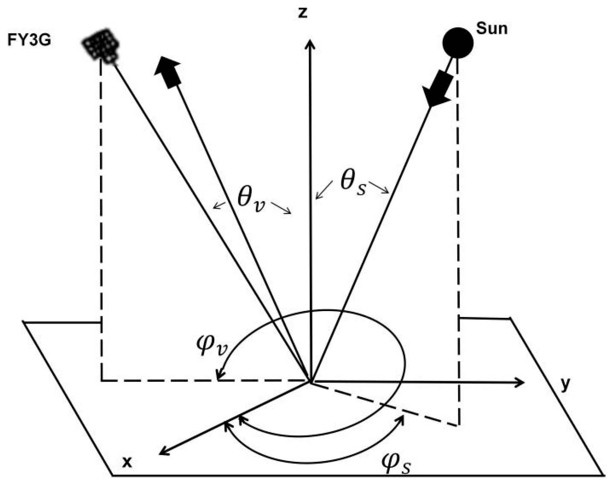
2.5. Sun Glint Geometry and Angle Definitions

Figure 1 presents a schematic illustration of the sun glint geometry and the corresponding angle definitions. The arrows indicate the incident direction of solar radiation and the reflected direction off the ocean surface, respectively. The symbol ${\theta }_s$ represents the solar zenith angle, which is the angle between the local pixel geodetic zenith and the solar direction. The symbol ${\phi }_s$ represents the solar azimuth angle, which is the clockwise angle from the local pixel geodetic north to the solar direction when viewed from above. The symbol ${\theta }_v$ represents the satellite zenith angle, which is the angle between the MWRI-RM line-of-sight vector and the zenith vector normal to the Earth’s ellipsoid. The symbol ${\phi }_v$ denotes the satellite azimuth angle, which is the clockwise angle from the local pixel geodetic north to the satellite’s direction when viewed from above. The sun glint angle ${\theta }_{glint}$ can be used as an indicator for identifying sun glint contamination. However, because of the absence of the sun glint flag in the MWRI-RM L1 data, the sun glint angle was calculated and defined by the following equation in this study [22]:

$${\theta }_{glint}=\arccos (\cos {\theta }_s\cos {\theta }_v-\sin {\theta }_s\sin {\theta }_v\cos |{\phi }_s-{\phi }_v|)$$

(2)

3. Results

3.1. Sun Glint Identification and Source Analysis

Figure 2 shows the spatial distributions of the model difference I, solar zenith angle ${\theta }_s$, and sun glint angle ${\theta }_{glint}$ at a horizontal polarized MWRI-RM channel of 10.65 GHz over the global ocean on 5, 11, 14, and 28 February 2024. The uncolored regions between adjacent orbital swaths in Figure 2 denote swath gaps. The uncolored areas within the swath represent land, coastlines, and sea ice regions, as well as detected cloudy and rainy pixels, as described in Section 2. As shown in Figure 2a, sun glint contamination can be effectively identified using the model regression difference method. The values of the model difference index I range from 0 K to 5 K. Warmer colors in the mapping indicate larger values of the model difference index I. On 5 February, the detected sun glint contamination was localized near the central portion of each swath on descending orbits. Contaminated pixels can be found in the mid-latitude band of the Northern Hemisphere from 10° N to 30° N. From 5 to 11 February, sun glint contamination in every scan line displaces eastward toward the swath’s right margin. During this period, it simultaneously shifts southward into the Southern Hemisphere. On 11 February, the contaminated pixels were observed in the equatorial zone between 0° S and 20° S. From 11 to 14 February, the detected contamination remains in a southward shift along the swath’s right margin toward the Southern Hemisphere. On 14 January, the contaminated pixels exhibiting a higher model difference index are identified near 20° S latitude and at the right-most position of each scanline. From 14 to 28 February, the contaminated FOVs continue to move southward. On 28 February, the contamination appears near the swath center on ascending orbits within 20° S to 30° S. Starting from 29 February, sun glint contamination begins to occur near the swath central region in all ascending orbits between 20° N and 50° N latitude. In contrast, no such contamination is identified in the descending mode.

The reason why contamination changes from the descending mode to the ascending mode is that MWRI-RM periodically reverses its flight direction, as described in Section 2.1. On 29 February, FY-3G conducted a 180° yaw maneuver to reverse the flight direction, so the contamination disappears from the Southern Hemisphere and occurs directly between the mid-latitudinal band of 30° N to 50° N. The spatial distributions and movement patterns of the contamination during the following 30-day cycle closely resemble the patterns illustrated in Figure 2a. The spatial distributions of sun glint contamination in the MWRI-RM 10.65 GHz channel at vertical polarization over oceanic surfaces exhibit similarities with those at horizontal polarization. However, the model difference index is slightly smaller than those at horizontal polarization, which is attributed to the lower ocean surface reflectivity at vertical polarization. The corresponding figures are omitted for brevity.

Figure 2b illustrates the spatial distributions of the solar zenith angle ${\theta }_s$ on 5, 11, 14, and 28 February 2024. It can be found that the high model difference values coincide with the solar zenith angle ${\theta }_s$ in the range of 45° to 60°, close to the instrument incidence angle. The MWRI-RM instrument performs conical scanning, maintaining a constant incident angle of 50°. As the solar zenith angle ${\theta }_s$ within FOVs is closer to 50°, the specular reflection direction of solar radiation approaches the incidence angle of MWRI-RM. This phenomenon results in the sun glint angle approaching 0°, enabling reflected solar radiation to enter the MWRI-RM antenna and contaminate measurements consequently. Because of its non-sun-synchronous orbital design, the FY-3G experiences daily variations in its geometry relative to the Sun. This dynamic relationship alters the solar zenith angle ${\theta }_s$ for fixed surface pixels over time. Consequently, the contaminated FOVs move back and forth between the latitudinal bands of the Northern and Southern Hemispheres along the scanning swath over a 30-day cycle.

Specular reflection mostly occurs over the ocean surfaces under low-wind conditions. Sun glint contamination in a microwave radiometer arises from the geometric relationship between two key directional parameters: the specular reflection angle of solar radiation off the ocean surface and the sensor’s incident angle. The occurrence of such contamination is determined by the angle proximity of these two vectors. Specifically, the sun glint angle ${\theta }_{glint}$, which quantifies the angular proximity between the two aforementioned vectors, serves as a critical indicator for detecting sun glint contamination. Figure 2c shows the spatial distributions of the sun glint angle ${\theta }_{glint}$ on 5, 11, 14, and 28 February 2024. A warmer color tone in Figure 2c corresponds to a smaller magnitude of the sun glint angle ${\theta }_{glint}$. A comparative analysis of Figure 2a,c demonstrates that contamination intensity and spatial distribution exhibit strong correspondence with the sun glint angle ${\theta }_{glint}$. Lower sun glint angles correlate with higher probabilities for the radiance measurements to be contaminated. Only FOVs with small sun glint angles are susceptible to the reflected solar radiation. Sun glint contamination is primarily concentrated in FOVs where the sun glint angle is below 10°. As the sun glint angle approaches 0°, the intensity of contamination increases correspondingly, meaning the closer the sun glint angle is to 0°, the stronger the contamination becomes.

3.2. Determination of the Sun Glint Flag Critical Angle

Given the absence of sun glint flags in MWRI-RM L1 data products, there is an urgent need to obtain a threshold angle for sun glint flagging. Figure 3 presents a 2-D histogram of the 10.65 GHz model differences versus sun glint angles for the contaminated observations collected between November 2023 and July 2024. The colorbar in Figure 3 indicates the occurrence of contaminated observations for each bin. The percentage is calculated over the total number of contaminated pixels. To prevent excessive counts from degrading the visual quality, the colorbar displays the percentage of contaminated observations for each bin rather than counts. The sun glint angle bins are characterized by a distance of 1°, while the model difference bins are characterized by 0.2 K. The data points included in this analysis were selected from every swath with model difference values in the 0–5 K range. The reasons for selecting data with positive index values are as follows: (a) Solar radiation reflected into the MWRI-RM antenna increases observed brightness temperatures, resulting in positive model difference values. (b) Larger positive values indicate a more significant sun glint impact on the observation accuracy, while negative values cannot stand for sun glint contamination. (c) Sun glint contamination is not denoted by negative values in the model simulation. As illustrated in Figure 3, a clear trend is evident: the model differences negatively correlate with the sun glint angles. A greater magnitude of the sun glint angle implies less probability of sun glint contamination. Specifically, when the sun glint angles range from 25° and 30°, the model difference values mostly fall within the 0–1 K range. Sun glint contamination occurs significantly less frequently compared to the circumstances of the sun glint angle between 0° and 25°. Additionally, in the lower sun glint angle bins, especially 0° and 10°, there are more observations with relatively higher model differences (up to 4–5 K).

Table 3. The monthly distribution of sun-glint-contaminated pixels for different sun glint angle intervals from November 2023 to July 2024 (unit: %).

Date	0° ≤ θglint ≤ 20°	20° < θglint ≤ 25°	25° < θglint ≤ 30°	θglint > 30°
Nov–Dec-2023	81.90 (3.06)	14.13 (0.52)	3.72 (0.14)	0.25 (0.01)
Jan–Feb-2024	82.89 (3.11)	13.18 (0.49)	3.80 (0.14)	0.13 (0.01)
Mar–Apr-2024	80.97 (3.05)	15.49 (0.58)	3.48 (0.13)	0.06 (0.00)
May–Jul-2024	84.75 (3.17)	12.09 (0.46)	3.11 (0.12)	0.05 (0.00)

presents the monthly distribution of sun-glint-contaminated pixels for different sun glint angle ${\theta }_{glint}$ intervals from November 2023 to July 2024. A statistical analysis of these contaminated pixels reveals that over 96% of the contaminated pixels observed between November 2023 and July 2024 have sun glint angles ${\theta }_{glint}$ ≤ 25°, with fewer than 4% of all the contaminated pixels featuring sun glint angles greater than 25°. Sun glint contamination was identified in only a small number of pixels when the sun glint angle exceeded 30°. The values in parentheses represent the percentage of contaminated pixels over the total number of observations, which shows that when the sun glint angle is below 25°, the percentage of contaminated pixels is less than 4%. This indicates a strong association between sun glint contamination and sun glint angles below 25°. This leads to the recommendation of 25° as the critical threshold angle for flagging sun glint in MWRI-RM 10.65 GHz observations.

3.3. Contamination at Other MWRI-RM Channels

Based on the method mentioned in Section 2, the spatial distributions of the model difference index I over the global ocean at the remaining MWRI-RM channels (ranging from 18.7 to 183.31 GHz) were also investigated. The MWRI-RM observations at these channels are not contaminated mainly because sun glint is most pronounced at 10 GHz. According to previous studies, the reasons are as follows: (a) the Sun has a higher brightness temperature at longer wavelengths, (b) the receiver has a better noise figure at lower frequencies, (c) the bandwidth of the channels is narrower at 10 GHz, (d) the ocean is more reflective at lower frequencies, and (e) there is less atmospheric attenuation at lower frequencies [20]. However, significant model difference values (exceeding 5 K) have been detected in the MWRI-RM 18.7 GHz channel. Tian indicated that the microwave radiometer measurements at 18.7 GHz over oceanic surfaces primarily experience contamination from geostationary television satellite downlink signals reflecting from the water [32]. Similar to RFI, this specific form of contamination is referred to as television frequency interference (TFI), arising from man-made active devices.

Figure 4 shows the spatial distributions of the index I (a) at the horizontal polarization of the MWRI-RM 18.7 GHz channel and the identification flag of radio frequency interference (b), which is RFI-Flag-recorded in the MWRI-RM L1 data, over the global ocean on 7 April 2024. The regression coefficients at 18.7 GHz have been given in Table 2. The training dataset utilized for establishing the simulation model of the 18.7 GHz channels is the same as that for the 10.65 GHz channels. Figure 4a shows the distinct highlighted color areas along the west coast of the United States. As mentioned above, these highlighted areas indicate the presence of TFI. The observed spatial–temporal patterns of TFI along the coastline of the U.S. are consistent with previous studies [33]. These studies reveal that intense TFI signals come from DirecTV satellites positioned near Hawaii and along the U.S. western and eastern coasts. Figure 4b shows the RFI-Flag in the MWRI-RM L1 data, which indicates a detection flag for radio frequency interference. RFI-Flag divides the pixel quality into two levels. A value of 0 means that the pixels are without RFI. A value of 1 means that the pixels are with RFI. As is shown in Figure 4b, there is no impact from RFI, and no TFI is detected, in contrast to the situation where TFI appears on the west coast of the United States in Figure 4a. Therefore, the model regression difference method effectively identifies TFI signals in regions where the RFI-Flag in MWRI-RM L1 data fails to detect them. Moreover, the sun glint contamination at 10.65 GHz is present in every orbit and moves regularly on a daily basis. The key characteristic of sun glint contamination is its spatial distribution related to solar geometry, specifically the sun glint angle. In contrast, pixels affected by TFI signals exhibit distinct temporal–spatial behaviors: they remain spatially stationary and temporally persistent, consistently appearing in regions illuminated by geostationary television satellite footprints. The distinct characteristics of TFI signals and sun glint contamination enable clear differentiation between their respective contaminated pixels. As described in previous studies, the TFI-free brightness temperature at 18.7 GHz channels can be predicted according to Equation (1) [32].

3.4. Validation and Statistical Evaluation for Sun Glint Correction

As described previously, sun glint only increases the brightness temperature of low-frequency channels. Therefore, the contaminated brightness temperature at low-frequency channels can be predicted using higher-frequency channels. To verify whether the model regression difference method can correct the contaminated brightness temperature, the observed brightness temperature of the 18.7 GHz horizontal polarization channel was selected as test data for correction. Figure 5 shows the spatial distributions of the observed brightness temperature (a), model-simulated brightness temperature (b), and the difference between the observed and simulated brightness temperatures (c) at the horizontal polarized MWRI-RM channel of 18.7 GHz on 10 February 2024. It can be seen that the simulated brightness temperature is highly consistent with the observed brightness temperature, with small discrepancies between them. Figure 5c shows that there are some pixels with large model differences (well above 5 K). Taking the selection of the training dataset into account, the difference values between the model simulations and observations may notably increase when the pixels are under specific rainy or cloudy conditions.

We further validated the effectiveness of the model regression difference method in reconstructing the brightness temperature. Figure 6a demonstrates a 2-D histogram of the observed brightness temperature versus the simulated brightness temperature at the horizontal polarized MWRI-RM channel of 18.7 GHz. The data included in the scatter plot within every swath were selected from November 2023 to July 2024 with model difference values [−5 K, 5 K] to avoid FOVs under rainy or cloudy conditions. The brightness temperature bins of the observations and simulations are both characterized by a distance of 1°. It is shown that a good agreement is obtained. The slope and intercept of the fitting line in Figure 6a are 1.0071 and 0.6923, with the mean bias (MB = 0.28) and root-mean-square error (RMSE = 0.39) quantitatively evaluating the agreement between the observations and simulations. Figure 6b presents the probability density distribution (PDF) of the difference between the observed and simulated brightness temperatures. The curve reveals the frequency of occurrence for different difference values, with a prominent peak near zero, indicating that most difference values are close to zero. In addition, the probability density for the model difference values within the [1 K, 5 K] range approaches zero, indicating that the occurrence frequency of the difference values in this interval is extremely low. This is likely due to the imperfect exclusion of pixels under rainy or cloudy conditions.

Next, a practical correction for sun glint on the 10.65 GHz horizontal polarization channel was conducted, where the contaminated brightness temperature was replaced by the simulated brightness temperature. After the brightness temperature contaminated by the sun glint in the 10.65 GHz channel was corrected, it was essential to validate the corrected brightness temperature. Although there are no true values for validation in brightness temperature observations, the high natural correlations between the MWRI-RM channels can be used as a verification indicator. Thus, the brightness temperature of the 18.7 GHz horizontal polarization channel was collected to assess whether the corrected brightness temperature of the 10.65 GHz horizontal polarization channel preserves the high natural correlations. Figure 7 shows the 2-D histogram of the observed brightness temperature at the 18.7 GHz channel versus the observed (a) and the simulated (b) brightness temperatures at the 10.65 GHz channel. The brightness temperature bins are both characterized by a distance of 1°. The rules for selecting the data are consistent with those of Figure 3, which contain sun glint contamination. As can be seen in Figure 7a, there are some abnormally high values in the brightness temperature observed at the MWRI-RM10.65 GHz channel. The correlation coefficient between the observed brightness temperature at the 18.7 GHz channel and the 10.65 GHz channel is 0.90. However, these abnormally high values disappeared after the correction process, as shown in Figure 7b. Moreover, the brightness temperature at the 10.65 GHz channel corrected by the model difference method has a relatively higher correlation with the observed brightness temperature at the 18.7 GHz channel. The correlation coefficient between the observed brightness temperature at the 18.7 GHz channel and the simulated brightness temperature at the 10.65 GHz channel is 0.98. Thus, the MWRI-RM contaminated brightness temperature can be corrected through the application of the multichannel regression technique.

4. Discussion

4.1. Advantages

The model regression difference method effectively identifies sun glint contamination in MWRI-RM measurements, offering several advantages. By using multichannel regression with the 18.7, 23.8, and 36.5 GHz channels, the method accurately simulates contamination-free brightness temperatures at 10.65 GHz. As shown in Figure 2, the sun glint contamination intensity (0–5 K increase in brightness temperature) correlates with sun glint angles ≤ 25°. The critical angle of the sun glint flags for MWRI-RM 10.65 GHz is 25°, validated through statistical analysis (Figure 3 and Table 3).

The method also detects TFI along U.S. coastlines, which RFI-Flag in Level 1 data fails to detect. As shown in Figure 4a, distinct spatial distributions of TFI contamination are observed in 18.7 GHz measurements along the U.S. west coast, coinciding with geostationary satellite signal coverage regions. In contrast, Figure 4b demonstrates that the RFI-Flag in MWRI-RM L1 data fails to identify these persistent signals, highlighting the method’s sensitivity. This dual capability to distinguish dynamic solar contamination (Figure 2) from static TFI signals (Figure 4) can improve data quality by enabling targeted correction.

The method can also correct the contaminated brightness temperature. As validated in Figure 7, the correction process removes abnormally high brightness temperatures in 10.65 GHz measurements. Specifically, the correlation coefficient between 10.65 GHz and 18.7 GHz observations increases from 0.90 (pre-correction) to 0.98 (post-correction), demonstrating restored natural channel relationships. This method, which can identify sun-glint- or TFI-contaminated pixels, correct contaminated data, and improve data accuracy, can be easily applied to other microwave radiometers aboard following low-inclination FengYun satellites. It relies on publicly available data and has a simple implementation process. This simplicity allows the approach to be adapted and scaled up for different satellite missions without requiring complex adjustments or specialized resources.

4.2. Limitations

While the model regression difference method proposed in this study demonstrates effective performance in detecting sun glint contamination, there are still some limitations in this method. First, the reliance on clear-sky training data introduces uncertainty to regions with persistent cloud cover, potentially degrading model accuracy. While Figure 5 and Figure 6 show small difference values between simulated and observed brightness temperatures at 18.7 GHz (0–1 K), large values under complex atmospheric conditions (e.g., rain/cloud) suggest a need for improved cloud masking algorithms. Second, the critical angle of 25° is validated for 10.65 GHz and MWRI-RM, but extrapolation to other sensors requires independent verification.

Additionally, the method’s effectiveness in high-wind conditions, which differ from specular reflection, remains untested. Figure 5 highlights large model differences (>5 K) in 18.7 GHz channels, indicating potential limitations in training dataset selection. The absence of ground-truth data limits accuracy assessment. To address these limitations, future work should use radiative transfer models, expand validation with in situ measurements taken into consideration, and refine training datasets to encompass diverse atmospheric conditions.

5. Conclusions

Evaluating the accuracy of space-borne passive microwave radiometer measurements is critical for geophysical parameter retrieval. Contaminated observations, such as those affected by sun glint or radio frequency interference, must be identified and corrected. This study employs FY-3G/MWRI-RM as a case study, utilizing the model regression difference method to compute the differences between observed and model-simulated brightness temperatures. This approach enables the detection of sun glint contamination in global oceanic regions at MWRI-RM low-frequency channels. A detailed analysis is conducted on the intensity of biases in brightness temperature caused by sun glint and the critical angle for flagging contaminated observations. Moreover, brightness temperature contaminated by sun glint can be effectively corrected by the multichannel regression technique. The primary findings are summarized as follows:

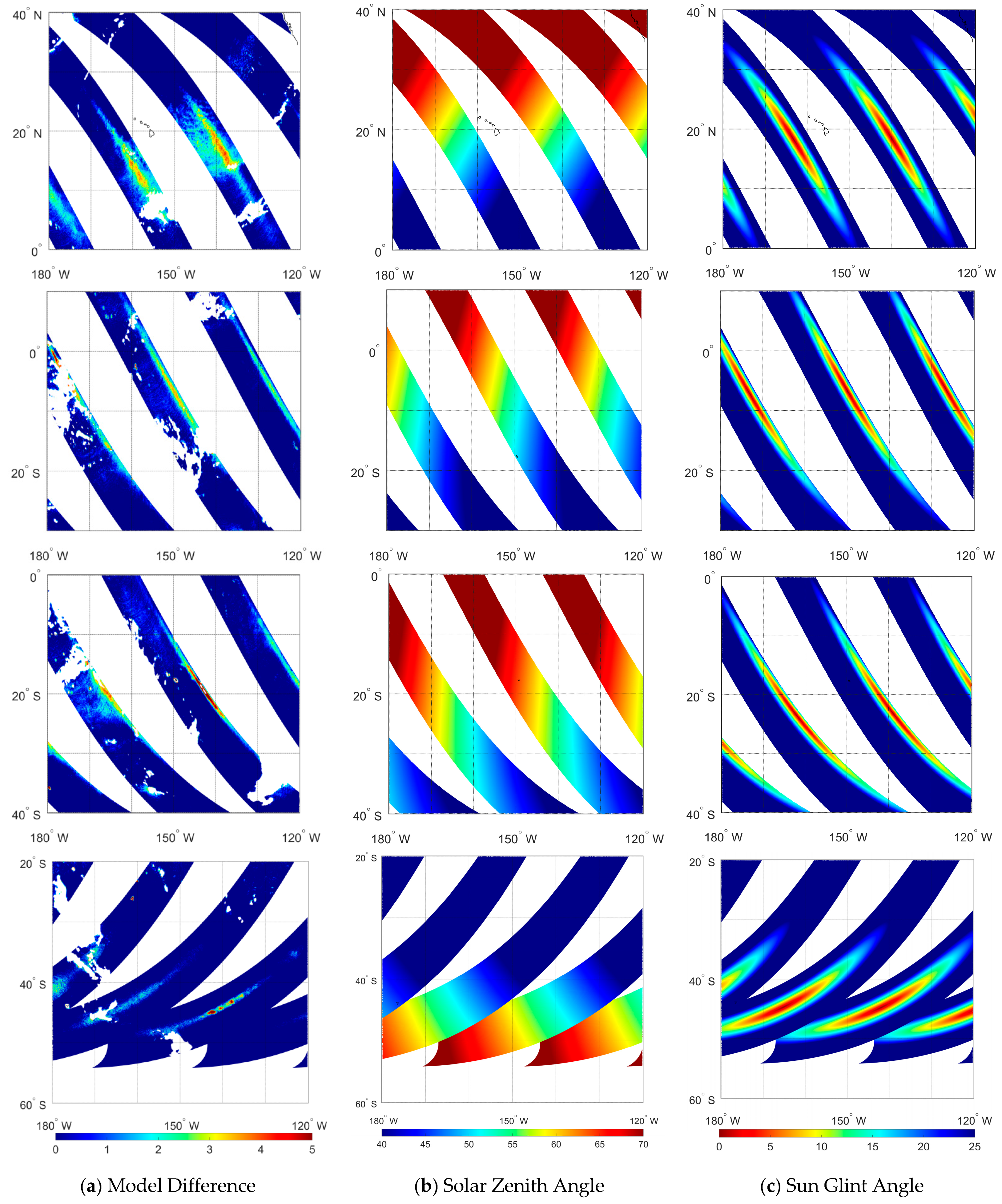
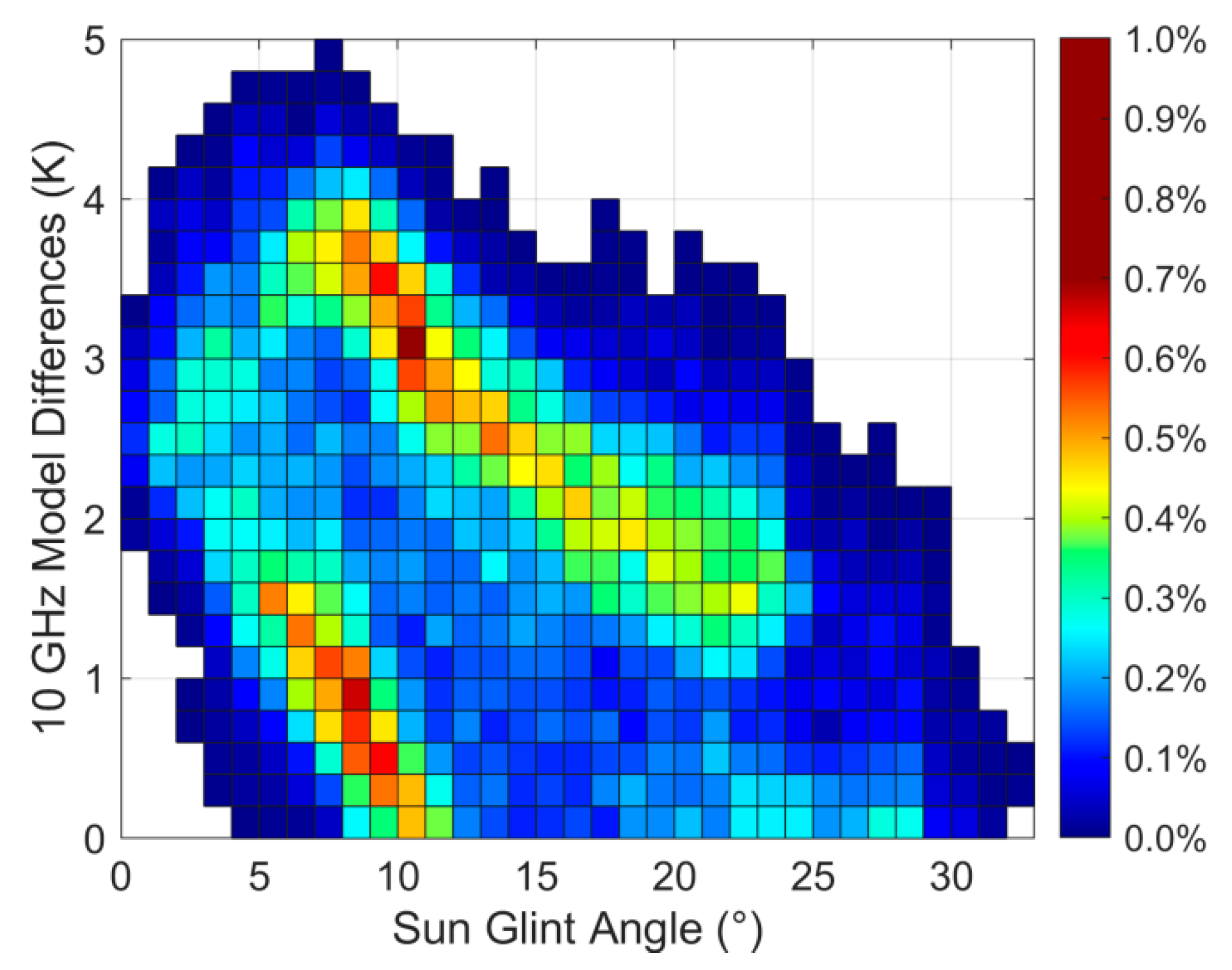
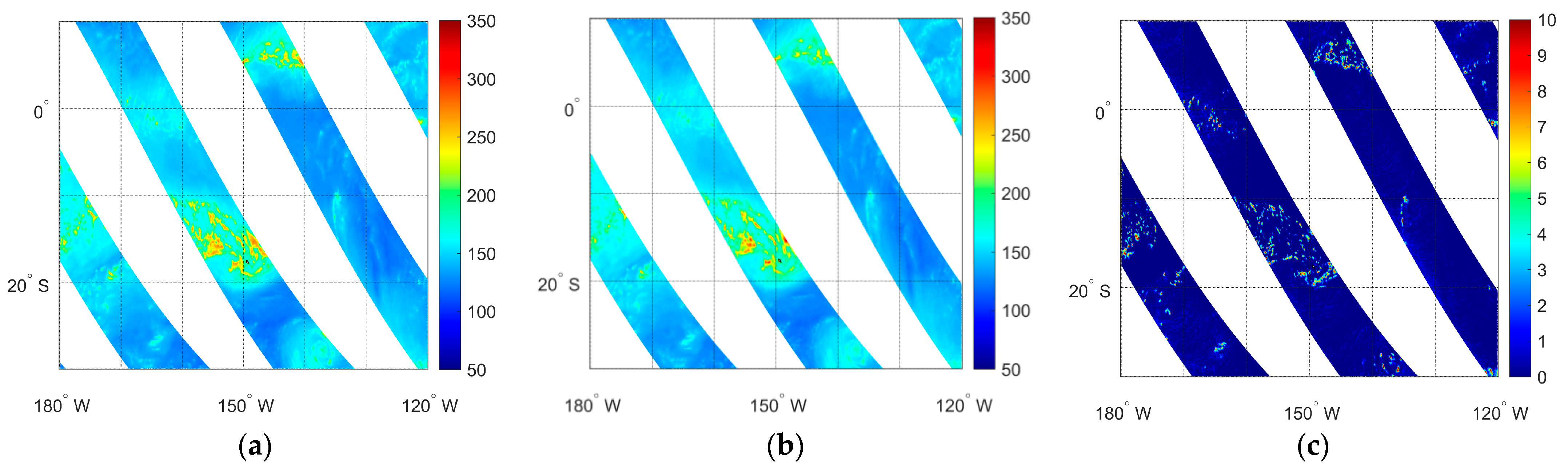
• Observations over the global ocean at the MWRI-RM 10.65 GHz channel are occasionally affected by specular reflection of solar radiation from the ocean surface. The intensity and locations of the contamination exhibit a strong correlation with the value of the sun glint angle. The closer the sun glint angle is to 0°, the stronger the contamination is. The increment in observed brightness temperatures due to reflected solar radiation falls within the range of [0 K, 5 K]. The range of the solar zenith angle associated with large model difference values falls within [45°, 60°].
• Through a detailed quantitative analysis of sun glint angle distributions in the contaminated pixels, the statistical results reveal that over 96% of such pixels have sun glint angles ≤ 25°, with fewer than 4% exceeding 25°. This strong correlation between contaminated pixels and angles below 25° justifies recommending 25° as the critical threshold for sun glint flagging in MWRI-RM 10.65 GHz observations.
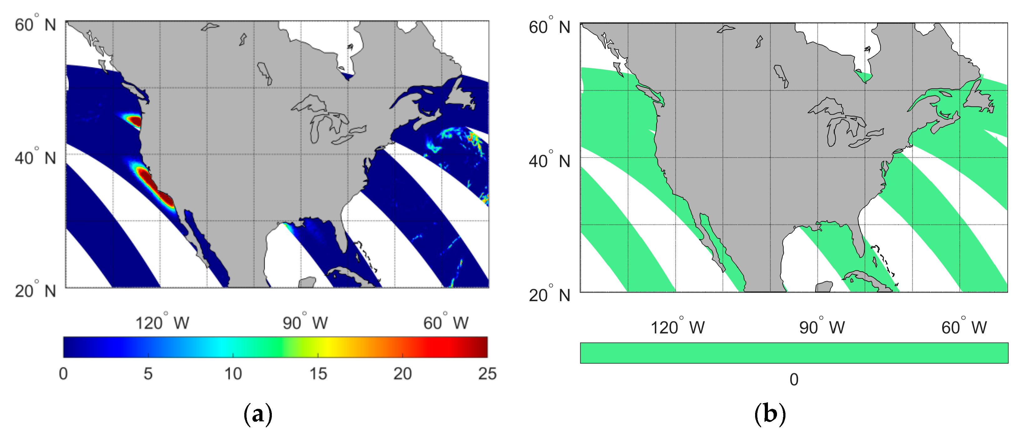
• The TFI along the U.S. coastline can be effectively detected using the model regression difference method, as demonstrated in the analysis of MWRI-RM Level 1 data, where the standard RFI-Flag product failed to identify these persistent interference signals. The spatial distribution of TFI signals differs significantly from that of sun glint contamination.
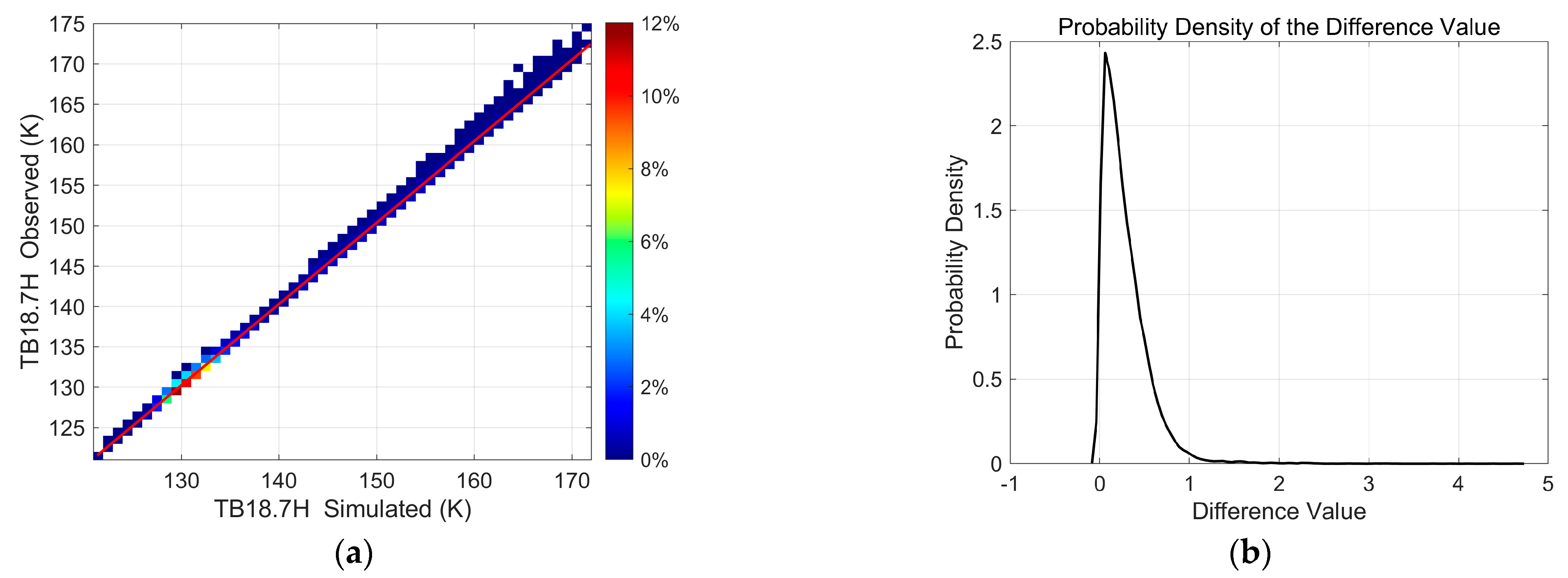
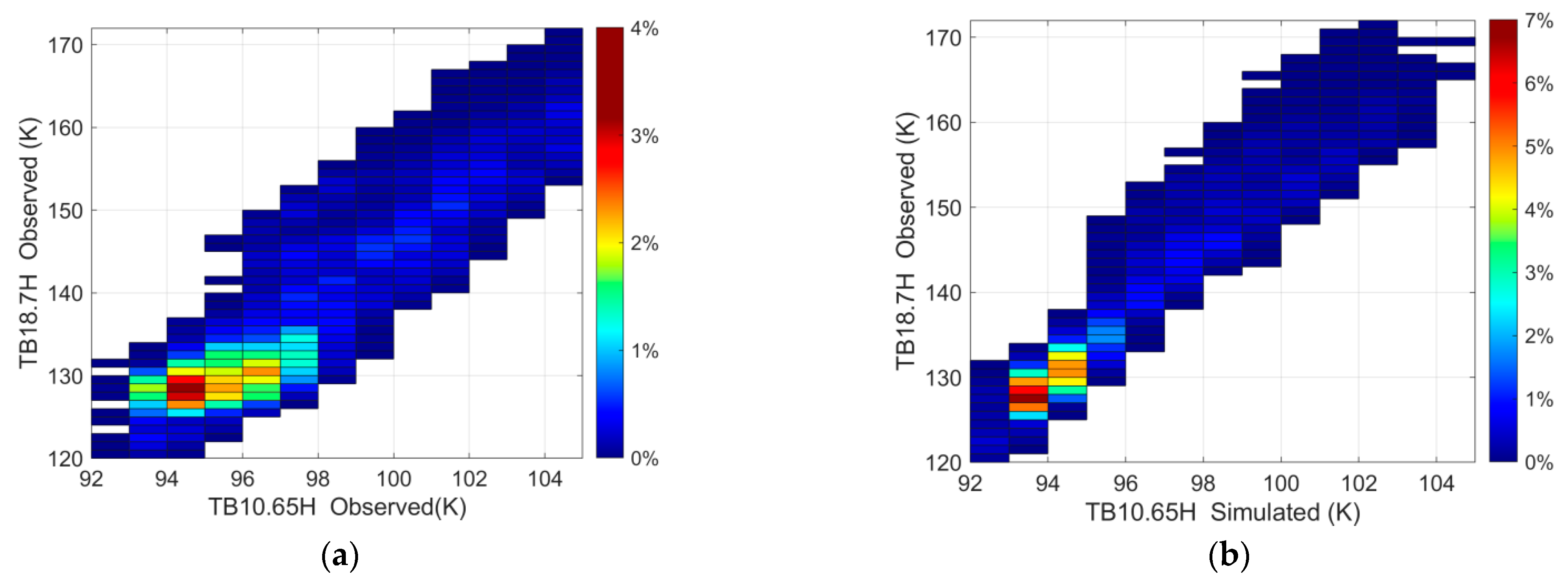
• The MWRI-RM brightness temperature at 10.65 GHz contaminated by sun glint can be corrected by the multichannel regression technique, which is validated by improved correlation (from 0.90 to 0.98) with the 18.7 GHz channel.

References

1. Hollinger, J.P.; Peirce, J.L.; Poe, G.A. SSM/I instrument evaluation. IEEE Trans. Geosci. Remote Sens. 1990, 28, 781–790. [Google Scholar] [CrossRef]
2. Kummerow, C.; Barnes, W.; Kozu, T.; Shiue, J.; Simpson, J. The tropical rainfall measuring mission (TRMM) sensor package. J. Atmos. Ocean. T. 1998, 15, 809–817. [Google Scholar] [CrossRef]
3. Kawanishi, T.; Sezai, T.; Ito, Y.; Imaoka, K.; Takeshima, T. The advanced microwave scanning radiometer for the earth observing system (AMSR-E), NASDA’s contribution to the EOS for global energy and water cycle studies. IEEE Trans. Geosci. Remote Sens. 2003, 41, 184–194. [Google Scholar] [CrossRef]
4. Gaiser, P.W.; St Germain, K.M.; Twarog, E.M.; Poe, G.A.; Purdy, W. The Wind Satspaceborne Polarimetric microwave radiometer: Sensor description and early orbit performance. IEEE Trans. Geosci. Remote Sens. 2004, 42, 2347–2361. [Google Scholar] [CrossRef]
5. Spencer, R.W.; Christy, J.R.; Braswell, W.D. UAH Version 6 global satellite temperature products: Methodology and results. Asia-Pac. J. Atmos. Sci. 2017, 53, 121–130. [Google Scholar] [CrossRef]
6. Draper, D.; Newell, D.; Wentz, F.; Krimchansky, S.; Skofronick-Jackson, G. The Global Precipitation Measurement (GPM) Microwave Imager (GMI): Instrument Overview and Early On-Orbit Performance. IEEE Trans. Geosci. Remote Sens. 2015, 8, 3452–3462. [Google Scholar] [CrossRef]
7. Xia, X.; He, W.Y.; Wu, S.L. A thorough evaluation of the passive microwave radiometer measurements onboard three Fengyun-3 satellites. J. Meteorol. Res. 2023, 37, 573–588. [Google Scholar] [CrossRef]
8. Varotsos, C.A.; Krapivin, V.F.; Mkrtchyan, F.A. A New Passive Microwave Tool for Operational Forest Fires Detection: A Case Study of Siberia in 2019. Remote Sens. 2020, 12, 835. [Google Scholar] [CrossRef]
9. Nazari-Sharabian, M.; Aghababaei, M.; Karakouzian, M.; Karami, M. Water on Mars—A Literature Review. Galaxies 2020, 8, 40. [Google Scholar] [CrossRef]
10. Cho, J.; Lee, Y.W.; Lee, H.S. Assessment of the relationship between thermal-infrared-based temperature-vegetation dryness index and microwave satellite-derived soil moisture. Remote Sens. Lett. 2014, 5, 627–636. [Google Scholar] [CrossRef]
11. Shi, Z.; Zou, X. Diurnal variations of radio-frequency interference signal detected from FY-3G Microwave Radiation Imager-Rainfall Mission. J. Meteorol. Sci. 2024, 44, 691–706. [Google Scholar]
12. Zou, X.; Zhao, J.; Weng, F.; Qin, Z. Detection of radio-frequency interference signal over land from FY-3B Microwave Radiation Imager (MWRI). IEEE Trans. Geosci. Remote Sens. 2012, 50, 4994–5003. [Google Scholar] [CrossRef]
13. Zhao, J.; Zou, X.; Weng, F.Z. WindSat radio-frequency interference signature and its identification over Greenland and Antarctic. IEEE Trans. Geosci. Remote Sens. 2013, 51, 4830–4839. [Google Scholar] [CrossRef]
14. Martin-Porqueras, F.; Floury, N.; Martin-Neira, M. Detection of the L-band Galactic Glint on the sea surface with the airborne MIRAS. IEEE Trans. Geosci. Remote Sens. 2010, 48, 1968–1975. [Google Scholar] [CrossRef]
15. Kunkee, D.B.; Swadley, S.D.; Poe, G.A.; Hong, Y.; Werner, M.F. Special Sensor Microwave Imager Sounder (SSMIS) Radiometric Calibration Anomalies-Part I: Identification and Characterization. IEEE Trans. Geosci. Remote Sens. 2008, 46, 1017–1033. [Google Scholar] [CrossRef]
16. Wentz, F.; Ashcroft, P.; Gentemann, C. Post-launch calibration of the TRMM Microwave Imager. IEEE Trans. Geosci. Remote Sens. 2001, 39, 415–422. [Google Scholar] [CrossRef]
17. Geer, A.J.; Bauer, P.; Bormann, N. Solar Biases in Microwave Imager Observations Assimilated at ECMWF. IEEE Trans. Geosci. Remote Sens. 2010, 48, 2660–2669. [Google Scholar] [CrossRef]
18. Tropical Rainfall Measuring Mission Precipitation Processing System File Specification 2A12; Version 7; NASA-GSFC: Greenbelt, MD, USA, 2013; pp. 15–16.
19. GMI Calibration Algorithm and Analysis Theoretical Basis Document; Remote Sensing Systems: Santa Rosa, CA, USA, 2011; pp. 87–90.
20. Xue, Q.M.; Guan, L. Identification of Sun Glint Contamination in GMI Measurements Over the Global Ocean. IEEE Trans. Geosci. Remote Sens. 2019, 57, 6473–6483. [Google Scholar] [CrossRef]
21. Remer, L.A.; Kaufman, Y.J.; Tanré, D. The MODIS Aerosol Algorithm, Products, and Validation. J. Atmos. Sci. 2005, 62, 947–973. [Google Scholar] [CrossRef]
22. Chen, Z.T.; Sun, X.B.; Wang, J.F. Dynamic detection of ocean glint from near-infrared polarized radiation satellite data. J. Remote Sens. 2019, 23, 215–229. [Google Scholar] [CrossRef]
23. Cox, C.; Munk, W. Measurements of the roughness of the sea surface from photographs of the sun’s glitter. J. Opt. Soc. Am. 1964, 44, 838–850. [Google Scholar] [CrossRef]
24. Cox, C.; Munk, W. Statistics of the sea surface derived from sun glitter. J. Mar. Res. 1954, 13, 198–227. [Google Scholar]
25. Ebuchi, N.; Kizu, S. Probability distribution of surface wave slope derived using sun glitter images from geostationary meteorological satellite and surface vector winds from scatterometers. J. Oceanogr. 2002, 58, 477–486. [Google Scholar] [CrossRef]
26. Bréon, F.M.; Henriot, N. Spaceborne observations of ocean glint reflectance and modeling of wave slope distributions. J. Geophys. Res. Ocean. 2006, 111, C06005. [Google Scholar] [CrossRef]
27. Kay, S.; Hedley, J.D.; Lavender, S. Sun glint correction of high and low spatial resolution images of aquatic scenes: A review of methods for visible and near-infrared wavelengths. Remote Sens. 2009, 1, 697–730. [Google Scholar] [CrossRef]
28. Zhang, P.; Gu, S.; Chen, L.; Shang, J.; Lin, M.; Zhu, A.; Yin, H.; Wu, Q.; Shou, Y.; Sun, F.; et al. FY-3G satellite instruments and precipitation products: First report of China’s Fengyun rainfall mission in-orbit. J. Remote Sens. 2023, 3, 0097. [Google Scholar] [CrossRef]
29. Li, L.; Gaiser, P.W.; Bettenhausen, M.H. WindSat radio-frequency interference signature and its identification over land and ocean. IEEE Trans. Geosci. Remote Sens. 2006, 44, 530–539. [Google Scholar] [CrossRef]
30. Draper, D.W. Terrestrial and space-based RFI observed by the GPM microwave imager (GMI) within NTIA semi-protected passive earth exploration bands at 10.65 and 18.7 GHz. In Proceedings of the 2016 Radio Frequency Interference, Socorro, NM, USA, 17–20 October 2016. [Google Scholar]
31. Grody, N. Classification of snow cover and precipitation using the special sensor microwave imager. J. Geophys. Res. Atmos. 1991, 96, 7423–7435. [Google Scholar] [CrossRef]
32. Tian, X.; Zou, X. An Empirical Model for Television Frequency Interference Correction of AMSR2 Data Over Ocean Near the U.S. and Europe. IEEE Trans. Geosci. Remote Sens. 2016, 54, 3856–3867. [Google Scholar] [CrossRef]
33. Draper, D.W.; Stocker, E.F. A comparison of radio frequency interference within and outside of allocated passive earth exploration bands at 10.65 GHz and 18.7 GHz using the GPM microwave imager and WindSat. In Proceedings of the 2017 IEEE International Geoscience and Remote Sensing Symposium, Fort Worth, TX, USA, 23–28 July 2017. [Google Scholar]
Figure 1. The schematic illustration of the sun glint geometry and the corresponding angle definitions.
Atmosphere 16 00630 g001
Figure 2. The global oceanic distribution patterns of the model difference index I (a), solar zenith angle (b), and sun glint angle (c) at the horizontal polarized MWRI-RM channel of 10.65 GHz on 5 (line 1), 11 (line 2), 14 (line 3), and 28 (line 4) February 2024.
Atmosphere 16 00630 g002
Figure 3. A 2-D histogram of 10.65 GHz model differences versus sun glint angles for contaminated observations.
Atmosphere 16 00630 g003
Figure 4. The spatial distributions of the model difference index at the horizontal polarization of the MWRI-RM 18.7 GHz channel (a) and the RFI-Flag recorded in the MWRI-RM L1 data (b) over the global ocean on 7 April 2024.
Atmosphere 16 00630 g004
Figure 5. The spatial distributions of the observed brightness temperature (a), model-simulated brightness temperature (b), and the difference between observed and simulated brightness temperature (c) at the horizontal polarized MWRI-RM channel of 18.7 GHz over the global ocean on 10 February 2024.
Atmosphere 16 00630 g005
Figure 6. A 2-D histogram of the observed brightness temperature versus the simulated brightness temperature at the horizontal polarized MWRI-RM channel of 18.7 GHz (a) and the probability density distribution (PDF) of the difference between the observed brightness temperature and the simulated brightness temperature (b).
Atmosphere 16 00630 g006
Figure 7. A 2-D histogram of the observed brightness temperature at the 18.7 GHz channel versus the observed (a) and the simulated (b) brightness temperatures at the 10.65 GHz channel.
Atmosphere 16 00630 g007