Abstract
Accurate estimation of anthropogenic CO2 emissions is crucial for effective climate change mitigation policies. This study aims to improve CO2 emission estimates in China using remote sensing measurements of column-averaged dry air mole fractions of CO2 (XCO2) and a neural network approach. We evaluated XCO2 anomalies derived from three background XCO2 concentration approaches: CHN (national median), LAT (10-degree latitudinal median), and NE (N-nearest non-emission grids average). We then applied the Generalized Regression Neural Network model, combined with a partition modeling strategy using the K-means clustering algorithm, to estimate CO2 emissions based on XCO2 anomalies, net primary productivity, and population data. The results indicate that the NE method either outperformed or was at least comparable to the LAT method, while the CHN method performed the worst. The partition modeling strategy and inclusion of population data effectively improved CO2 emission estimates. Specifically, increasing the number of partitions from 1 to 30 using the NE method resulted in mean absolute error (MAE) values decreasing from 0.254 to 0.122 gC/m2/day, while incorporating population data led to a decrease in MAE values between 0.036 and 0.269 gC/m2/day for different partitions. The present methods and findings offer critical insights for supporting government policy-making and target-setting.
1. Introduction
Global climate warming is advancing at an unprecedented rate, primarily driven by greenhouse gas (GHG) emissions. The warming has led to glacier melting, the sea surface rising, coral death, and extreme weather events across the globe [1,2,3]. To control GHG emissions and alleviate the impacts of climate change, many countries have taken action following the adoption of the Paris Agreement by 196 Parties in 2015. China, for instance, has committed to reaching a carbon peak by 2030 and carbon neutrality by 2060 [4]. Carbon dioxide (CO2), one of the primary GHGs, is the main driver of global warming, contributing to 70% of the greenhouse effect [5,6]. Therefore, accurate estimation of CO2 emissions is crucial, as it underpins the setting of targets and the formulation of policies. Moreover, it provides a better understanding of the carbon cycle and future climate projections [7,8].
Two major approaches have been applied to estimate anthropogenic CO2 emissions: bottom–up and top–down approaches. The bottom–up method relies on energy consumption statistics and emission factors. However, it is hampered by various issues, such as incomplete energy statistics, uncertainties in emission factors, and inconsistencies in data quality across regions [9,10]. In contrast, the top–down method uses satellite observation technologies, providing an alternative approach for estimating CO2 emissions. Satellites, such as the Greenhouse Gases Observing Satellite (GOSAT) [11], GOSAT-2, the Orbiting Carbon Observatory-2 (OCO-2) [12,13], OCO-3, and TanSat [14], have provided measurements of column-averaged dry air mole fractions of CO2 (XCO2), thereby enabling the global observation of atmospheric CO2 concentrations. Several studies have demonstrated that the spaceborne XCO2 data can reflect changes in atmospheric CO2 concentrations due to anthropogenic CO2 emissions. The signal of human activities, referred to as the “XCO2 anomaly”, can be detected by removing the background XCO2 concentration from the XCO2 observations, a process known as “XCO2 enhancement”. Kort et al. [15] employed GOSAT observations from nearby background regions (e.g., basins and deserts) and observed XCO2 enhancements of 3.2 1.5 ppm for Los Angeles, USA, and 2.4 1.2 ppm for Mumbai, India. Schwandner et al. [16] observed XCO2 enhancement ranging from 4.1 to 6.1 ppm over the Los Angeles urban area using OCO-2 data. Hakkarainen et al. [17] demonstrated a positive correlation between CO2 anomalies and emission inventories. Despite these advancements, extracting the anthropogenic CO2 emission signal remains challenging, because the signal is much smaller than the atmospheric CO2 concentration and is influenced by the inter-annual variability and transportation of atmospheric CO2 [9,17,18]. Inaccurate determination of background XCO2 concentrations will lead to significant errors in CO2 emission inversion [19,20].
Previous studies have proposed three main categories of methods to derive the background XCO2 concentration. The first category is to use the median or average within the selected region or latitudinal band. This method neglects the atmospheric transport process and deduces the background XCO2 concentration based only on the median or average value across the study area, as seen in numerous studies [17,21,22]. The second category is the regional comparison method. Here, the “clean areas”, or regions unaffected by anthropogenic CO2 emissions, are chosen as the XCO2 background area. The mean value over these regions is defined as the background XCO2 concentration [6,23,24]. The third category is the trajectory–endpoint method, which uses an atmospheric transport model to identify regions that are not influenced by CO2 emissions, and the mean XCO2 value over those regions is defined as the background concentration [20]. The identification of background XCO2 concentration has evident impacts on XCO2 enhancement and further influences CO2 emission inversion. However, only a few studies have evaluated the characteristics of these methods in defining background XCO2 concentration [25].
Several machine learning methods have been applied to estimate anthropogenic CO2 emissions from XCO2 anomalies. For example, Yang et al. [21] introduced the General Regression Neural Network (GRNN) model to estimate anthropogenic CO2 emissions from GOSAT data, demonstrating its ability to capture the nonlinear relationship between XCO2 anomalies and ODIAC data. Mustafa et al. [22] enhanced the GRNN model by incorporating the net primary productivity (NPP) data as an input, thereby accounting for the influence of CO2 uptake. Zhang et al. [26] developed a two-layer stacked random forest regression model to estimate anthropogenic CO2 emissions at the grid scale, with specific attention paid to variable selection. Their model used the XCO2 anomalies, the night-time light, the ecosystem respiration, the solar-induced chlorophyll fluorescence, and the enhanced vegetation index as driving variables. Ji et al. [27] proposed three machine learning algorithms—LightGBM, XGBoost, and CatBoost—to predict anthropogenic CO2 emissions with clustering of the CO2 concentration. Zhang et al. [28] employed the XGBoost model to explore the complex drivers of CO2 emissions in megacities. Uyar et al. [29] utilized four algorithms—gradient boosting trees (GBTs), random forest (RF), support vector machines (SVMs), and classification and regression trees (CARTs)—to estimate carbon emissions based on multiple environmental parameters. Other machine learning approaches, such as artificial neural networks (ANNs) and long short-term memory (LSTM) models, have also been applied to estimate daily CO2 emissions [30]. However, these models face challenges in accurately modeling anthropogenic CO2 emissions due to the high heterogeneity and non-normal distribution features of CO2 emissions, which are closely linked to human activities. Since significant human activities are mainly concentrated in urban areas, cities account for 70% of global energy-related carbon emissions [31]. These features must be fully recognized to achieve accurate model simulations.
In the present study, we addressed the challenges in extracting background XCO2 concentration and modeling spatial–heterogeneous CO2 emissions, focusing on mainland China as the study area. First, we derived the background XCO2 concentration using three approaches: the median XCO2 value across all grids within China (CHN method), the median within 10-degree latitudinal bands (LAT method), and the average XCO2 value from the N-nearest non-emission grids (NE method). We applied these methods to OCO-2 GEOS L3 data and evaluated their characteristics in XCO2 enhancement. Then, we proposed a CO2 emissions estimation method based on K-means clustering and the GRNN model, using XCO2 anomalies, net primary productivity (NPP), and population data as inputs and the Open-source Data Inventory for Anthropogenic CO2 (ODIAC) data as output. The model was calibrated using data from 2015 to 2020, with validation performed on data from 2021. The methods and findings of this study will enhance our understanding of XCO2 enhancement and provide effective methodologies for improving anthropogenic CO2 emissions estimation based on remote sensing.
2. Materials and Methods
2.1. Datasets
2.1.1. Column-Averaged Dry Air Mole Fraction of CO2 (XCO2)
The column-averaged dry air mole fraction of CO2 (XCO2) represents the column concentration of carbon dioxide observed by the carbon satellite. In this study, we used the OCO-2 GEOS L3 data [32] for XCO2 enhancement. The dataset was generated using data assimilation techniques, which integrate model simulations and OCO-2 satellite observations. We used the OCO-2 GEOS Level 3 data from 2015 to 2021, which have a spatial resolution of 0.5° × 0.625°. During this time, XCO2 values in China increased from 398.597–402.793 ppm in 2015 to 414.101–418.619 ppm in 2021 (Figure S1). To feed into the CO2 emission inversion model, we resampled the data to a spatial resolution of 1° × 1° using the bilinear interpolation method.
2.1.2. Net Primary Productivity (NPP)
The net primary productivity (NPP) represents the amount of organic carbon that plants fix through photosynthesis minus the carbon they expend during respiration. A positive NPP value indicates the absorption of atmospheric CO2, while a negative value indicates a release. Due to the processes of photosynthesis and respiration, vegetation activities directly regulate the process of the carbon cycle, influencing the atmospheric CO2 concentration. Thus, in this study, we utilized the global annual NPP dataset (MOD17A3HGF Version 6.1), generated by the Moderate Resolution Imaging Spectroradiometer (MODIS) [33], to represent the influence of vegetation activities. This dataset, available at a 15-arcsecond resolution, spans from 2001 to the present. The NPP values ranged from 74.628 to 15,920.204 kgC/m2/year averaged over 2015–2021 for China. To feed into our model, we aggregated the dataset to a 1° × 1° resolution using mean values.
2.1.3. Population
Anthropogenic CO2 emissions are highly related to human activities, as presented in Figure S2. Given that the heterogeneous distribution of population contributes to the non-normal distribution of CO2 emissions, we applied the LandScan Global population dataset as model input. LandScan Global [34] is a global annual population dataset with a 30-arcsecond resolution, representing the ambient (24-h average) population from 2000 to the present. Each cell in this dataset indicates the estimated population count. For our model, we aggregated this dataset to a 1° × 1° resolution by summing the values.
2.1.4. Fossil Fuel CO2 Emissions
For the fossil fuel CO2 emissions dataset, we utilized the Open-source Data Inventory for Anthropogenic CO2 (ODIAC) dataset [35]. This dataset provides a global gridded CO2 emission inventory of fossil fuel combustion based on satellite-based night-time light and individual power plant emissions. It is available at resolutions of 1 km × 1 km and 1° × 1°, effectively representing the spatiotemporal distribution of anthropogenic CO2 emissions. We utilized the 2022 version of the dataset, with a resolution of 1° × 1° covering the period from 2000 to 2021. In China, fossil fuel CO2 emissions ranged from 0 to 19.911 gC/m2/day in 2015, increasing to 0 to 23.200 gC/m2/day in 2021 (Figure S1). It is noted that the unit for fossil fuel CO2 emissions is grams of carbon per square meter per day (gC/m2/day), and all CO2 emission data in this study are reported based on the mass of carbon rather than carbon dioxide, consistent with the units used in the ODIAC dataset. For use as the model’s dependent variable, the monthly data were averaged to an annual scale.
2.2. Methods
We estimated anthropogenic CO2 emissions through a four-step procedure, as illustrated in Figure 1. First, we applied three methods for defining the background XCO2 concentration and then derived the XCO2 anomalies. Next, for the convenience of modeling the high heterogeneity and non-normal distribution features, we divided the study area into several partitions with the K-means clustering algorithm, based on the NPP and the ODIAC datasets. Then, we established a Generalized Regression Neural Network (GRNN) model for each partition, using annual XCO2 anomalies, NPP, and population data from 2015 to 2020 as inputs, with the ODIAC data for the same period serving as output. Finally, we validated the model by comparing the estimated CO2 emissions against the ODIAC data for 2021. All procedures were implemented in Python 3.9.17 (Python Software Foundation, Wilmington, DE, USA), with model execution parallelized using Pytorch 1.13.1 (Meta Platforms Inc., Menlo Park, CA, USA). The following sections provide a detailed explanation of each of these steps.
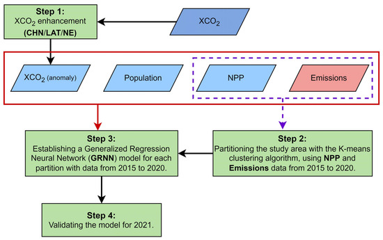
Figure 1.
A flowchart of the methodology adopted in the present study.
2.2.1. XCO2 Enhancement
The initial step in estimating CO2 emissions is to distinguish the concentration changes specifically attributable to CO2 emissions. We derived the XCO2 anomaly by subtracting the daily XCO2 background concentration from individual XCO2 measurements, following the method proposed by Hakkarainen et al. [17], as follows:
This equation enables the deseasonalization and detrending of the data, as and are retrieved simultaneously from geographically proximate regions or latitudes, which are expected to share similar seasonal patterns and long-term trends [17]. The definition of is critical for determining XCO2 enhancement. Previous studies have proposed several methods for deriving , typically using the median or mean value of XCO2 observations within the background region [17,22,36,37]. In terms of defining the background region, some studies have used the entire study area as a single background region, while others have applied each 10-degree latitudinal band [38,39]. Additionally, some studies have incorporated potential temperature and non-emission areas to define the background region [23]. In the present study, we applied three methods (illustrated in Figure 2) to derive and further assessed their effectiveness in estimating CO2 emissions.
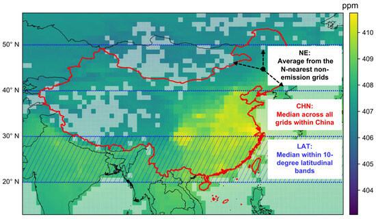
Figure 2.
A schematic diagram illustrating the three methods used in this study for deriving the background XCO2 concentration. The background color indicates the average XCO2 distribution from 2015 to 2021. The white transparent grids represent non-emission areas.
- (i)
- CHN method
For the CHN method, we defined the entire area of China as the background region and adopted the median XCO2 value within China as the background value, following the approach used by Hakkarainen et al. [17]. This approach assigns the same background value to all grids within China for each time step.
- (ii)
- LAT method
The LAT method divides China into several zones based on 10-degree latitudinal bands. The median XCO2 value of all grids within each latitudinal band is taken as the for that band, following the method proposed by Hakkarainen et al. [39]. To avoid abrupt changes near the boundaries of each latitudinal band, we linearly interpolated the background values according to latitude. Readers are directed to Hakkarainen et al. [39] for more details.
- (iii)
- NE method
Wang et al. [23] proposed a method to derive the background XCO2 concentration based on the ODIAC dataset and potential temperature data. In the present study, we followed the idea of zoning and regional comparison and simplified the method of Wang et al. [23] by relying solely on the ODIAC data. This approach, referred to as the NE method in the present study, identifies grids with zero CO2 emissions in the ODIAC dataset as non-emission regions. For each grid, the N-nearest non-emission grids were selected as the background region, and the average XCO2 value over these non-emission grids was used as the background value for that grid. We evaluated the performance with 5, 10, and 15-nearest non-emission grids and found minimal differences among these approaches (Figure S3). To ensure stability while reducing complexity, we applied the 10-nearest non-emission grids for the NE method throughout this study.
We first derived the daily with these three methods. We then calculated by subtracting the from the of each grid for each time step, as presented in Equation (1). We subsequently averaged within each grid for each year to obtain the annual average .
2.2.2. Estimating Emissions with GRNN Model
To represent the nonlinear relationship between CO2 emissions and the independent variables, i.e., XCO2 anomalies, NPP, and population data, we applied the GRNN algorithm [40] as the fundamental model. As a nonparametric regression, the GRNN model is designed and trained based on all known samples, with only one smoothing parameter. Moreover, the estimation results can be reproduced reduplicatively, since there are no random variables in the GRNN model. These characteristics of the GRNN model have led to its wide use in studies similar to the present one [21,22]. Readers may refer to Specht [40] for a detailed procedure of the GRNN model.
In this study, the data for each grid at a specific time point represents a sample. The vector of independent variables, , consists of preprocessed , NPP, and population data, while the vector of the dependent variable, , represents CO2 emissions. The training set includes all grid samples from 2015 to 2020. The distance between the reference vector, , and the predicted vector, , is given by the following:
where is the squared Euclidean distance between vectors and .
The predicted target dependent variable given , denoted as , is defined as follows:
where represents the smoothing parameter and is the observed value of the dependent variable.
The GRNN model was implemented with Python 3.9.17. Before implementation of the GRNN, the dependent variable and all of the independent variables were standardized, so that all data would be of the same order of magnitude. The values of the smoothing parameter were optimized using the stepwise selection and 10-fold cross-validation method. Model evaluation was based on the estimated emissions in 2021.
2.2.3. K-Means Clustering Partition
The distribution of anthropogenic CO2 emission tends to be heterogeneous due to its association with human activities. These spatial variations can introduce significant uncertainty in the estimation of CO2 emissions. To address this issue, we divided the study area into several partitions using the K-means clustering method [41] and established a separate GRNN model for each partition. The K-means clustering method, one of the most commonly used clustering algorithms, was applied to partition the given grids into clusters, with each grid assigned to the nearest cluster center. The optimal value of was identified based on two model evaluation metrics: the mean absolute error (MAE) and the determination coefficient (R2); see Section 2.2.4 for details.
We partitioned the study area using the ODIAC and NPP data from 2015 to 2020. The normalized values of these two features were assigned equal weights in the clustering procedure. Figure 3 shows an example of the clustering results, with = 16. The low-emission clusters exhibited a continuous spatial distribution, reflecting the regional carbon sink capacity. For example, low-emission clusters 1, 2, and 3 were primarily located in northwest China. In contrast, the high-emission clusters showed a distinct distribution pattern related to the regional characteristics and levels of urbanization. Notably, high-emission clusters 13 and 14 were concentrated in eastern China, while high-emission clusters 15 and 16 were found in the Yangtze River Delta and the Guangdong–Hongkong–Macau Greater Bay Area, the most developed regions of China.
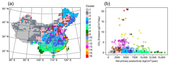
Figure 3.
K-means clustering results. (a) Distribution of clusters and (b) scatter plot of clusters.
2.2.4. Model Evaluation
We applied two metrics for model evaluation: the mean absolute error (MAE) and the determination coefficient (R2). The MAE was used to optimize the parameter in the GRNN during the training process. Both MAE and R2 were applied for model comparison during the testing process. These two measures are defined are follows:
where is the number of samples, is the observed value of the dependent variable, is the estimated value, and denotes the mean of the observed values.
3. Results
3.1. Characteristics of XCO2 Anomalies
First, we analyzed the characteristics of XCO2 anomalies derived from different methods for defining background XCO2 concentration. The CHN, LAT, and NE methods were applied to obtain the multi-year average XCO2 anomalies for China from 2015 to 2021. Figure 4 shows the spatial distributions of the XCO2 anomalies using these three approaches, along with the multi-year average CO2 emissions from the ODIAC dataset. Overall, the distributions of XCO2 anomalies derived from these three methods were found to be similar to those of the fossil fuel CO2 emissions, demonstrating the effectiveness of these methods in XCO2 enhancement. Specifically, high XCO2 anomaly values were found to be primarily distributed in the east and southeast regions of China, such as the Yangtze River Delta, the Pearl River Delta, and the North China Plain. In contrast, low XCO2 anomaly values were found in the west and northwest regions of China, such as the Tibetan Plateau and Inner Mongolia. Notably, the relatively high XCO2 anomaly values in southern Xinjiang Province were suggested to be related to the CO2 transport from the upper wind direction and retention effects within the Tarim Basin [42].
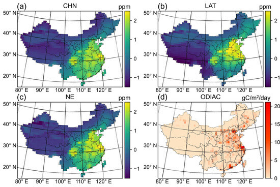
Figure 4.
Multi-year average XCO2 anomalies from three methods and CO2 emissions from 2015 to 2021. (a) CHN method, (b) LAT method, (c) NE method, and (d) CO2 emissions from ODIAC.
Several differences in XCO2 anomalies were observed when using the CHN, LAT, and NE methods. For instance, the positive XCO2 anomalies derived from the CHN method were lower than those from the LAT and NE methods. The LAT method emphasized higher XCO2 anomaly values in the North China Plain, while the NE method highlighted high XCO2 anomaly values in urban agglomerations, such as the Beijing–Tianjin–Hebei area, the Guangdong–Hong Kong–Macao Greater Bay area, the Sichuan-Chongqing area, and the lower reaches of the Yangtze River.
Next, we analyzed the correlation between the multi-year average XCO2 anomalies, derived from the CHN, LAT, and NE methods, and the ODIAC CO2 emissions. As shown in Figure 5, there was a positive correlation between XCO2 anomalies and CO2 emissions for each method, reaffirming the effectiveness of these methods in XCO2 enhancement. It was also observed that the relationships between XCO2 anomalies and CO2 emissions were nonlinear, primarily due to the influences of atmospheric transport and terrestrial ecosystems [6]. Atmospheric transport can cause CO2 from fossil fuel emissions to be carried to the surrounding areas, thereby enhancing the anthropogenic carbon emission signals in those regions. Simultaneously, plant photosynthesis can absorb part of the anthropogenic carbon emissions, thus weakening the signal [23].
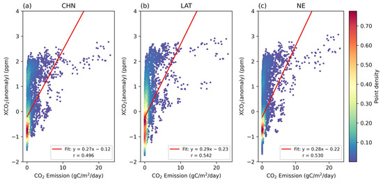
Figure 5.
Relationship between XCO2 anomalies from three methods and CO2 emissions. (a) CHN method, (b) LAT method, and (c) NE method. Color indicates point density.
In comparing the methods, the correlation coefficient between XCO2 anomalies and CO2 emissions derived from the CHN method was slightly lower than that from the LAT and NE methods. The CHN method, which utilized the same background XCO2 concentration across all grids, may not have fully captured the heterogeneous characteristics of background XCO2 concentration within China. In contrast, the LAT and NE methods accounted for these heterogeneous characteristics through latitudinal partition and information from the N-nearest non-emission grids, respectively. This suggests that XCO2 anomalies derived from the LAT and NE methods may facilitate the performance of the CO2 emission inversion model.
3.2. GRNN Performance in Modeling CO2 Emissions
As previously mentioned, anthropogenic CO2 emissions tend to exhibit heterogeneous and non-normal distribution. The main challenge in estimating these emissions from XCO2 enhancement lies in effectively modeling the underlying heterogeneity. We addressed this issue through four key aspects: (1) refining the XCO2 enhancement process; (2) incorporating population data; (3) implementing a partition modeling strategy; and (4) using the GRNN model. We divided the study area into several partitions using the K-means clustering method with ODIAC and NPP data and established a separate GRNN model for each partition. The inputs to the GRNN model included XCO2 anomalies, NPP, and population data, with XCO2 anomalies derived from the CHN, LAT, or NE methods. Since the number of partitions significantly influences model performance, we systematically tested the effectiveness of the three methods for background XCO2 concentration by varying the number of clusters () from 1 to 30. For each , the GRNN model was trained on data from 2015 to 2020 and tested on data in 2021.
Figure 6a,b illustrate the model’s performance (in terms of MAE and R2) with changes in the value of using the three XCO2 enhancement methods (CHN, LAT, and NE methods). The results show that, with a fixed XCO2 enhancement method, the R2 values initially increased sharply with an increase in k and then plateaued, while the MAE values decreased sharply before stabilizing. For instance, increasing the number of partitions from 1 to 30 using the NE method resulted in R2 values increasing from 0.932 to 0.985 and MAE values decreasing from 0.254 to 0.122 gC/m2/day. This indicates that the model’s performance improved with the partition modeling strategy, likely due to better accounting for the spatial heterogeneity in CO2 emissions. On the other hand, with a fixed , the CHN method generally performed the worst, consistent with the relationship shown in Figure 5. The LAT and NE methods yielded similar MAE values, but the NE method achieved higher R2 values.
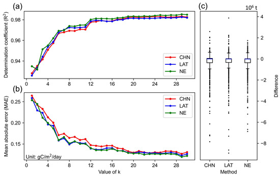
Figure 6.
Model performance with variations in . (a) R2, (b) MAE, and (c) difference between estimates and ODIAC data when = 30.
Figure 6c shows the differences between the CO2 emissions estimated by the GRNN model and the ODIAC data when the number of partitions was 30. For the CHN, LAT, and NE methods, the median differences were close to zero, and the interquartile range was from −5 × 10⁵ to 2 × 10⁴ t. Additionally, nearly 75 percent of differences were negative, indicating a tendency for the GRNN model to underestimate CO2 emissions. Among the three methods, the NE method showed a narrower range of difference, reflecting a more accurate estimation of CO2 emissions.
Furthermore, we investigated the influence of partition number on the error distribution. Figure S4 illustrates the differences between the GRNN-estimated CO2 emissions and the ODIAC data for varying values of (12, 16, 20, 24, and 30). For all three methods (CHN, LAT, and NE methods), the interquartile ranges of the differences remained largely negative across different values of , further indicating a consistent underestimation. However, as increased, the range of differences narrowed, suggesting improvements in model performance. Among the three methods, the NE method consistently showed the least degree of underestimation across different values of .
The spatial distributions of the estimated CO2 emissions and ODIAC data are shown in Figure 7a,b. The estimation was based on the NE method with 30 partitions; the results based on the CHN and LAT methods are presented in Figures S5 and S6. The estimation and the ODIAC data were found to exhibit similar spatial distribution, with high emission values distributed in the Yangtze River Delta, the Pearl River Delta, and the North China Plain. Figure 7c shows the differences between the CO2 emissions estimated by the GRNN model and those from the ODIAC data. Generally, the differences are less pronounced in western China compared to those in eastern China. The GRNN model tends to underestimate the CO2 emissions (indicated by red grids) in areas with high emissions, while overestimating them (indicated by blue grids) in areas with lower emissions, as evidenced in Figure 7c,d. This pattern, which might be introduced by atmospheric transport and/or the inherent characteristics of the GRNN, is consistent with findings from Yang et al. [21] and Zhang et al. [43]. We will discuss this further in Section 4.
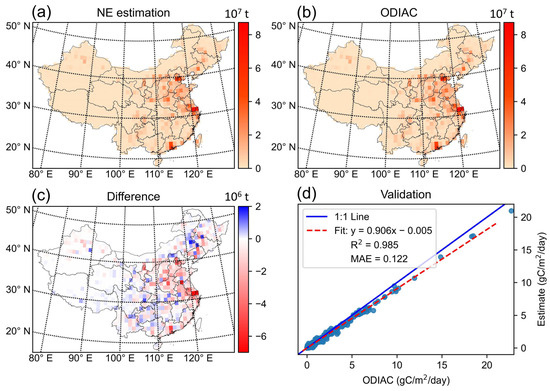
Figure 7.
The distribution of CO2 emissions and differences. (a) Estimated CO2 emissions from the GRNN model, (b) the ODIAC data, and (c) the difference between the estimates and ODIAC data. (d) Validation of the estimated CO2 emissions against ODIAC data for 2021. Note that the estimation is based on the NE method and = 30.
Compared to previous studies, our CO2 emission estimates have shown significant improvements. Yang et al. [21] estimated the CO2 emissions in China, with 71.0% of the discrepancies ranging from −1 × 10⁶ to 1 × 10⁶ t. Similarly, Mustafa et al. [22] estimated emissions over East Asia, reporting 84.0% of discrepancies within the same range. In contrast, our study found 86.5% of differences between −1 × 10⁶ and 1 × 10⁶ t. Figure 7d illustrates the relationship between the GRNN estimates and the ODIAC data, with a determination coefficient of 0.985, which is significantly higher than the values reported by Tan et al. [44] (R2 = 0.60), Yang et al. [21] (R2 = 0.65), and Zhang et al. [43] (R2 = 0.82).
4. Discussion
4.1. Influence of Different Variables on Model Performance
We investigated the influence of different variables on the performance of the GRNN model. We tested four groups of inputs: (1) XCO2 anomaly; (2) XCO2 anomaly and NPP; (3) XCO2 anomaly, NPP, and population; and (4) XCO2 anomaly, NPP, population, and nightlight data [45]. Figure 8 reveals the impact of incorporating these different variables on model performance, with the XCO2 anomaly derived from the NE method. Using only the XCO2 anomaly as input, the model performed the worst, with an R2 value of 0.497 and an MAE value of 0.664 gC/m2/day when the number of partitions was one (i.e., k = 1). As increased, model performance improved significantly, demonstrating the effectiveness of the partition modeling strategy again. The inclusion of the NPP dataset notably improved the model’s performance across all values, while the incorporation of population data further enhanced the effects. Between the two, population exhibited a relatively stronger impact on improving model accuracy. The incorporation of population data led to an increase in R2 values between 0.004 and 0.310 for different partitions and a decrease in MAE values between 0.036 and 0.269 gC/m2/day. The increase in R2 and decrease in MAE were particularly significant when population data were included, suggesting a strong link between CO2 emissions and human activities. The inclusion of the nightlight data did not lead to substantial performance gains, likely because nightlight and population data are closely correlated and may not need to be used simultaneously. Compared to previous studies [21,22], our GRNN model was significantly enhanced by incorporating population data and implementing a partition modeling strategy.
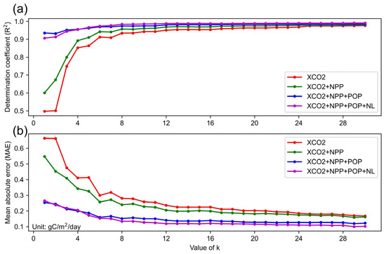
Figure 8.
The influence of different variables on model performance. (a) R2 and (b) MAE. The labels represent four groups of inputs: (1) XCO2 anomaly (red, XCO2 in short); (2) XCO2 anomaly and NPP (green, XCO2 + NPP in short); (3) XCO2 anomaly, NPP, and population (blue, XCO2 + NPP + POP in short); and (4) XCO2 anomaly, NPP, population, and nightlight data (purple, XCO2 + NPP + POP + NL in short).
4.2. Influence of Background XCO2 Concentration Definition on Model Performance
Anthropogenic CO2 emissions directly raise atmospheric CO2 concentrations, but atmospheric transport, diffusion, and absorption by natural sinks complicate the relationship, making it challenging to trace the exact source and magnitude of emissions based solely on CO2 concentration observations [6,20,22]. As a result, several previous studies have emphasized that an appropriate definition of background XCO2 concentration is crucial to the extraction of anthropogenic CO2 emission signals as well as to the estimation of CO2 emissions [19,20,23].
In this study, we employed three different methods to derive background XCO2 concentration: the CHN, LAT, and NE methods. From the perspectives of XCO2 anomaly distribution and CO2 emission estimation, the NE method either outperformed or was at least comparable to the LAT method, while the CHN method performed the worst. The CHN and LAT methods define background regions based on the entire area of China and 10-degree latitudinal bands, respectively. However, these regions may include or be influenced by areas with significant CO2 emissions, leading to potential contamination of the background signal. The NE method, which originates from the regional comparison methods, appears to be most effective in extracting the anthropogenic carbon emission signals from the XCO2 observations in this study. It outperformed the CHN and LAT methods, as evidenced by a narrower range of differences and a lower degree of underestimation (Figure 6 and Figure S4). By selecting the N-nearest non-emission grids as the background region, the NE method effectively minimized the interference of anthropogenic CO2 emissions and revealed the real/intrinsic distribution of the background XCO2 concentration. These findings underscore the importance of defining background regions with minimal anthropogenic impact in order to accurately extract anthropogenic CO2 emission signals.
While our current work focuses on evaluating different definitions of background XCO2 concentration, variations in background values within a given method may also have a significant impact on model outputs. Conducting a sensitivity analysis could provide valuable insights into the influence of this variable, and we consider this a promising direction for future research.
4.3. Distribution of Differences
The GRNN model exhibited a tendency to underestimate CO2 emissions in areas with high emissions while overestimating them in areas with lower emissions. To better understand this pattern, we further explored the underlying reasons. Figure 9 illustrates the relationship between the differences in emission estimates and the ODIAC data. Generally, underestimation was more prevalent than overestimation. Specifically, areas with high CO2 emissions were more likely to produce underestimated results, whereas grids with low emissions tended to yield overestimated results. This pattern might be attributed to atmospheric transport and/or the inherent characteristics of the GRNN model.
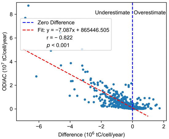
Figure 9.
Relationship between estimation differences and ODIAC data.
First, due to atmospheric transport, carbon dioxide diffuses from high-emission areas to surrounding low-emission areas, leading to an underestimation of CO2 emissions in the former and an overestimation in the latter. Zhang et al. [43], using a similar neural network model, observed an underestimation of CO2 emissions in megacities, such as Beijing, Shanghai, and Guangzhou. Similarly, Yang et al. [21] reported an overestimation in low-emission areas, attributing it to the elevated CO2 concentrations caused by nearby large emitting sources, which spread through atmospheric transport to adjacent regions with lower emissions. Second, the underestimation of CO2 emissions may be related to the inherent characteristics of the GRNN model. The GRNN model essentially performs probability density estimation for new inputs based on existing data, meaning that the estimation is constrained by the observed minimum and maximum values [40]. When the GRNN model was applied for predictions, samples from high-emission areas were fewer in number and more sparsely distributed in the Euclidean space than those from low-emission areas. As a result, the GRNN model was more likely to learn the parameter from the previous years’ data within the same region. Considering the tendency for annual CO2 emissions to show an increasing trend across China in recent years, the characteristics of the GRNN model led to this underestimation in high-emission areas.
In addition, since the model was calibrated using data from 2015 to 2020 and validated against 2021 data, it is important to discuss whether the COVID-19 pandemic affected the model’s performance. Global CO2 emissions declined by 8.8% in the first half of 2020 due to the pandemic-related restrictions [46]. In China, emissions dropped significantly between January and April 2020 but quickly rebounded to pre-pandemic levels [47], resulting in a slight overall increase in emissions for 2020 and a substantial rise in 2021. Although the GRNN model did not include a variable to account for the COVID-19 pandemic, the XCO2 observations used in the model might have implicitly captured its impact. Consequently, the model maintained reasonable performance despite these fluctuations. Nonetheless, a more detailed investigation is needed to fully understand and quantify the effects of COVID-19 pandemic on model accuracy.
4.4. Future Directions for Research
In this study, we applied three approaches to derive the XCO2 anomaly and the GRNN model to estimate CO2 emissions, with promising results. However, there are several limitations in this study which can be addressed for further improvements. First, although we compared the differences in XCO2 anomalies and model performance between the three approaches (CHN, LAT, and NE methods) for defining the background XCO2 concentration, none of these methods considered the influences from atmospheric transport and topographical factors. For instance, atmospheric transport can cause CO2 to diffuse from high-emission areas to surrounding low-emission areas, while basin topography can lead to the retention of CO2 [17]. These factors should be fully accounted for to improve the model further. Second, the availability of full-coverage, precise satellite XCO2 observations would significantly improve the estimation of CO2 emissions based on remote sensing. In this study, we utilized the OCO-2 GEOS Level 3 data to estimate CO2 emissions in China. However, due to the limitations in precision and spatiotemporal coverage of the OCO-2 satellite, we were unable to estimate CO2 emissions with finer spatiotemporal resolution at the city scale [48]. Upcoming carbon satellite missions with wider swaths, such as the European Sentinel satellites with a minimum of 250 km swath, hold the potential to provide full-coverage XCO2 observations with high precision [25]. This advancement will enable more accurate monitoring and estimation of CO2 emissions at regional, megacity, and point-source geographical scales.
5. Conclusions
In this study, we applied the GRNN model and a partition modeling strategy to estimate anthropogenic CO2 emissions in China using remote sensing data. We evaluated three approaches to extract the anthropogenic CO2 emission signals from XCO2 observations. To address the high heterogeneity and non-normal distribution features of CO2 emissions, we applied the K-means clustering algorithm to divide the study area into several partitions and then established a separate GRNN model for each partition. The GRNN model used the XCO2 anomalies, NPP, and population data as inputs, with ODIAC data as output. The results demonstrate that the NE method either outperformed or was at least comparable to the LAT method, while the CHN method performed the worst. Implementing the partition modeling strategy and incorporating population data significantly improved the GRNN model’s performance. Specifically, increasing the number of partitions from 1 to 30 using the NE method resulted in R2 values increasing from 0.932 to 0.985, while MAE values decreased from 0.254 to 0.122 gC/m2/day. The inclusion of population data led to an increase in R2 values between 0.004 and 0.310 for different partitions under the NE method and a reduction in MAE values between 0.036 and 0.269 gC/m2/day. The GRNN model tended to underestimate CO2 emissions in areas with high emissions while overestimating them in areas with lower emissions, a pattern likely influenced by atmospheric CO2 transport and/or the inherent characteristics of the GRNN. The methods and findings of this study will contribute to a better understanding of XCO2 enhancement and provide effective methodologies for improving the estimation of anthropogenic CO2 emissions based on remote sensing. Moreover, this study is particularly useful for estimating carbon emissions at national or regional scales, which is crucial for the government in setting targets and formulating policies.
Supplementary Materials
The following supporting information can be downloaded at https://www.mdpi.com/article/10.3390/atmos16060631/s1: Figure S1: Box plots showing the distributions of XCO2 concentrations and ODIAC fossil fuel CO2 emissions in China from 2015 to 2021; Figure S2: Relationship between CO2 emissions and population in China; Figure S3: Model performance with 5, 10, and 15-nearest non-emission grids for the NE method. (a) R2 and (b) MAE; Figure S4: Difference between estimates and ODIAC data when = 12, 16, 20, 24, and 30; Figure S5: The distribution of CO2 emissions and difference. (a) Estimated CO2 emissions from the GRNN model, (b) the ODIAC data, and (c) the difference between the estimates and ODIAC data. (d) Validation of the estimated CO2 emissions against ODIAC data for 2021. Note that the estimation is based on the CHN method and = 30; Figure S6: The distribution of CO2 emissions and difference. (a) Estimated CO2 emissions from the GRNN model, (b) the ODIAC data, and (c) the difference between the estimates and ODIAC data. (d) Validation of the estimated CO2 emissions against ODIAC data for 2021. Note that the estimation is based on the LAT method and = 30.
Author Contributions
Conceptualization, C.C. and B.S.; formal analysis, C.C., K.Q., and S.W.; funding acquisition, C.C.; investigation, K.Q., S.W., C.Z., and J.L.; methodology, C.C.; software, K.Q. and S.W.; supervision, C.C.; validation, C.C., K.Q., S.W., and C.Z.; visualization, K.Q., S.W., and C.Z.; writing—original draft, C.C., K.Q., and S.W.; writing—review and editing, C.C., B.S., and J.L. All authors have read and agreed to the published version of the manuscript.
Funding
This work was funded by the Open Research Fund Program of State Key Laboratory of Hydroscience and Engineering (sklhse-2023-A-07), the Open Research Fund Program of Key Laboratory of the Hydrosphere of the Ministry of Water Resources (mklhs-2023-02), the Basic and Applied Basic Research Foundation of Guangdong Province (2021A1515110768), the National Key Research and Development Program of China (2023YFC3206700), and the Guangdong Provincial Key Laboratory of Intelligent Disaster Prevention and Emergency Technologies for Urban Lifeline Engineering (2022B1212010016).
Institutional Review Board Statement
Not applicable.
Informed Consent Statement
Not applicable.
Data Availability Statement
The original contributions presented in this study are included in the article/Supplementary Materials. Further inquiries can be directed to the corresponding author(s).
Acknowledgments
We acknowledge Tiejian Li of Tsinghua University and Songdong Shao of Dongguan University of Technology for their valuable and constructive suggestions in improving the paper.
Conflicts of Interest
The authors declare no conflicts of interest.
References
- Milly, P.C.; Betancourt, J.; Falkenmark, M.; Hirsch, R.M.; Kundzewicz, Z.W.; Lettenmaier, D.P.; Stouffer, R.J. Stationarity is dead: Whither water management? Science 2008, 319, 573–574. [Google Scholar] [CrossRef] [PubMed]
- Zemp, M.; Huss, M.; Thibert, E.; Eckert, N.; McNabb, R.; Huber, J.; Barandun, M.; Machguth, H.; Nussbaumer, S.U.; Gärtner-Roer, I. Global glacier mass changes and their contributions to sea-level rise from 1961 to 2016. Nature 2019, 568, 382–386. [Google Scholar] [CrossRef] [PubMed]
- Zhang, W.; Zhou, T.; Wu, P. Anthropogenic amplification of precipitation variability over the past century. Science 2024, 385, 427–432. [Google Scholar] [CrossRef]
- Huang, Y.; Wang, Y.; Peng, J.; Li, F.; Zhu, L.; Zhao, H.; Shi, R. Can China achieve its 2030 and 2060 CO2 commitments? Scenario analysis based on the integration of LEAP model with LMDI decomposition. Sci. Total Environ. 2023, 888, 164151. [Google Scholar] [CrossRef]
- Solomon, S.; Plattner, G.-K.; Knutti, R.; Friedlingstein, P. Irreversible climate change due to carbon dioxide emissions. Proc. Natl. Acad. Sci. USA 2009, 106, 1704–1709. [Google Scholar] [CrossRef]
- Labzovskii, L.D.; Jeong, S.-J.; Parazoo, N.C. Working towards confident spaceborne monitoring of carbon emissions from cities using Orbiting Carbon Observatory-2. Remote Sens. Environ. 2019, 233, 111359. [Google Scholar] [CrossRef]
- Zheng, B.; Cheng, J.; Geng, G.; Wang, X.; Li, M.; Shi, Q.; Qi, J.; Lei, Y.; Zhang, Q.; He, K. Mapping anthropogenic emissions in China at 1 km spatial resolution and its application in air quality modeling. Sci. Bull. 2021, 66, 612–620. [Google Scholar] [CrossRef]
- Ballantyne, A.P.; Alden, C.B.; Miller, J.B.; Tans, P.P.; White, J.W.C. Increase in observed net carbon dioxide uptake by land and oceans during the past 50 years. Nature 2012, 488, 70–72. [Google Scholar] [CrossRef]
- Liu, Z.; Deng, Z.; Huang, X. A carbon-monitoring strategy through near-real-time data and space technology. Innovation 2023, 4, 100346. [Google Scholar] [CrossRef]
- Guan, D.; Liu, Z.; Geng, Y.; Lindner, S.; Hubacek, K. The gigatonne gap in China’s carbon dioxide inventories. Nat. Clim. Change 2012, 2, 672–675. [Google Scholar] [CrossRef]
- Cogan, A.J.; Boesch, H.; Parker, R.J.; Feng, L.; Palmer, P.I.; Blavier, J.F.L.; Deutscher, N.M.; Macatangay, R.; Notholt, J.; Roehl, C.; et al. Atmospheric carbon dioxide retrieved from the Greenhouse gases Observing SATellite (GOSAT): Comparison with ground-based TCCON observations and GEOS-Chem model calculations. J. Geophys. Res. Atmos. 2012, 117, D21301. [Google Scholar] [CrossRef]
- Hammerling, D.M.; Michalak, A.M.; Kawa, S.R. Mapping of CO2 at high spatiotemporal resolution using satellite observations: Global distributions from OCO-2. J. Geophys. Res. Atmos. 2012, 117, D6. [Google Scholar] [CrossRef]
- Peiro, H.; Crowell, S.; Schuh, A.; Baker, D.F.; O’Dell, C.; Jacobson, A.R.; Chevallier, F.; Liu, J.; Eldering, A.; Crisp, D.; et al. Four years of global carbon cycle observed from the Orbiting Carbon Observatory 2 (OCO-2) version 9 and in situ data and comparison to OCO-2 version 7. Atmos. Chem. Phys. 2022, 22, 1097–1130. [Google Scholar] [CrossRef]
- Yang, D.X.; Liu, Y.; Cai, Z.N.; Chen, X.; Yao, L.; Lu, D.R. First global carbon dioxide maps produced from TanSat measurements. Adv. Atmos. Sci. 2018, 35, 621–623. [Google Scholar] [CrossRef]
- Kort, E.A.; Frankenberg, C.; Miller, C.E.; Oda, T. Space-based observations of megacity carbon dioxide. Geophys. Res. Lett. 2012, 39, L17806. [Google Scholar] [CrossRef]
- Schwandner, F.M.; Gunson, M.R.; Miller, C.E.; Carn, S.A.; Eldering, A.; Krings, T.; Verhulst, K.R.; Schimel, D.S.; Nguyen, H.M.; Crisp, D. Spaceborne detection of localized carbon dioxide sources. Science 2017, 358, eaam5782. [Google Scholar] [CrossRef]
- Hakkarainen, J.; Ialongo, I.; Tamminen, J. Direct space-based observations of anthropogenic CO2 emission areas from OCO-2. Geophys. Res. Lett. 2016, 43, 400–411, 406. [Google Scholar] [CrossRef]
- Reuter, M.; Buchwitz, M.; Schneising, O.; Krautwurst, S.; O’Dell, C.W.; Richter, A.; Bovensmann, H.; Burrows, J.P. Towards monitoring localized CO2 emissions from space: Co-located regional CO2 and NO2 enhancements observed by the OCO-2 and S5P satellites. Atmos. Chem. Phys. 2019, 19, 9371–9383. [Google Scholar] [CrossRef]
- Wu, D.; Lin, J.C.; Fasoli, B.; Oda, T.; Ye, X.; Lauvaux, T.; Yang, E.G.; Kort, E.A. A Lagrangian approach towards extracting signals of urban CO2 emissions from satellite observations of atmospheric column CO2 (XCO2): X-Stochastic Time-Inverted Lagrangian Transport model (“X-STILT v1”). Geosci. Model Dev. 2018, 11, 4843–4871. [Google Scholar] [CrossRef]
- Pei, Z.; Han, G.; Ma, X.; Shi, T.; Gong, W. A method for estimating the background column concentration of CO2 using the lagrangian approach. IEEE Trans. Geosci. Remote Sens. 2022, 60, 1–12. [Google Scholar] [CrossRef]
- Yang, S.; Lei, L.; Zeng, Z.; He, Z.; Zhong, H. An assessment of anthropogenic CO2 emissions by satellite-based observations in China. Sensors 2019, 19, 1118. [Google Scholar] [CrossRef]
- Mustafa, F.; Bu, L.; Wang, Q.; Yao, N.; Shahzaman, M.; Bilal, M.; Aslam, R.W.; Iqbal, R. Neural-network-based estimation of regional-scale anthropogenic CO2 emissions using an Orbiting Carbon Observatory-2 (OCO-2) dataset over East and West Asia. Atmos. Meas. Tech. 2021, 14, 7277–7290. [Google Scholar] [CrossRef]
- Wang, Y.; Wang, M.; Teng, F.; Ji, Y. Remote sensing monitoring and analysis of spatiotemporal changes in China’s anthropogenic carbon emissions based on XCO2 data. Remote Sens. 2023, 15, 3207. [Google Scholar] [CrossRef]
- Wilmot, T.Y.; Lin, J.C.; Wu, D.; Oda, T.; Kort, E.A. Toward a satellite-based monitoring system for urban CO2 emissions in support of global collective climate mitigation actions. Environ. Res. Lett. 2024, 19, 084029. [Google Scholar] [CrossRef]
- Pan, G.; Xu, Y.; Ma, J. The potential of CO2 satellite monitoring for climate governance: A review. J. Environ. Manag. 2021, 277, 111423. [Google Scholar] [CrossRef]
- Zhang, Y.; Liu, X.; Lei, L.; Liu, L. Estimating global anthropogenic CO2 gridded emissions using a data-driven stacked random forest regression model. Remote Sens. 2022, 14, 3899. [Google Scholar] [CrossRef]
- Ji, Z.; Song, H.; Lei, L.; Sheng, M.; Guo, K.; Zhang, S. A novel approach for predicting anthropogenic CO2 emissions using machine learning based on clustering of the CO2 concentration. Atmosphere 2024, 15, 323. [Google Scholar] [CrossRef]
- Zhang, J.X.; Zhang, H.; Wang, R.; Zhang, M.X.; Huang, Y.Z.; Hu, J.H.; Peng, J.Y. Measuring the critical influence factors for predicting carbon dioxide emissions of expanding megacities by XGBoost. Atmosphere 2022, 13, 599. [Google Scholar] [CrossRef]
- Uyar, N.; Uyar, A. Assessing climate change impacts on cropland and greenhouse gas emissions using remote sensing and machine learning. Atmosphere 2025, 16, 418. [Google Scholar] [CrossRef]
- Li, X.; Zhang, X. A comparative study of statistical and machine learning models on carbon dioxide emissions prediction of China. Environ. Sci. Pollut. Res. 2023, 30, 117485–117502. [Google Scholar] [CrossRef]
- Rosenzweig, C.; Solecki, W.; Hammer, S.A.; Mehrotra, S. Cities lead the way in climate–change action. Nature 2010, 467, 909–911. [Google Scholar] [CrossRef]
- Weir, B.; Ott, L.; Team, O.-S. OCO-2 GEOS Level 3 Daily, 0.5 x 0.625 Assimilated CO2 V10r; Goddard Earth Sciences Data and Information Services Center: Greenbelt, MD, USA, 2022. [Google Scholar] [CrossRef]
- Running, S.; Zhao, M. MODIS/Terra Net Primary Production Gap-Filled Yearly L4 Global 500 m SIN Grid V061; NASA EOSDIS Land Processes Distributed Active Archive Center: Sioux Falls, SD, USA, 2021. [Google Scholar] [CrossRef]
- Sims, K.; Reith, A.; Bright, E.; Kaufman, J.; Pyle, J.; Epting, J.; Gonzales, J.; Adams, D.; Powell, E.; Urban, M.; et al. LandScan Global 2022; Oak Ridge National Laboratory: Oak Ridge, TN, USA, 2023. [Google Scholar] [CrossRef]
- Oda, T.; Maksyutov, S.; Andres, R.J. The Open-source Data Inventory for Anthropogenic CO2, version 2016 (ODIAC2016): A global monthly fossil fuel CO2 gridded emissions data product for tracer transport simulations and surface flux inversions. Earth Syst. Sci. Data 2018, 10, 87–107. [Google Scholar] [CrossRef]
- Sheng, M.; Lei, L.; Zeng, Z.-C.; Rao, W.; Zhang, S. Detecting the responses of CO2 column abundances to anthropogenic emissions from satellite observations of GOSAT and OCO-2. Remote Sens. 2021, 13, 3524. [Google Scholar] [CrossRef]
- Wang, H.; Gong, F.-Y.; Newman, S.; Zeng, Z.-C. Consistent weekly cycles of atmospheric NO2, CO, and CO2 in a North American megacity from ground-based, mountaintop, and satellite measurements. Atmos. Environ. 2022, 268, 118809. [Google Scholar] [CrossRef]
- Golkar, F.; Mousavi, S.M. Variation of XCO2 anomaly patterns in the Middle East from OCO-2 satellite data. Int. J. Digital Earth 2022, 15, 1219–1235. [Google Scholar] [CrossRef]
- Hakkarainen, J.; Ialongo, I.; Maksyutov, S.; Crisp, D. Analysis of four years of global XCO2 anomalies as seen by Orbiting Carbon Observatory-2. Remote Sens. 2019, 11, 850. [Google Scholar] [CrossRef]
- Specht, D.F. A general regression neural network. IEEE Trans. Neural Networks 1991, 2, 568–576. [Google Scholar] [CrossRef]
- Ikotun, A.M.; Ezugwu, A.E.; Abualigah, L.; Abuhaija, B.; Heming, J. K-means clustering algorithms: A comprehensive review, variants analysis, and advances in the era of big data. Inf. Sci. 2023, 622, 178–210. [Google Scholar] [CrossRef]
- Aminu, M.D.; Nabavi, S.A.; Rochelle, C.A.; Manovic, V. A review of developments in carbon dioxide storage. Appl. Energy 2017, 208, 1389–1419. [Google Scholar] [CrossRef]
- Zhang, S.Q.; Lei, L.P.; Song, H.; Guo, K.Y.; Ji, Z.H.; Sheng, M.Y. A neural network partitioning method for carbon emission estimation based on spatial-temporal clustering of atmospheric CO2 concentration. China Environ. Sci. 2023, 43, 5604–5613. [Google Scholar] [CrossRef]
- Tan, Y.B.; Wang, S.S.; Xue, R.B.; Zhang, S.B.; Wang, T.Y.; Liu, J.Q.; Zhou, B. Estimation of carbon emissions in various clustered regions of China based on OCO-2 satellite XCO2 data and random forest modelling. Atmos. Environ. 2024, 338, 120860. [Google Scholar] [CrossRef]
- Elvidge, C.D.; Zhizhin, M.; Ghosh, T.; Hsu, F.C.; Taneja, J. Annual time series of global VIIRS nighttime lights derived from monthly averages: 2012 to 2019. Remote Sens. 2021, 13, 922. [Google Scholar] [CrossRef]
- Liu, Z.; Ciais, P.; Deng, Z.; Lei, R.X.; Davis, S.J.; Feng, S.; Zheng, B.; Cui, D.; Dou, X.Y.; Zhu, B.Q.; et al. Near-real-time monitoring of global CO2 emissions reveals the effects of the COVID-19 pandemic. Nat. Commun. 2020, 11, 5172. [Google Scholar] [CrossRef]
- Zheng, B.; Geng, G.N.; Ciais, P.; Davis, S.J.; Martin, R.V.; Meng, J.; Wu, N.N.; Chevallier, F.; Broquet, G.; Boersma, F.; et al. Satellite-based estimates of decline and rebound in China’s CO2 emissions during COVID-19 pandemic. Sci. Adv. 2020, 6, eabd4998. [Google Scholar] [CrossRef]
- Zhang, M.; Liu, G. Mapping contiguous XCO2 by machine learning and analyzing the spatio-temporal variation in China from 2003 to 2019. Sci. Total Environ. 2023, 858, 159588. [Google Scholar] [CrossRef]
Disclaimer/Publisher’s Note: The statements, opinions and data contained in all publications are solely those of the individual author(s) and contributor(s) and not of MDPI and/or the editor(s). MDPI and/or the editor(s) disclaim responsibility for any injury to people or property resulting from any ideas, methods, instructions or products referred to in the content. |
© 2025 by the authors. Licensee MDPI, Basel, Switzerland. This article is an open access article distributed under the terms and conditions of the Creative Commons Attribution (CC BY) license (https://creativecommons.org/licenses/by/4.0/).