Influence of Satellite and Presatellite Periods on the Validation of Major Sudden Stratospheric Warmings in Historical CMIP5 Simulations

Abstract

This study assesses the ability of fourteen CMIP5 climate models to reproduce the main characteristics of major stratospheric sudden warmings (SSWp) in historical simulations. Model performance is evaluated through comparisons with three reanalysis datasets, considering two periods: the satellite era (1979–2005) and an extended period including pre-satellite years (1958–2005). Results show that model consistency with reanalyses is significantly higher during the satellite period, with up to seven models showing no statistically significant differences (p > 0.05) in at least eight out of ten key diagnostics. In contrast, performance decreases in the extended period, likely due to greater observational uncertainty. A systematic overrepresentation of displacement-type events (SSW_D) was found in most models, compared to the split-type dominance in reanalysis data. These findings highlight the importance of the validation period and event classification in model evaluation and establish a robust framework for future comparisons using CMIP6 models and newer reanalysis products.

1. Introduction

The stratospheric polar vortex is a system of westerly zonal winds that dominates the circulation at high latitudes during the Boreal winter [1,2,3,4,5]. Related to it, stratospheric sudden warmings (SSWs) are defined as events characterized by a rapid reversal of the zonal wind direction in the polar stratosphere, typically accompanied by an abrupt temperature increase in that region. According to the standard classification [6], SSWs can be categorized as either minor or major. Minor events are associated with a substantial warming in the polar stratosphere but without a reversal of the zonal-mean zonal wind at 60° N and 10 hPa. In contrast, major SSWs (SSWm) are defined by a complete wind reversal from westerly to easterly at those latitudes and pressure levels. A detailed understanding of the dynamical mechanisms driving SSWs remains one of the primary scientific challenges in contemporary atmospheric research [7,8,9,10,11].

Given their relevance for the weather and the need to have a good representation of them in global climate models, SSWs have been analyzed in the past from reanalyses and models, both through simulations using individual climate models and within the framework of multimodel intercomparison projects. Notable among these are the Coupled Model Intercomparison Project (CMIP) [12,13,14,15,16,17] and the Chemistry–Climate Model Initiative (CCMI) [6,18]. 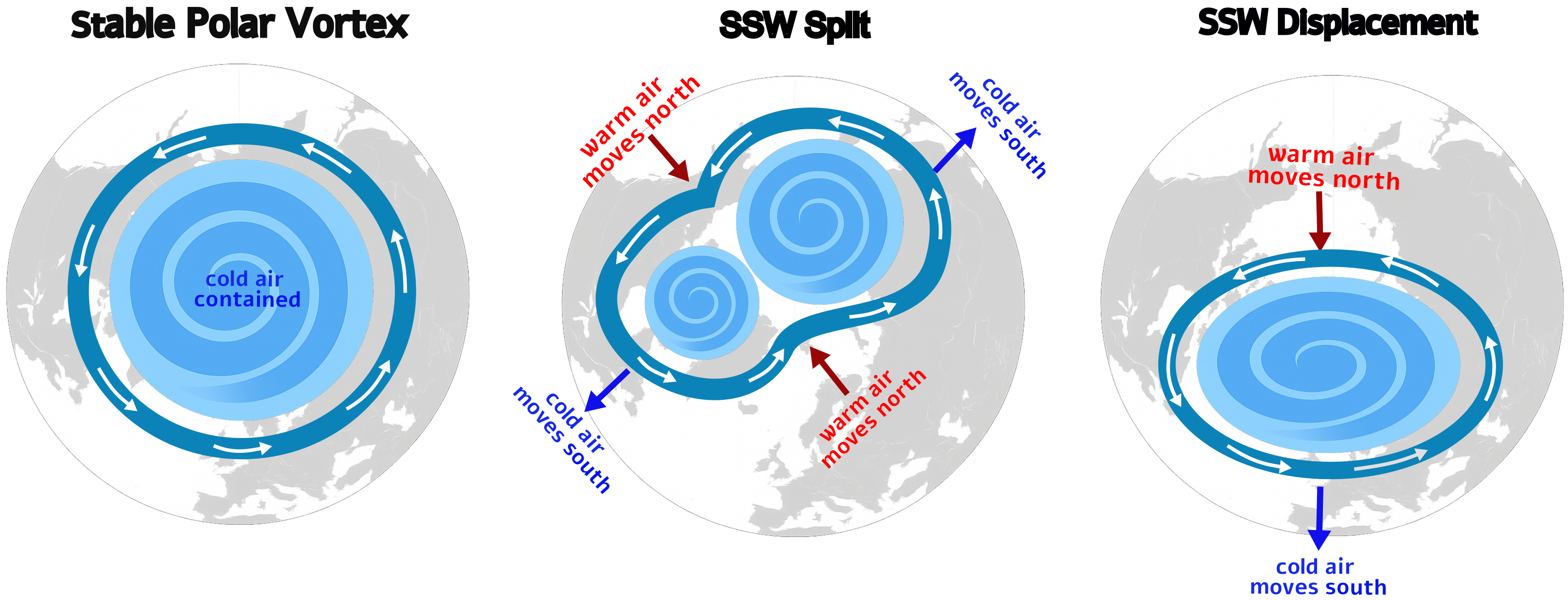Several studies have shown that discrepancies between models and reanalysis data in the frequency of SSWm occurrence are closely linked to key dynamical factors, particularly the climatological mean and variability of the polar stratospheric zonal wind [17,19]. During SSWs, the zonal winds in the polar stratosphere reverse direction, which can lead to either displacements ($SS{W}_D$) or splits ($SS{W}_S$) of the polar vortex. These two categories are predominantly associated with the vertical propagation of planetary Rossby waves: $SS{W}_D$ are generally dominated by wave number 1, while $SS{W}_S$ are associated with wave number 2 [8,20,21,22,23,24,25]. A schematic representation of these configurations is shown in Figure 1.

Few multimodel studies have explicitly addressed SSWm classification into $SS{W}_D$ and $SS{W}_S$ events. However, existing investigations report significant differences in the internal dynamics associated with each type. In particular, the tropospheric response following $SS{W}_S$ events is generally more intense than that observed after $SS{W}_D$ events [15]. Additionally, $SS{W}_S$ events have consistently been shown to exhibit a predominantly barotropic structure throughout the stratosphere, whereas $SS{W}_D$ events tend to display a more baroclinic structure [14,26,27].

The results of any evaluation of SSWm representation in climate models are highly sensitive to the reference datasets and period of study used. Specifically, the temporal length of the time series and the vertical configuration of the model—such as its top level and vertical resolution—have a critical impact on the resulting statistics [12,27,28]. This aspect, which has received limited attention in recent assessments, is addressed in detail in the present study, using various CMIP5 models and multiple reanalyses.

The validation of climate models against reanalysis datasets must consider the differences in data quality between the satellite and pre-satellite eras. Before 1979, reanalyses relied exclusively on in situ observations, which were sparse and unevenly distributed, especially in the Southern Hemisphere, leading to greater uncertainties in the representation of atmospheric dynamics [29,30,31]. Several studies have shown that discrepancies between reanalysis products are notably larger during the pre-satellite period, particularly in the depiction of stratospheric variability and mid-latitude atmospheric waves [32,33,34]. These limitations must be taken into account when interpreting model performance across different periods, highlighting the importance of validating models not only during the well-observed satellite era but also under the more uncertain conditions of the pre-satellite period.

The main objective of this study is to assess how the selection of the validation period (satellite vs. pre-satellite) affects the ability of climate models to accurately reproduce SSWm. This study proposes that the evaluation of climate models’ ability to reproduce the dynamics of SSWm, based on comparisons with historical reanalysis data, is strongly conditioned by the chosen time period. While the choice of reanalysis product can also affect the results, it is expected that the selected historical period—whether pre-satellite or satellite—exerts an even greater influence due to substantial differences in data quality and observational coverage between the two periods. Therefore, a comparative analysis of climate models must explicitly consider two key factors: the selected historical period (pre-satellite vs. satellite) and the reanalysis dataset used to evaluate the results from the models, in order to produce more robust and representative results. To this end, we conduct a detailed evaluation of the ability of high-top CMIP5 models to reproduce fundamental features of SSWm. This assessment employs three distinct reanalyses, only one of which spans the full pre-satellite period (1958–2005).

Furthermore, the results presented here may serve as a baseline for future studies aimed at evaluating improvements achieved by the new generation of climate models participating in present and future phases of the CMIP, particularly with regard to the detailed representation of stratospheric dynamics associated with SSWm [19,26,35].

Despite previous efforts to evaluate the representation of stratospheric sudden warmings (SSW) in climate models, few studies have systematically assessed the influence of the validation period on model performance, particularly considering differences in observational coverage between the satellite and pre-satellite eras. Addressing this gap is crucial for improving the robustness of model evaluations and for understanding potential biases in historical climate simulations. The goal of this study is to quantify how the selected validation period affects the ability of CMIP5 models to reproduce SSWm using multiple reanalysis datasets. By providing a detailed assessment across different periods and reanalyses, this work contributes to a more rigorous understanding of model performance, supporting future improvements in the simulation of stratospheric dynamics and their coupling with tropospheric processes.

2. Data and Methods

This study uses daily data of air temperature, geopotential height, and zonal wind from fourteen climate models participating in the CMIP5 (see

Table 1. CMIP5 models used in this study.

	Model	Center	Horizontal Resolution (lat × lon)	Vertical Levels	Model Top (km)
1	CanESM2	CCCma	1.88 × 0.94	35	48.1
2	CMCC-CESM	CMCC	3.44 × 3.75	39	80.6
3	CMCC-CMS	CMCC	3.71 × 3.75	95	80.6
4	GFDL-CM3	GFDL	1.25 × 2.50	39	76.3
5	HadGEM2-CC	Met Office	1.25 × 1.87	96	84.1
6	IPSL-CM5A-LR	IPSL	1.89 × 3.79	39	70.4
7	IPSL-CM5A-MR	IPSL	1.25 × 2.52	39	70.4
8	IPSL-CM5B-LR	IPSL	1.89 × 3.79	39	70.4
9	MIROC-ESM-CHEM	AORI/NIES/JAMSTEC	2.81 × 1.41	80	87.8
10	MPI-ESM-LR	MPI-M	1.88 × 0.94	47	80.6
11	MPI-ESM-MR	MPI-M	1.88 × 0.94	47	80.6
12	MPI-ESM-P	MPI-M	1.88 × 0.94	47	80.6
13	MRI-CGCM3	MRI	0.75 × 0.38	48	80.6
14	MRI-ESM1	MRI	0.75 × 0.38	48	80.6

Note: Full names of modeling centers are provided in the Abbreviations section.

). These models are considered high-top models, with the exception of CanESM2, which is considered a mid-top model [12,13,14,16,36,37]. Low-top models are not included here since previous studies have shown that they poorly represent key stratospheric processes, such as SSWm [12,13].

For model validation, potential discrepancies associated with the choice of reanalysis are taken into account. Three reanalyses commonly used in stratospheric studies, due to their reliability in this region, are selected: ERA-Interim [38], MERRA [39], and JRA-55 [40,41]. These reanalyses are selected because they were the standard products used in the stratospheric research community at the time when CMIP5 simulations were widely analyzed. Their temporal overlap with the historical simulations of CMIP5 (ending in 2005) and their frequent use in benchmark SSWm studies [14,42] make them the most appropriate datasets for this comparative evaluation.

To ensure robustness in the analysis, particular attention is given to the influence of the selected historical period on model evaluation. Two distinct periods are defined: the first covers only the satellite era (1979–2005), during which all three reanalyses (ERA-Interim, MERRA, and JRA-55) are used simultaneously; the second spans a longer interval (1958–2005), for which only JRA-55 is available, due to its extended historical coverage [40,41]. This methodology allows for the identification of climate models whose representation of SSWm is consistent regardless of the time period considered.

The detection of SSWm events is typically based on two widely accepted methods: the definition proposed by the World Meteorological Organization (WMO) and the criterion introduced by Charlton and Polvani (hereafter CP07) [42,43]. According to the WMO, a SSWm occurs when the zonal-mean zonal wind at 60° N and 10 hPa reverses from westerly to easterly, accompanied by a rapid and significant increase in polar stratospheric temperature. Charlton and Polvani [42] proposed a simplified detection method that relies solely on the zonal wind reversal, arguing that the warming is implicitly captured by the wind dynamics. Previous studies have shown that both criteria yield very similar results, with no significant differences in the frequency of identified events [18,42]. In this work, we specifically apply the CP07 criterion, which defines an SSWm event in the Northern Hemisphere (NH) as occurring when the zonal-mean zonal wind at 60° N and 10 hPa reverses from westerly to easterly during the November–March period. The day of reversal is considered the central date of the event, which ends when the zonal wind returns to its original (westerly) direction.

To assess whether the annual frequencies of SSWm simulated by each climate model are statistically consistent with those observed in the reanalysis datasets, the Student’s t-test is applied, using significance levels of 0.05 and 0.10, following the methodology described by Charlton et al. [6].

The analysis focuses on five key characteristics of SSWm: (1) the annual frequency of occurrence, computed as the number of events per winter; (2) the morphological classification into $SS{W}_D$ and $SS{W}_S$ events, based on the polar vortex configuration at 10 hPa; (3) the event duration, defined from the reversal of the zonal wind at 60° N and 10 hPa until its return to westerly values; (4) the deceleration of the polar jet, quantified as the change in the zonal-mean wind speed ($\Delta U_{10}$) around the event onset; and (5) the temperature anomalies over the polar cap at 10 hPa and 100 hPa. These metrics are computed using both reanalysis datasets and CMIP5 model outputs to allow a comprehensive comparison across different time periods.

The classification of SSWm events into $SS{W}_D$ or $SS{W}_S$ types is performed by visual inspection (subjective classification), using geopotential height maps at 10 hPa for the Northern Hemisphere. To ensure reproducibility, the complete classification dataset and the corresponding 10 hPa geopotential height composites used in the visual inspection are publicly available at Zenodo: https://doi.org/10.5281/zenodo.15306688. From this classification, the ratio between the frequency of $SS{W}_D$ and $SS{W}_S$ events is computed. To evaluate whether the differences in this ratio between models and reanalysis are statistically significant, a chi-squared test is applied, following the methodology described in Charlton et al. [6].

3. Results

3.1. Annual Frequency of SSWm Occurrence

Table 2. Annual frequency of SSWm. NA indicates no statistically significant differences (p > 0.10). The models that comply with this condition for all reanalyses and both periods are highlighted in boldface.

		Frequency of SSWm		p-Value (t-Test)
#	Model	*	**	ERA-Interim *	MERRA *	JRA *	JRA **
1	CanESM2	0.89	0.98	0.05	0.05	0.05	0.10
2	CMCC-CESM	0.41	0.44	NA	NA	0.10	NA
3	CMCC-CMS	0.81	0.77	NA	0.05	NA	NA
4	GFDL-CM3	0.37	0.29	0.10	0.05	0.10	0.10
5	HadGEM2-CC	0.48	0.44	NA	NA	0.05	0.05
6	IPSL-CM5A-LR	0.37	0.35	0.05	NA	0.10	0.10
7	IPSL-CM5A-MR	0.63	0.67	NA	NA	NA	NA
8	IPSL-CM5B-LR	0.37	0.38	0.10	NA	0.10	0.10
9	MIROC-ESM-CHEM	0.44	0.63	NA	NA	0.05	NA
10	MPI-ESM-LR	0.78	0.75	NA	NA	NA	NA
11	MPI-ESM-MR	0.74	0.85	NA	NA	NA	0.10
12	MPI-ESM-P	0.67	0.63	NA	NA	NA	NA
13	MRI-CGCM3	0.26	0.25	0.10	0.10	0.10	0.10
14	MRI-ESM1	0.41	0.33	0.05	NA	0.05	0.10
	ERA-Interim	0.63
	MERRA	0.59
	JRA-55	0.67	0.63

* Period 1979–2005; ** Period 1958–2005.

presents the estimated annual frequency of SSWm occurrence for each of the climate models analyzed, along with a statistical comparison against the three reanalysis datasets used in this study. Frequencies are calculated for two subperiods: 1979–2005 (denoted with *) and 1958–2005 (denoted with **). Models that show no statistically significant differences from any of the reanalyses in either subperiod are highlighted in bold. This table illustrates the substantial influence that the choice of time period can have on model evaluation as previously noted in the literature [8]. It also reflects inherent differences among the reanalyses themselves, with SSWm occurrence rates ranging from 0.63 to 0.67 events per winter.

Table 2 shows that the choice of reanalysis used to validate the representation of SSWs in a model has a significant influence on the results, as the statistical significance of model reanalysis differences varies depending on the reference dataset. To assess the models’ ability to reproduce the frequency of SSWm during the 1979–2005 period, a model is considered statistically consistent if it does not exhibit significant differences (p > 0.10) with at least two of the three reanalysis datasets. No statistical tests are applied between the reanalyses themselves since they are used jointly as a reference baseline. The use of a majority agreement among the three accounts for minor differences and avoids overestimating model disagreement.

3.2. Classification by Event Type

The classification of SSWm events into $SS{W}_D$ and $SS{W}_S$ reveals notable differences in the $SS{W}_D/SS{W}_S$ ratio depending on the analysis period as shown in

Table 3. $SS{W}_D/SS{W}_S$ ratio during winter. NA indicates no statistically significant differences (p > 0.10). The models that comply with this condition for all reanalyses and both periods are highlighted in boldface.

		${\mathit{SSW}}_{\mathit{D}}/{\mathit{SSW}}_{\mathit{S}}$		p-Value (Chi-Squared Test)
#	Model	*	**	ERA-Interim *	MERRA *	JRA *	JRA **
1	CanESM2	3.00	4.88	0.10	0.10	0.10	0.10
2	CMCC-CESM	2.67	6.00	NA	NA	NA	0.10
3	CMCC-CMS	2.67	1.85	0.10	0.05	0.05	0.10
4	GFDL-CM3	2.33	1.80	NA	NA	NA	NA
5	HadGEM2-CC	5.50	4.25	0.10	0.10	0.10	0.10
6	IPSL-CM5A-LR	1.50	1.43	NA	NA	NA	NA
7	IPSL-CM5A-MR	2.40	3.00	0.05	NA	NA	0.10
8	IPSL-CM5B-LR	1.50	2.60	NA	NA	NA	0.10
9	MIROC-ESM-CHEM	3.00	5.00	0.05	0.05	0.05	0.10
10	MPI-ESM-LR	2.50	2.27	0.05	0.05	0.05	0.10
11	MPI-ESM-MR	4.00	2.73	0.10	0.10	0.10	0.10
12	MPI-ESM-P	2.00	1.50	NA	NA	NA	NA
13	MRI-CGCM3	2.50	3.00	NA	NA	NA	0.10
14	MRI-ESM1	10.00	4.33	0.10	0.10	0.10	0.10
	ERA-Interim	0.70
	MERRA	0.78
	JRA-55	0.80	0.67

* Period 1979–2005; ** Period 1958–2005.

. For the 1958–2005 period, only three out of the fourteen models show no statistically significant differences from the reanalyses at the 0.10 level. For the 1979–2005 period, this number is increased to seven models. This dependence on the analysis period may hinder the robustness of conclusions regarding the $SS{W}_D/SS{W}_S$ ratio. For instance, Ayarzagüena et al. [18] did not include this metric in their multimodel assessment using CCMI models. According to a personal communication with the lead author (2024), the decision was based on the limited statistical consistency between models and reanalyses when using the extended 1958–2005 period. Our results in Table 3 support this interpretation, showing that consistency with reanalyses improves substantially when only the satellite period (1979–2005) is used.

Table 3 reveals a systematic difference in the relative frequency of SSWm event types between reanalysis datasets and CMIP5 models. While all three reanalyses show a predominance of $SS{W}_S$ events, most models tend to produce more $SS{W}_D$ events, resulting in $SS{W}_D/SS{W}_S$ ratios greater than one. This discrepancy is consistent with previous studies that have reported a tendency for models to overestimate $SS{W}_D$ events or misrepresent the wave–mean flow interaction responsible for vortex breakdown [14,18]. This result underscores the importance of considering event classification in model evaluation, as different types of SSWm may involve distinct dynamical mechanisms and impacts on the troposphere.

3.3. Duration

The duration of SSWm events is another key characteristic for their proper characterization. In this section, we analyze the duration of both $SS{W}_D$ and $SS{W}_S$ events across the two analysis periods. The results are illustrated in Figure 2.

Statistical analysis using Student’s t-test between model outputs and reanalyses shows that, in general, the models adequately reproduce the duration of $SS{W}_D$ events, with the exception of the CMCC-CESM model, which exhibits statistically significant differences (p≤ 0.10) during the 1958–2005 period. For $SS{W}_S$ events, only two models (IPSL-CM5B-LR and MRI-ESM1) differ significantly from the reanalyses during the 1979–2005 period, whereas this number increases to six during the 1958–2005 period (CanESM2, GFDL-CM3, IPSL-CM5A-LR, MIROC-ESM-CHEM, MPI-ESM-LR, and MPI-ESM-MR).

Reanalysis results indicate greater dispersion in the duration of $SS{W}_D$ events, with an interquartile range from 2 to 32 days, whereas $SS{W}_S$ events display a narrower duration range, typically between 7 and 16 days. Overall, model simulations better match reanalysis observations during the satellite period (1979–2005).

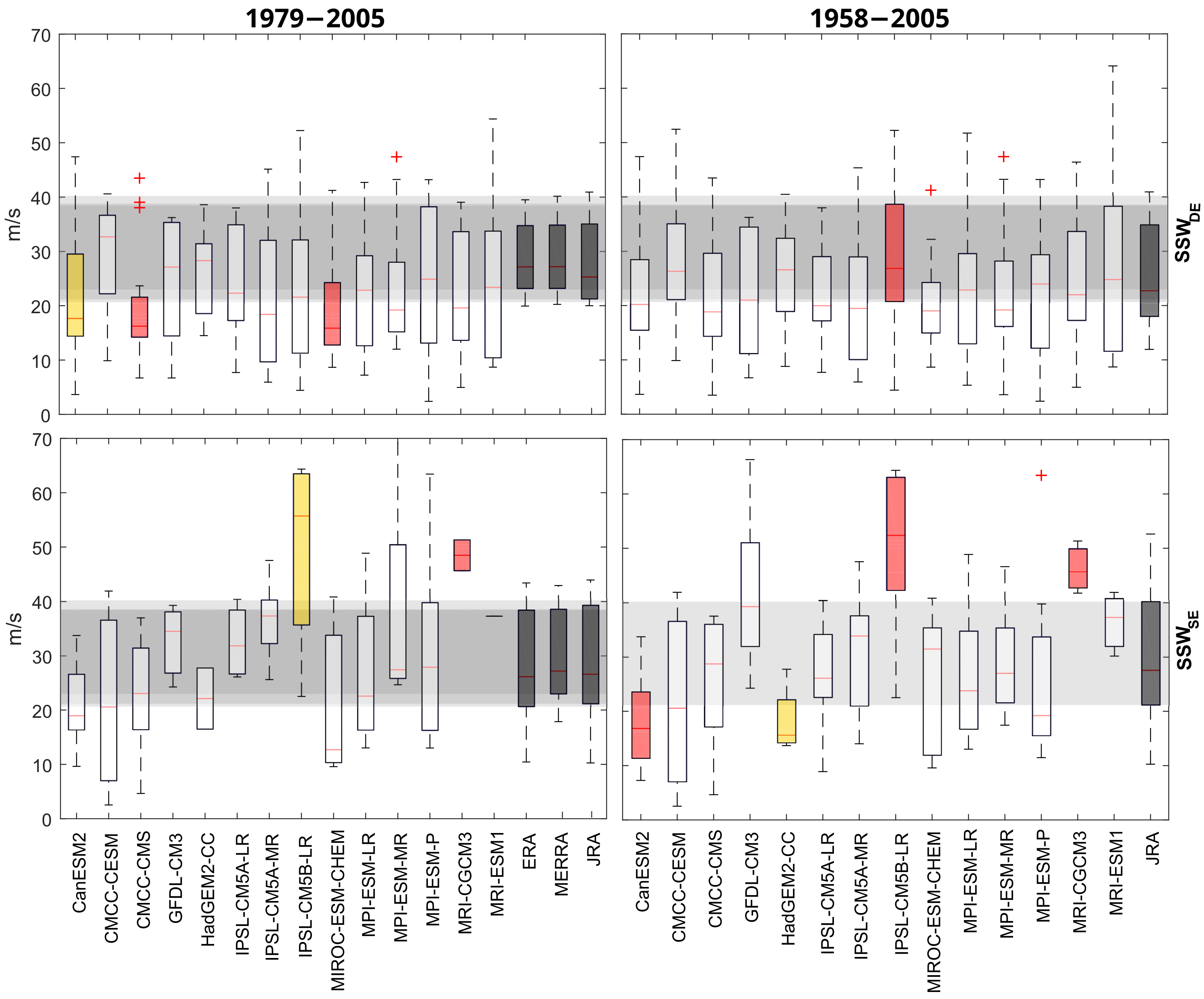
3.4. Polar Vortex Deceleration

The deceleration of the polar stratospheric jet ($\Delta U_{10}$) is defined as the difference in the zonal-mean zonal wind at 60° N and 10 hPa, calculated between the average from 15 to 5 days before the central date of the event and the average from 0 to 5 days after. Figure 3 shows the $\Delta U_{10}$ values obtained from the reanalysis datasets and climate models for $SS{W}_D$ events, considering both the 1979–2005 and 1958–2005 periods. During the satellite era (1979–2005), the CanESM2, CMCC-CMS, and MIROC-ESM-CHEM models show deceleration values significantly different from those in the reanalyses. For the longer period (1958–2005), only the IPSL-CM5B-LR model exhibits statistically significant differences.

For $SS{W}_S$ events, the IPSL-CM5B-LR and MRI-CGCM3 models differ significantly from the reanalyses in both periods, while the CanESM2 and HadGEM2-CC models do so only during the 1958–2005 period.

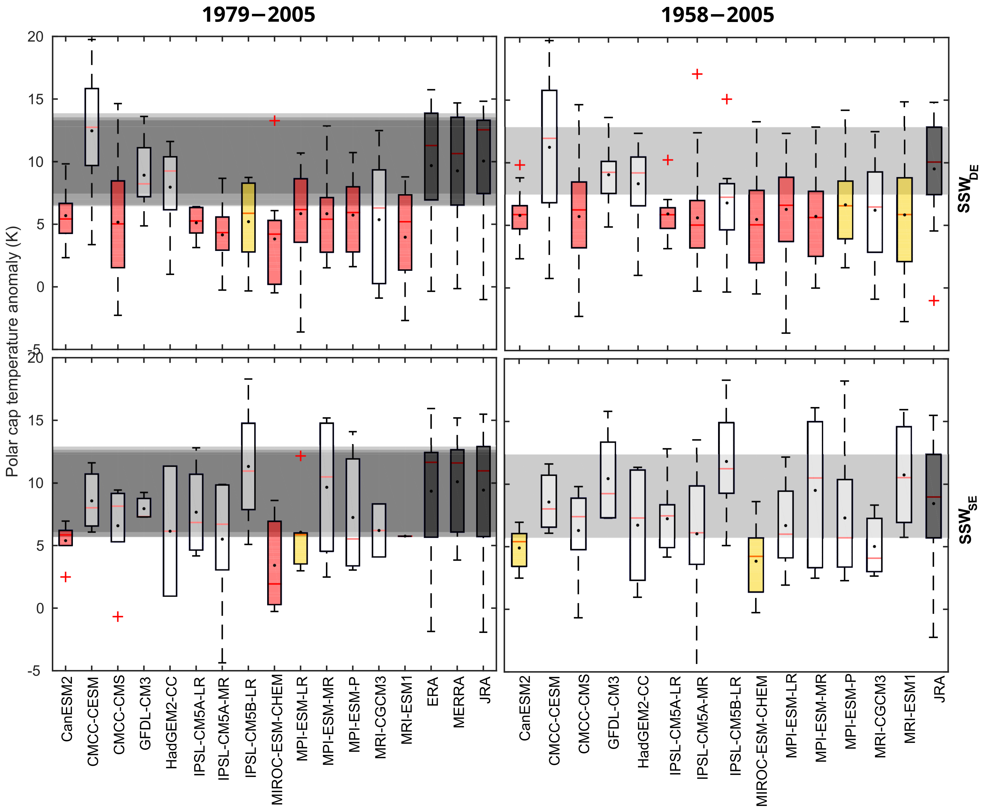
3.5. Polar Cap Temperature

Temperature anomalies over the polar cap are computed at the 10 hPa ($T_{10}^{\prime }$) and 100 hPa ($T_{100}^{\prime }$) levels, averaged between 60° N and 90° N. These are calculated within a ±5-day window around the central date of each event, using an extended temporal range from 40 days before to 80 days after the onset. Figure 4 shows the distribution of $T_{10}^{\prime }$ anomalies for models and reanalyses. For $SS{W}_D$ events, the CMCC-CESM, GFDL-CM3, HadGEM2-CC, and MRI-CGCM3 models show no statistically significant differences from the reanalyses in either period, while IPSL-CM5A-LR is consistent only during the 1979–2005 period. For $SS{W}_S$ events, model performance is improved: only CanESM2 and MIROC-ESM-CHEM differ significantly in both periods, and MPI-ESM-P in the 1979–2005 period.

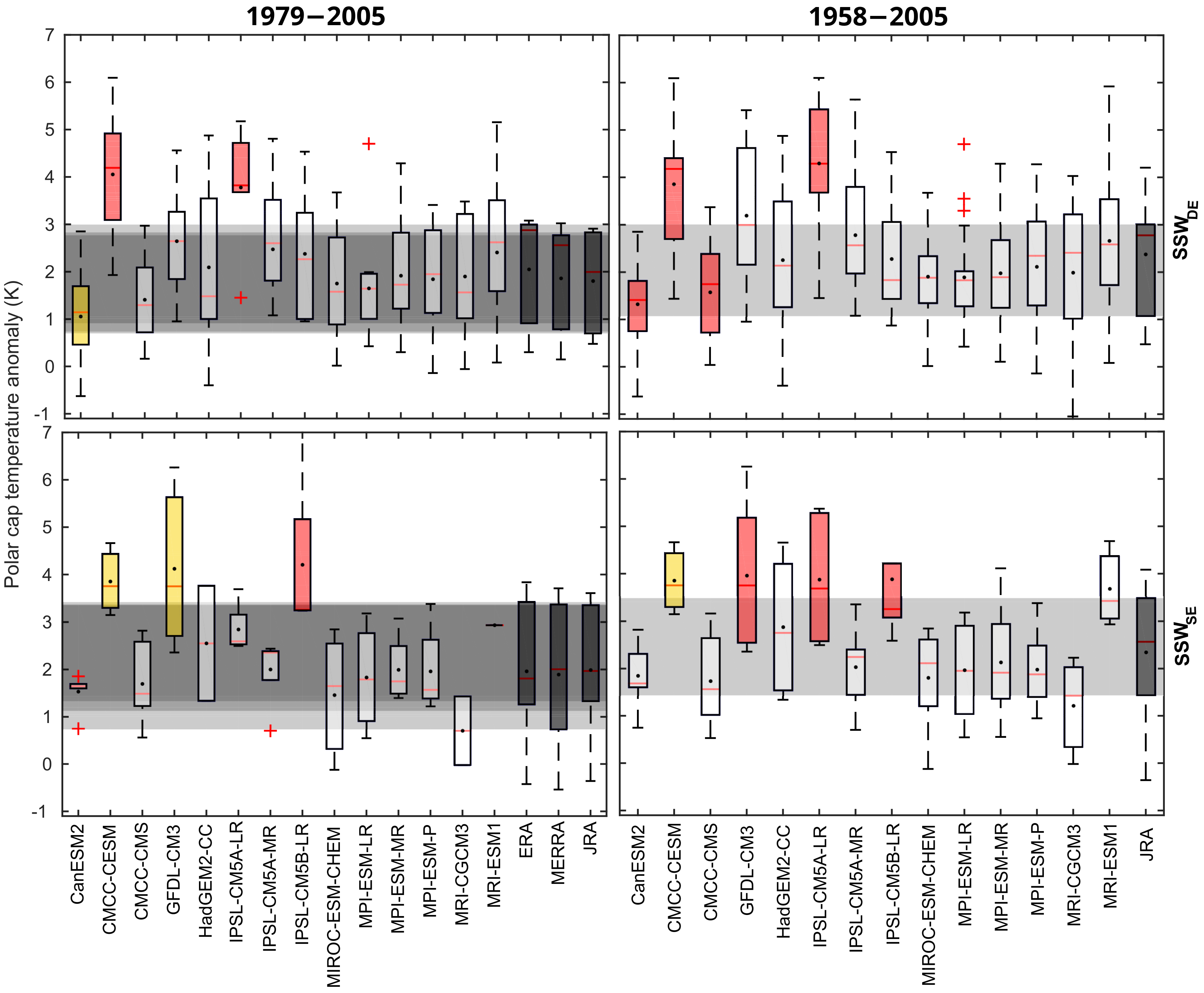
As for the $T_{100}^{\prime }$ anomalies, shown in Figure 5, during $SS{W}_D$ events, the CanESM2, CMCC-CESM, and IPSL-CM5A-LR models deviated significantly from the reanalyses in both periods, while CMCC-CMS shows differences only in the 1958–2005 period. For $SS{W}_S$ events, the CMCC-CESM, GFDL-CM3, and IPSL-CM5B-LR models differ significantly in both periods; CanESM2 only during 1979–2005, and IPSL-CM5A-LR only during 1958–2005.

The results show considerable variability depending on the validation period, as summarized in

Table 4. Summary of the statistical consistency of each model with reanalyses during the 1979–2005 and 1958–2005 periods. Each cell reports a pair of results (A/B), where A corresponds to the 95% confidence level (p > 0.05), and B to the 90% level (p > 0.10). “N” indicates that no statistically significant difference is found between the model and the reanalysis at that level (i.e., p-value exceeds the threshold), while “Y” indicates that the difference is statistically significant (i.e., p-value does not exceed the threshold). The Total column reports how many variables meet the non-significance criterion at each threshold.

	Model	SSW/Winter	${\mathbf{SSW}}_{\mathit{D}}/{\mathbf{SSW}}_{\mathit{S}}$	Duration (${\mathbf{SSW}}_{\mathit{D}}$)	Duration (${\mathbf{SSW}}_{\mathit{S}}$)	Desaceleración (${\mathbf{SSW}}_{\mathit{D}}$)	Desaceleración (${\mathbf{SSW}}_{\mathit{S}}$)	${\overline{{\mathit{T}}^{\prime }}}_{10}$ (${\mathbf{SSW}}_{\mathit{D}}$)	${\overline{{\mathit{T}}^{\prime }}}_{10}$ (${\mathbf{SSW}}_{\mathit{S}}$)	${\overline{{\mathit{T}}^{\prime }}}_{100}$ (${\mathbf{SSW}}_{\mathit{D}}$)	${\overline{{\mathit{T}}^{\prime }}}_{100}$ (${\mathbf{SSW}}_{\mathit{S}}$)	Total
1979–2005.
1	CanESM2	Y/Y	Y/N	N/N	N/N	Y/Y	N/N	Y/N	Y/N	Y/Y	N/N	4/7
2	CMCC-CESM	N/N	N/N	N/N	N/N	N/N	N/N	N/N	N/N	Y/N	Y/Y	8/9
3	CMCC-CMS	N/N	Y/Y	N/N	N/N	Y/N	N/N	Y/N	N/N	N/N	N/N	7/9
4	GFDL-CM3	Y/N	N/N	N/N	N/N	N/N	N/N	N/N	N/N	N/N	Y/Y	8/9
5	HadGEM2-CC	Y/Y	Y/N	N/N	N/N	N/N	N/N	N/N	N/N	N/N	N/N	8/9
6	IPSL-CM5A-LR	Y/N	N/N	N/N	N/N	N/N	N/N	Y/N	N/N	Y/N	N/N	7/10
7	IPSL-CM5A-MR	N/N	N/N	N/N	N/N	N/N	N/N	Y/N	N/N	N/N	N/N	9/10
8	IPSL-CM5B-LR	Y/N	N/N	N/N	Y/Y	N/N	Y/Y	Y/N	N/N	Y/N	N/N	5/8
9	MIROC-ESM-CHEM	N/N	Y/Y	N/N	N/N	Y/N	N/N	Y/N	Y/N	N/N	N/N	6/9
10	MPI-ESM-LR	N/N	Y/Y	N/N	N/N	N/N	N/N	Y/N	Y/Y	N/N	N/N	7/8
11	MPI-ESM-MR	N/N	Y/N	N/N	N/N	N/N	N/N	Y/N	N/N	N/N	N/N	8/10
12	MPI-ESM-P	N/N	N/N	N/N	N/N	N/N	N/N	Y/N	N/N	N/N	N/N	9/10
13	MRI-CGCM3	Y/N	N/N	N/N	N/N	N/N	Y/N	N/N	N/N	N/N	N/N	8/10
14	MRI-ESM1	Y/N	Y/N	N/N	N/N	N/N	N/N	Y/N	N/N	N/N	N/N	7/10
1958–2005
1	CanESM2	Y/Y	Y/N	N/N	Y/Y	N/N	Y/N	Y/N	Y/N	Y/N	N/N	3/8
2	CMCC-CESM	N/N	N/N	Y/Y	N/N	N/N	N/N	N/N	N/N	Y/N	Y/Y	7/8
3	CMCC-CMS	N/N	Y/N	N/N	N/N	N/N	N/N	Y/N	N/N	Y/N	N/N	7/10
4	GFDL-CM3	Y/N	N/N	N/N	Y/N	N/N	N/N	N/N	N/N	N/N	Y/N	7/10
5	HadGEM2-CC	N/N	Y/N	N/N	N/N	N/N	Y/Y	N/N	N/N	N/N	N/N	8/9
6	IPSL-CM5A-LR	Y/Y	N/N	N/N	N/N	N/N	N/N	Y/N	N/N	Y/N	Y/N	6/9
7	IPSL-CM5A-MR	N/N	Y/Y	N/N	N/N	N/N	N/N	Y/N	N/N	N/N	N/N	8/9
8	IPSL-CM5B-LR	Y/N	N/N	N/N	Y/N	Y/N	Y/N	Y/Y	N/N	N/N	Y/N	4/9
9	MIROC-ESM-CHEM	N/N	Y/Y	N/N	Y/N	N/N	N/N	Y/N	Y/N	N/N	N/N	6/9
10	MPI-ESM-LR	N/N	Y/Y	N/N	Y/Y	N/N	N/N	Y/N	Y/Y	N/N	N/N	6/7
11	MPI-ESM-MR	N/N	Y/N	N/N	Y/Y	N/N	N/N	Y/N	N/N	N/N	N/N	7/9
12	MPI-ESM-P	N/N	N/N	N/N	N/N	N/N	N/N	Y/N	N/N	N/N	N/N	9/10
13	MRI-CGCM3	Y/N	N/N	N/N	N/N	N/N	Y/N	N/N	N/N	N/N	N/N	8/10
14	MRI-ESM1	Y/Y	Y/N	N/N	N/N	N/N	N/N	Y/N	N/N	N/N	N/N	7/9

. This variability may reflect not only the intrinsic fluctuations of SSWm but also differences in reanalysis quality, particularly in the pre-satellite era.

4. Discussion

The accuracy of SSWm diagnostics during the pre-satellite period remains subject to greater uncertainty due to the limited and uneven spatial coverage of observations assimilated into reanalysis products [29,30]. Although high-top CMIP5 models are known to improve the representation of stratospheric processes, several exhibit persistent biases in polar vortex climatology, planetary wave propagation, or vertical resolution. These limitations can affect both the frequency and classification of SSWm events [6,12,26].

Our results show that CMIP5 model performance is highly sensitive to the selected validation period and reanalysis dataset. Most models achieved stronger statistical agreement with the reanalyses during the satellite era (1979–2005), whereas model consistency generally declines over the extended historical period (1958–2005), likely reflecting increased observational uncertainty prior to the satellite assimilation era.

A systematic feature across models is the overrepresentation of displacement-type events ($SS{W}_D$) relative to split-type events ($SS{W}_S$), which contrasts with their observed frequency in reanalyses. This bias may reflect shortcomings in the simulated representation of wave–mean flow interactions, particularly in terms of wave-1 and wave-2 dynamics or insufficient vertical resolution.

In this study, SSWm classification is conducted via visual inspection of geopotential height fields following established procedures. While widely accepted, this method introduces a degree of subjectivity. The adoption of automated classification algorithms in future work would enhance the objectivity and reproducibility of results.

Finally, this comparative analysis provides a methodological framework for evaluating SSWm behavior in climate models. The approach is extensible to CMIP6 simulations and to newer generations of reanalyses, including ERA5, MERRA-2, and JRA-3Q, which offer improved resolution, advanced data assimilation schemes, and longer temporal coverage. The results underscore the need to incorporate both dynamical and morphological diagnostics when assessing stratospheric model fidelity.

5. Conclusions

This study assessed the ability of 14 CMIP5 climate models to simulate SSWm, using five key metrics: event frequency, morphological classification, duration, polar jet deceleration, and polar temperature anomalies. Validation was conducted against three reanalysis datasets over two periods: the satellite era (1979–2005), and a longer historical period including pre-satellite years (1958–2005).

Results indicate that model performance depends strongly on the selected validation period. Improved agreement with reanalyses is generally observed during the satellite period, likely due to the higher reliability of reanalysis products under dense observational coverage. For instance, based on the consistency scores across all metrics, six models showed better agreement with reanalyses during the 1979–2005 period under the p > 0.10 threshold, while three models worsened, and five remained unchanged. Under the more relaxed p > 0.05 criterion, eight models improved, and six showed no change. These findings emphasize the importance of using multiple periods and significance thresholds in SSWm model evaluation and reinforce the value of satellite-era data for robust validation.

A group of seven models (CMCC-CESM, GFDL-CM3, HadGEM2-CC, IPSL-CM5A-MR, MPI-ESM-MR, MPI-ESM-P, and MRI-CGCM3) demonstrated high consistency with reanalysis during the satellite era, showing no statistically significant differences (p > 0.05) in at least eight of the ten metrics. Notably, CMCC-CESM, IPSL-CM5A-MR, and MPI-ESM-P performed robustly across both event frequency and classification. In contrast, CanESM2 and IPSL-CM5B-LR exhibited lower agreement, particularly during the extended period. These patterns support the prioritization of well-performing models and highlight the sensitivity of model validation outcomes to the chosen time window and diagnostic metric.

The systematic overrepresentation of $SS{W}_D$ events in models, as opposed to the observed dominance of $SS{W}_S$ events in reanalyses, further underscores the importance of incorporating event morphology in evaluation frameworks. Morphology-based classification provides essential complementary information beyond dynamical metrics alone.

Overall, this study contributes a robust framework for assessing the representation of SSWm events in climate models. The findings are directly applicable to future model intercomparison projects and validation efforts involving CMIP6 models and next-generation reanalysis datasets such as ERA5, MERRA-2, and JRA-3Q.

References

- Gimeno, L.; de la Torre, L.; Nieto, R.; Gallego, D.; Ribera, P.; García-Herrera, R. A new diagnostic of stratospheric polar vortices. J. Atmos. Sol. Terr. Phys. 2007, 69, 1797–1812. [Google Scholar] [CrossRef]
- Liberato, M.L.R.; Castanheira, J.M.; de la Torre, L.; DaCamara, C.C.; Gimeno, L. Wave Energy Associated with the Variability of the Stratospheric Polar Vortex. J. Atmos. Sci. 2007, 64, 2683–2694. [Google Scholar] [CrossRef]
- Castanheira, J.M.; Liberato, M.L.R.; de la Torre, L.; Graf, H.F.; DaCamara, C.C. Baroclinic Rossby Wave Forcing and Barotropic Rossby Wave Response to Stratospheric Vortex Variability. J. Atmos. Sci. 2009, 66, 902–914. [Google Scholar] [CrossRef]
- Waugh, D.W.; Sobel, A.H.; Polvani, L.M. What Is the Polar Vortex and How Does It Influence Weather? Bull. Amer. Meteorol. Soc. 2017, 98, 37–44. [Google Scholar] [CrossRef]
- Mitchell, D.M.; Scott, R.K.; Seviour, W.J.M.; Thomson, S.I.; Waugh, D.W.; Teanby, N.A.; Ball, E.R. Polar Vortices in Planetary Atmospheres. Rev. Geophys. 2021, 59, e2020RG000723. [Google Scholar] [CrossRef]
- Charlton, A.J.; Polvani, L.M.; Perlwitz, J.; Sassi, F.; Manzini, E.; Shibata, K.; Pawson, S.; Nielsen, J.E.; Rind, D. A New Look at Stratospheric Sudden Warmings. Part II: Evaluation of Numerical Model Simulations. J. Clim. 2007, 20, 470–488. [Google Scholar] [CrossRef]
- Shepherd, T.G. Issues in Stratosphere-troposphere Coupling. J. Meteorol. Soc. Jpn. Ser. II 2002, 80, 769–792. [Google Scholar] [CrossRef]
- de la Torre, L.; Garcia, R.R.; Barriopedro, D.; Chandran, A. Climatology and characteristics of stratospheric sudden warmings in the Whole Atmosphere Community Climate Model. J. Geophys. Res. Atmos. 2012, 117, D04110. [Google Scholar] [CrossRef]
- Añel, J.A. The stratosphere: History and future a century after its discovery. Contemp. Phys. 2016, 57, 230–233. [Google Scholar] [CrossRef]
- Chandran, A.; Collins, R.L.; Garcia, R.R.; Marsh, D.R.; Harvey, V.L.; Yue, J.; de la Torre, L. A climatology of elevated stratopause events in the whole atmosphere community climate model. J. Geophys. Res. Atmos. 2013, 118, 1234–1246. [Google Scholar] [CrossRef]
- Baldwin, M.P.; Ayarzagüena, B.; Birner, T.; Butchart, N.; Butler, A.H.; Charlton-Perez, A.J.; Domeisen, D.I.V.; Garfinkel, C.I.; Garny, H.; Gerber, E.P.; et al. Sudden Stratospheric Warmings. Rev. Geophys. 2021, 59, e2020RG000708. [Google Scholar] [CrossRef]
- Charlton-Perez, A.J.; Baldwin, M.P.; Birner, T.; Black, R.X.; Butler, A.H.; Calvo, N.; Davis, N.A.; Gerber, E.P.; Gillett, N.; Hardiman, S.; et al. On the lack of stratospheric dynamical variability in low-top versions of the CMIP5 models. J. Geophys. Res. Atmos. 2013, 118, 2494–2505. [Google Scholar] [CrossRef]
- Osprey, S.M.; Gray, L.J.; Hardiman, S.C.; Butchart, N.; Hinton, T.J. Stratospheric Variability in Twentieth-Century CMIP5 Simulations of the Met Office Climate Model: High Top versus Low Top. J. Clim. 2013, 26, 1595–1606. [Google Scholar] [CrossRef]
- Seviour, W.J.M.; Gray, L.J.; Mitchell, D.M. Stratospheric polar vortex splits and displacements in the high-top CMIP5 climate models. J. Geophys. Res. Atmos. 2016, 121, 1400–1413. [Google Scholar] [CrossRef]
- Lehtonen, I.; Karpechko, A.Y. Observed and modeled tropospheric cold anomalies associated with sudden stratospheric warmings. J. Geophys. Res. Atmos. 2016, 121, 1591–1610. [Google Scholar] [CrossRef]
- Kim, J.; Son, S.W.; Gerber, E.P.; Park, H.S. Defining Sudden Stratospheric Warming in Climate Models: Accounting for Biases in Model Climatologies. J. Clim. 2017, 30, 5529–5546. [Google Scholar] [CrossRef]
- Taguchi, M. A study of different frequencies of major stratospheric sudden warmings in CMIP5 historical simulations. J. Geophys. Res. Atmos. 2017, 122, 5144–5156. [Google Scholar] [CrossRef]
- Ayarzagüena, B.; Polvani, L.M.; Langematz, U.; Akiyoshi, H.; Bekki, S.; Butchart, N.; Dameris, M.; Deushi, M.; Hardiman, S.C.; Jöckel, P.; et al. No Robust Evidence of Future Changes in Major Stratospheric Sudden Warmings: A Multi-model Assessment from CCMI. Chem. Phys. Discuss. 2018, 2018, 11277–11287. [Google Scholar] [CrossRef]
- Wu, Z.; Reichler, T. Variations in the Frequency of Stratospheric Sudden Warmings in CMIP5 and CMIP6 and Possible Causes. J. Climate 2020, 33, 10305–10320. [Google Scholar] [CrossRef]
- Matsuno, T. A Dynamical Model of the Stratospheric Sudden Warming. J. Atmos. Sci. 1971, 28, 1479–1494. [Google Scholar] [CrossRef]
- Andrews, D.G.; Holton, J.R.; Leovy, C.B. Middle Atmosphere Dynamics; Andrews, D.G., Holton, J.R., Leovy, C.B., Eds.; Academic Press: Orlando, FL, USA, 1987; pp. xi–489. [Google Scholar]
- Castanheira, J.M.; Barriopedro, D. Dynamical connection between tropospheric blockings and stratospheric polar vortex. Geophys. Res. Lett. 2010, 37. [Google Scholar] [CrossRef]
- Limpasuvan, V.; Richter, J.H.; Orsolini, Y.J.; Stordal, F.; Kvissel, O.K. The roles of planetary and gravity waves during a major stratospheric sudden warming as characterized in WACCM. J. Atmos. Sol. Terr. Phys. 2012, 78–79, 84–98, Structure and Dynamics of Mesosphere and Lower Thermosphere. [Google Scholar] [CrossRef]
- Sassi, F.; Liu, H.L. Westward traveling planetary wave events in the lower thermosphere during solar minimum conditions simulated by SD-WACCM-X. J. Atmos. Sol. Terr. Phys. 2014, 119, 11–26. [Google Scholar] [CrossRef]
- Huang, J.; Tian, W.; Gray, L.J.; Zhang, J.; Li, Y.; Luo, J.; Tian, H. Preconditioning of Arctic Stratospheric Polar Vortex Shift Events. J. Clim. 2018, 31, 5417–5436. [Google Scholar] [CrossRef]
- Hall, R.J.; Mitchell, D.M.; Seviour, W.J.M.; Wright, C.J. Persistent Model Biases in the CMIP6 Representation of Stratospheric Polar Vortex Variability. J. Geophys. Res. Atmos. 2021, 126, e2021JD034759. [Google Scholar] [CrossRef]
- Chávez, V.M.; Añel, J.A.; Garcia, R.R.; Šácha, P.; Torre, L.d.l. Impact of Increased Vertical Resolution in WACCM on the Climatology of Major Sudden Stratospheric Warmings. Atmosphere 2022, 13, 546. [Google Scholar] [CrossRef]
- Rao, J.; Garfinkel, C.I. CMIP5/6 models project little change in the statistical characteristics of sudden stratospheric warmings in the 21st century. Environ. Res. Lett. 2021, 16, 034024. [Google Scholar] [CrossRef]
- Hitchcock, P. On the value of reanalyses prior to 1979 for dynamical studies of stratosphere–troposphere coupling. Atmos. Chem. Phys. 2019, 19, 2749–2764. [Google Scholar] [CrossRef]
- Gerber, E.P.; Martineau, P. Quantifying the variability of the annular modes: Reanalysis uncertainty vs. sampling uncertainty. Atmos. Chem. Phys. 2018, 18, 17099–17117. [Google Scholar] [CrossRef]
- Fujiwara, M.; Wright, J.S.; Manney, G.L.; Gray, L.J.; Anstey, J.; Birner, T.; Davis, S.; Gerber, E.P.; Harvey, V.L.; Hegglin, M.I.; et al. Introduction to the SPARC Reanalysis Intercomparison Project (S-RIP) and overview of the reanalysis systems. Atmos. Chem. Phys. 2017, 17, 1417–1452. [Google Scholar] [CrossRef]
- Dell’Aquila, A.; Lucarini, V.; Ruti, P.; Calmanti, S. Hayashi Spectra of the Northern Hemisphere Mid-latitude Atmospheric Variability in the NCEP and ERA 40 Reanalyses. arXiv 2004, arXiv:0412150. [Google Scholar] [CrossRef]
- Kobayashi, C.; Endo, H.; Ota, Y.; Kobayashi, S.; Onoda, H.; Harada, Y.; Onogi, K.; Kamahori, H. Preliminary Results of the JRA-55C, an Atmospheric Reanalysis Assimilating Conventional Observations Only. SOLA 2014, 10, 78–82. [Google Scholar] [CrossRef]
- Bell, B.; Hersbach, H.; Simmons, A.; Berrisford, P.; Dahlgren, P.; Horányi, A.; Muñoz-Sabater, J.; Nicolas, J.; Radu, R.; Schepers, D.; et al. The ERA5 global reanalysis: Preliminary extension to 1950. Quart. J. Roy. Meteorol. Soc. 2021, 147, 4186–4227. [Google Scholar] [CrossRef]
- Serva, F.; Christiansen, B.; Davini, P.; von Hardenberg, J.; van den Oord, G.; Reerink, T.J.; Wyser, K.; Yang, S. Changes in Stratospheric Dynamics Simulated by the EC-Earth Model From CMIP5 to CMIP6. J. Adv. Model. Earth Syst. 2024, 16, e2023MS003756. [Google Scholar] [CrossRef]
- Manzini, E.; Karpechko, A.Y.; Anstey, J.; Baldwin, M.P.; Black, R.X.; Cagnazzo, C.; Calvo, N.; Charlton-Perez, A.; Christiansen, B.; Davini, P.; et al. Northern winter climate change: Assessment of uncertainty in CMIP5 projections related to stratosphere-troposphere coupling. J. Geophys. Res. Atmos. 2014, 119, 7979–7998. [Google Scholar] [CrossRef]
- Lott, F.; Denvil, S.; Butchart, N.; Cagnazzo, C.; Giorgetta, M.A.; Hardiman, S.C.; Manzini, E.; Krismer, T.; Duvel, J.; Maury, P.; et al. Kelvin and Rossby-gravity wave packets in the lower stratosphere of some high-top CMIP5 models. J. Geophys. Res. Atmos. 2002, 119, 2156–2173. [Google Scholar] [CrossRef]
- Dee, D.P.; Uppala, S.M.; Simmons, A.J.; Berrisford, P.; Poli, P.; Kobayashi, S.; Andrae, U.; Balmaseda, M.A.; Balsamo, G.; Bauer, P.; et al. The ERA-Interim reanalysis: Configuration and performance of the data assimilation system. Q. J. Royal Meteorol. Soc. 2011, 137, 553–597. [Google Scholar] [CrossRef]
- Rienecker, M.M.; Suarez, M.J.; Gelaro, R.; Todling, R.; Bacmeister, J.; Liu, E.; Bosilovich, M.G.; Schubert, S.D.; Takacs, L.; Kim, G.K.; et al. MERRA: NASA’s Modern-Era Retrospective Analysis for Research and Applications. J. Clim. 2011, 24, 3624–3648. [Google Scholar] [CrossRef]
- Ebita, A.; Kobayashi, S.; Ota, Y.; Moriya, M.; Kumabe, R.; Onogi, K.; Harada, Y.; Yasui, S.; Miyaoka, K.; Takahashi, K.; et al. The Japanese 55-year Reanalysis “JRA-55”: An interim report. SOLA 2011, 7, 149–152. [Google Scholar] [CrossRef]
- KobayashiI, S.; Ota, Y.; Harada, Y.; Ebita, A.; Moriya, M.; Onoda, H.; Onogi, K.; Kamahori, H.; Kobayashi, C.; Endo, H.; et al. The JRA-55 Reanalysis: General Specifications and Basic Characteristics. J. Meteor. Soc. Japan 2015, 93, 5–48. [Google Scholar] [CrossRef]
- Charlton, A.J.; Polvani, L.M. A New Look at Stratospheric Sudden Warmings. Part I: Climatology and Modeling Benchmarks. J. Clim. 2007, 20, 449–469. [Google Scholar] [CrossRef]
- World Meteorological Organization/IQSY. International Years of the Quiet Sun (IQSY) 1964-65. Alert Messages with Special References to Stratwarms; WMO/IQSY Report No 6. Technical Report; World Meteorological Organization: Geneva, Switzerland, 1964. [Google Scholar]