Deep Learning-Based Vertical Decomposition of Ionospheric TEC into Layered Electron Density Profiles

Abstract

This study proposes a deep learning-based vertical decomposition model for ionospheric Total Electron Content (TEC), which establishes a nonlinear mapping from macroscale TEC data to vertically layered electron density (Ne) spanning 60–800 km by integrating geomagnetic indices (AE, SYM-H) and solar activity parameters (F10.7). Utilizing global TEC grid data (spatiotemporal resolution: 1 h/5.625° × 2.8125°) provided by the International GNSS Service (IGS), a Multilayer Perceptron (MLP) model was developed, taking spatiotemporal coordinates, altitude, and space environment parameters as inputs to predict logarithmic electron density ln(Ne). Experimental validation against COSMIC-2 radio occultation observations in 2019 demonstrates the model’s capability to capture ionospheric vertical structures, with a prediction performance significantly outperforming the International Reference Ionosphere model IRI-2020: root mean square error (RMSE) decreased by 34.16%, and the coefficient of determination (R²) increased by 28.45%. This method overcomes the reliance of traditional electron density inversion on costly radar or satellite observations, enabling high-spatiotemporal-resolution global ionospheric profile reconstruction using widely available GNSS-TEC data. It provides a novel tool for space weather warning and shortwave communication optimization. Current limitations include insufficient physical interpretability and prediction uncertainty in GNSS-sparse regions, which could be mitigated in future work through the integration of physical constraints and multi-source data assimilation.

1. Introduction

Total Electron Content (TEC), defined as the integrated electron count within a vertical column of unit cross-sectional area along a signal propagation path (unit: TECU, 1 TECU = 10¹⁶ electrons/m²), characterizes the horizontal distribution of ionospheric electron content and serves as a path-integrated parameter describing the macroscopic state of the ionosphere [1]. Compared to macroscale TEC, electron density (Ne), a microscopic parameter quantifying local ionization levels (unit: electrons/m³), precisely delineates the fine vertical structural characteristics of the ionosphere by revealing altitude-dependent stratification (e.g., D, E, and F layers) and diurnal ionization variations (e.g., nocturnal F-layer density decay) [2]. In recent years, efforts in TEC-to-Ne modeling have focused on developing data-driven approaches. For instance, studies have utilized GNSS-TEC data to optimize ionospheric models like the International Reference Ionosphere (IRI-2016) for more accurate electron density profile estimations [3].

As a macroscopic observable factor, TEC holds critical operational value in space weather services. In satellite navigation, real-time TEC monitoring provides ionospheric delay correction parameters for GNSS systems. For instance, abrupt global TEC enhancements during geomagnetic storms can amplify GPS positioning errors to tens of meters [4], while TEC anomaly-based early warnings effectively mitigate ionospheric disturbances caused by solar events (e.g., solar flares, coronal mass ejections) in navigation and communication systems [5]. In comparison, the vertical distribution of Ne carries greater physical significance for radio wave propagation: Electron density gradients directly govern radio wave refraction paths and propagation losses. For example, shortwave communication systems require dynamic selection of optimal operating frequencies based on Ne peaks in the E-layer (90–150 km) and F-layer (>150 km) to avoid signal attenuation [6].

TEC and Ne describe ionospheric characteristics through two distinct dimensions: path-integrated quantities and spatial gradients, respectively. Their synergistic study forms the foundation of ionospheric multi-scale modeling; while TEC provides critical input parameters for Global Navigation Satellite Systems (GNSS) and space weather monitoring, Ne underpins research on ionospheric dynamic mechanisms and the optimization of communication systems. Consequently, achieving joint inversion of TEC and Ne constitutes a central challenge in enhancing the spatiotemporal precision of ionospheric models. Traditional physics-based approaches have also analyzed electron density gradients by investigating their mapping relationships [7].

However, the current vertical profiling of electron density faces significant technological bottlenecks: While incoherent scatter radar (ISR) can provide high-precision Ne profile data, its exorbitant single-station deployment costs and sparse global coverage [8,9,10] limit its widespread application. Conversely, GNSS radio occultation techniques using low-Earth-orbit satellites (e.g., COSMIC-2) achieve global coverage but are characterized by specific spatial resolution limitations. COSMIC-2 electron density profiles typically have a vertical resolution of about 0.5 km and a horizontal resolution of about 200 km. Although the mission provides approximately 5000 soundings per day with high density, these spatial limitations, primarily imposed by orbital parameters and the radio occultation technique itself, can still hinder their ability to fully capture rapid transient processes or small-scale structures of ionospheric parameters [11,12,13]. By comparison, ground-based GNSS-TEC observation networks have attained global continuous monitoring capabilities with high spatiotemporal resolution [1,14,15,16].

Against this backdrop, electron density inversion methods based on global ionospheric TEC grid products (e.g., IGS-TEC) demonstrate unique application advantages. First, by constructing cross-scale TEC-Ne mapping relationships through deep learning, these methods transform widely available TEC data into finely resolved vertical profile information, effectively compensating for the spatial coverage limitations of traditional observation techniques. Second, the high-resolution Ne data obtained from inversion serve dual purposes: acting as data assimilation sources for ISR and occultation observations, while also providing validation benchmarks for first-principles-based ionospheric numerical models. This technical approach—leveraging easily accessible parameters to infer difficult-to-measure ones—delivers an innovative solution to overcome ionospheric vertical structure monitoring bottlenecks. Furthermore, the rapid advancement of deep learning has spurred significant progress in ionospheric modeling, particularly in developing high-precision TEC prediction models [17,18,19,20]. Studies in this area have demonstrated the effectiveness of deep learning architectures, often utilizing Recurrent Neural Networks like LSTM and incorporating diverse training data including historical TEC and indices of solar and geomagnetic activity, to forecast TEC with improved accuracy. Building upon these advancements in leveraging deep learning for ionospheric data analysis, our study applies these data-driven techniques to a complementary problem: establishing TEC-to-Ne inversion relationships. While TEC prediction focuses on forecasting future conditions [17,18,19,20], our approach leverages widely available instantaneous TEC grid products to infer detailed vertical electron density profiles, offering a distinct but related application and highlighting the broad potential of deep learning in ionospheric characterization.

This study proposes a deep learning-based Ionospheric Vertical Decomposition Framework (IVDF), which establishes a cross-scale mapping model from macroscale TEC to electron density vertical profiles by integrating IGS-TEC grid data with multi-source space environment parameters (AE, SYM-H, F10.7). The framework aims to rapidly and accurately derive globally distributed vertical electron density through the synergistic use of TEC, geomagnetic indices (AE, SYM-H), solar activity parameters (F10.7), and essential spatiotemporal information. The innovation of IVDF is threefold:

(a)

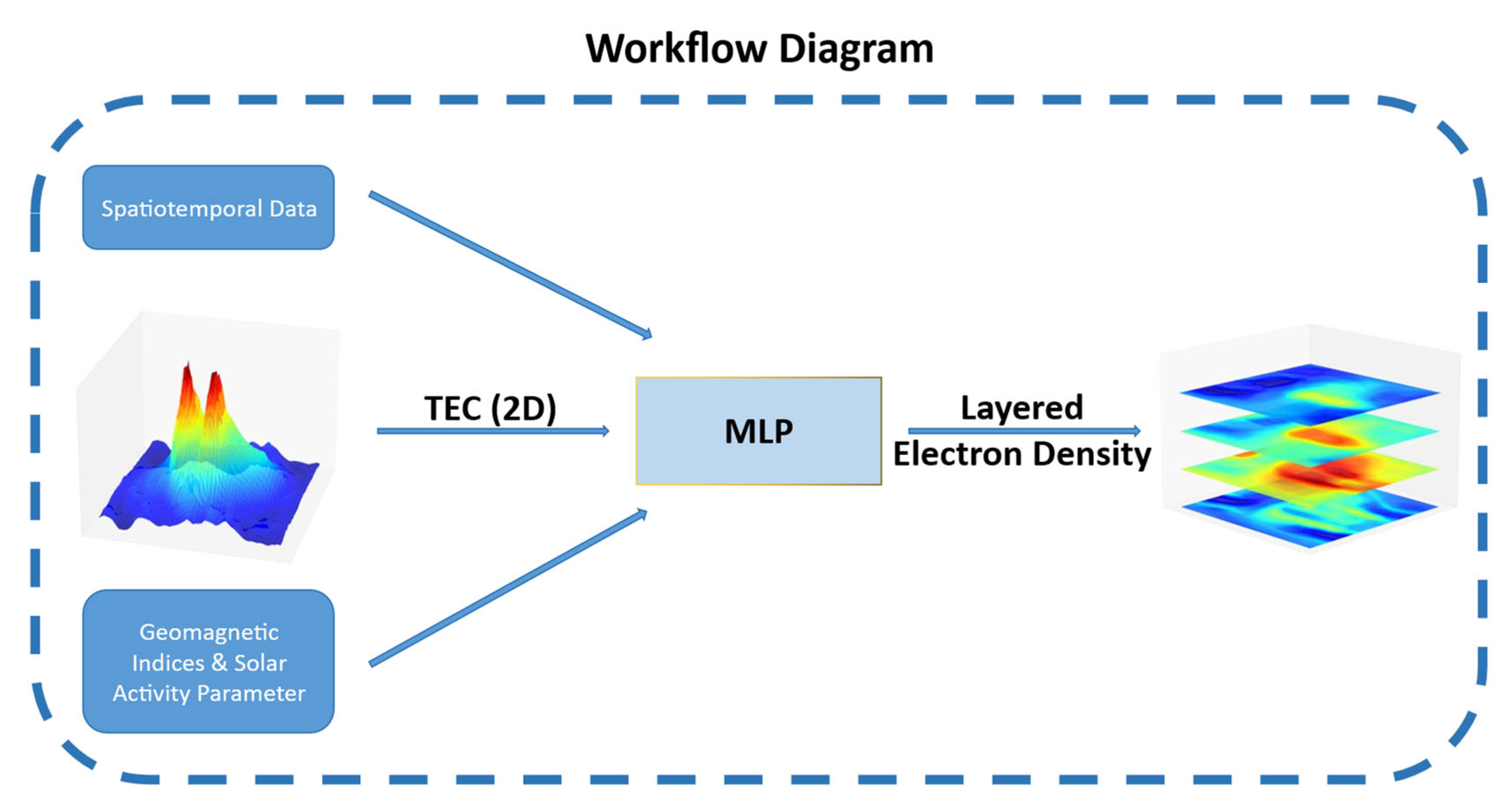
Dynamic Magnetospheric Coupling: Geomagnetic activity indices (AE/SYM-H) are incorporated as dynamic drivers into the deep learning architecture to explicitly characterize the control mechanisms of magnetospheric energy injection on ionospheric Ne abrupt changes.

(b)

Adaptive Spatial Encoding: Longitude periodicity encoding (sine and cosine transformations) and a logarithmic Ne output layer are introduced to enhance the model’s adaptability to ionospheric longitudinal–latitudinal variation patterns and Ne magnitudes spanning multiple orders.

(c)

Full-Profile Real-Time Inversion: A vertically decomposed network covering 60–800 km altitudes enables real-time global Ne profile retrieval using single-input TEC data.

To validate the feasibility of TEC-based vertical decomposition, this study adopts a lightweight Multilayer Perceptron (MLP) model as a proof of concept. While more complex architectures (e.g., CNNs, RNNs, Transformers) could better capture spatiotemporal dependencies, they are reserved for future work aimed at further improving accuracy and generalization.

2. Materials and Methods

2.1. Data Sources and Preprocessing

(a)

IGS-TEC

IGS-TEC (International GNSS Service Total Electron Content) is a global ionospheric Total Electron Content (TEC) product developed and disseminated by the International GNSS Service (IGS). This dataset is generated through multi-frequency signal differential techniques and ionospheric modeling methods, leveraging a globally distributed network of GNSS dual-frequency stations (e.g., GPS, BDS, Galileo). It is designed to deliver high-precision ionospheric parameters in support of navigation, communication, and space weather research.

This study utilizes data from 2011 to 2019 with a temporal resolution of 1 h (UTC). The original TEC data with a grid size of 71 × 73 was processed using bilinear interpolation, resulting in a global grid of 64 × 64 dimensions that maintains a longitudinal resolution of 5.625° and latitudinal resolution of 2.8125°. This method was selected primarily for its computational efficiency and simplicity in regridding existing gridded data, which is a standard approach for this type of preprocessing. While more advanced spatial interpolation techniques such as Kriging or Natural Neighbor Interpolation offer advantages in interpolating scattered data or capturing complex spatial structures, bilinear interpolation was deemed sufficient for this study’s objective of preparing existing gridded TEC data for deep learning inversion [21,22]. Figure 1 illustrates the spatial distribution of TEC. The reconstructed electron density shares an identical spatial resolution with TEC, while its vertical coverage spans 60–800 km with a step size of 10 km, resulting in 75 discrete altitude layers, as shown in Figure 2.

(b)

AE, SYM-H, and F10.7

The AE index quantifies the intensity of auroral electrojet currents by measuring horizontal geomagnetic field disturbances at high latitudes (unit: nanotesla, nT). Its data are derived from synchronized observations by Arctic geomagnetic station chains (e.g., Alaska, Canada, Scandinavia), reflecting energy inputs from ionosphere–magnetosphere coupling processes during substorm activities.

The SYM-H index, calculated as the global average of horizontal magnetic field disturbances from mid- to low-latitude stations, characterizes ring current intensity during geomagnetic storms (unit: nT). The magnitude of its negative values directly correlates with storm severity.

The F10.7 index measures solar radio flux at 10.7 cm wavelength (2.8 GHz) in solar flux units (SFU), serving as a canonical proxy for solar extreme ultraviolet (EUV) radiation intensity and solar activity levels (e.g., sunspot numbers and flare activity). It also serves as a robust indicator of radio wave propagation conditions.

This study employs hourly-level data from these three parameters, temporally and spatially aligned with IGS-TEC records (per-data-point alignment), as input features for ionospheric modeling. AE and SYM-H are incorporated to enable the model to capture magnetospheric energy injection-driven abrupt Ne variations, particularly those affecting the vertical electron density profile. As indicators of substorm (AE) and storm (SYM-H) activity, these indices reflect disturbances in ionospheric electric fields and plasma drifts, which significantly modify the vertical distribution of ionization in the F-layer, altering its shape and peak height. For instance, studies show that substorms (reflected in AE) cause significant disturbances in vertical plasma drift in the F-region [23]. Similarly, observations using Ne retrieval profiles during geomagnetic storms (characterized by significant SYM-H variations) have shown enhancements and uplifting of electron density structures [24], while F10.7 seeks to enable the model to uncover solar radiation’s long-term modulation effects on ionospheric ionization rates.

(c)

COSMIC-1

The COSMIC-1 (Constellation Observing System for Meteorology, Ionosphere, and Climate-1)/FORMOSAT-3 satellite constellation, launched in 2006, pioneered global atmospheric profiling using GNSS radio occultation. Comprising six polar-orbiting satellites (800 km altitude), it delivered over 2500 daily vertical profiles of atmospheric parameters and ionospheric electron density, establishing foundational datasets for numerical weather prediction and space weather studies [25]. In this study, the source of electron density used for training is reconstructed from COSMIC-1 observations.

(d)

COSMIC-2

COSMIC-2 (Constellation Observing System for Meteorology, Ionosphere, and Climate-2) is a second-generation satellite constellation for meteorological, ionospheric, and climate observation, launched in 2019. With the primary objective of acquiring high-precision, high-vertical-resolution atmospheric and ionospheric profile data through GNSS radio occultation techniques, it aims to enhance weather forecasting, space weather monitoring, and climate studies. The constellation comprises six low-inclination orbit satellites, delivering dense observational coverage from tropical to mid-latitude regions (±45°), and providing approximately 5000 daily vertical radio occultation profiles of atmospheric parameters and electron density [26]. This study employs its 2019 electron density (Ne) observations as a benchmark observational dataset to validate the output accuracy of the decomposition model.

The 2019 COSMIC-2 data used in this study were obtained from official sources as raw.tar.gz archive files, whose filenames incorporate the day of the year (DOY). The DOY range for 2019 data spans 274–365. After decompression, each archive yields multiple NetCDF-format files, each containing spatiotemporal metadata (e.g., timestamp, satellite ID) encoded in filenames. Hourly parameters were extracted from filenames, while altitude, latitude, longitude, and electron density (Ne) were retrieved from file contents.

Data cleaning followed three criteria:

• Missing Value Removal: Rows containing placeholder values (−999) were discarded.
• Physical Validity Filtering: Observations with Ne < 0 (non-physical values) were excluded.
• Altitude Thresholding: Data below 60 km were truncated to align with the training data range.

After applying these cleaning criteria to the 2019 COSMIC-2 electron density observations (from DOY 274–365), a total of 38,609,157 valid data points were retained for subsequent modeling.

The cleaned satellite altitude distribution is illustrated in Figure 3.

(e)

IRI-2020

The International Reference Ionosphere (IRI) is an empirical standard model constructed from extensive global ionospheric observational data. By integrating ground-based and satellite observations, it systematically characterizes the global distribution of key ionospheric parameters, including but not limited to electron density (Ne) vertical profiles, ion composition ratios, electron/ion temperatures, and ionospheric drift velocities [27].

This study utilizes electron density (Ne) outputs from IRI-2020 (current latest version) as a comparative reference to evaluate the modeling performance of the data-driven approach through systematic comparisons with predictions from the deep learning model. The IRI-2020 model has improved empirical algorithms and integrated next-generation observational datasets compared to its predecessors, significantly enhancing its capability to characterize ionospheric spatiotemporal variations.

By establishing this comparative validation framework, the study not only enables quantitative evaluation of the deep learning model’s performance in ionospheric parameter inversion but also helps to reveal the complementarity and applicability boundaries between empirical and data-driven models in ionospheric modeling. These outcomes provide theoretical foundations for advancing multi-source ionospheric data fusion and innovative modeling methodologies.

2.2. Deep Learning MLP Methodology

This study developed a deep neural network based on a Multilayer Perceptron (MLP) architecture to achieve nonlinear mapping from macroscale TEC to vertically layered electron density (60–800 km) through the integration of IGS-TEC data, geomagnetic–solar activity parameters, and essential spatiotemporal inputs. Figure 4 illustrates the workflow of the proposed model.

The model inputs comprise nine dimensional features, including hour of the day (integer), latitude (in radians), sine and cosine of longitude (radian units), altitude, AE, SYM-H, and F10.7. Longitude is transformed into trigonometric representations (sine and cosine encoding) to better capture the periodicity of longitude. The output label is electron density in logarithmic units (ln(e/m³)), which effectively compresses the target variable’s dynamic range (spanning multiple orders of magnitude) to mitigate training instability and gradient-vanishing issues. Detailed input–output specifications are provided in

Table 1. Summary of input and output data of decomposition model. The table summarizes the nine input parameters (name and unit) and the single output prediction target (ln(Ne) in ln(m⁻³)).

Feature		Label
Channel Name	Unit	Channel Name	Unit
TEC	TECU	Ne	ln(m−3)
Latitude	rad	-	-
sin(Longitude)	-	-	-
cos(Longitude)	-	-	-
Altitude	km	-	-
AE	nT	-	-
SYM-H	nT	-	-
F10.7	SFU	-	-
Hour	-	-	-

.

The network comprises three fully connected hidden layers with 128, 64, and 32 neurons sequentially, each followed by a ReLU (Rectified Linear Unit) activation function to introduce nonlinear expressiveness:

$$ReLU\left(x\right)=\max \left(0,x\right)$$

(1)

The model employs mean squared error (MSE) as the loss function and the Adam optimizer with an initial learning rate of 0.001. The model was trained for 25 epochs using a batch size of 4,194,304. A 90–10% split was applied to each year of the training data (2011–2018) to construct training and validation subsets, with a fixed seed of 42 to ensure reproducibility. Input features were preserved in their physically meaningful forms; specifically, longitude was transformed into sine and cosine components to reflect its periodic nature. All other features were used directly in their native units without additional normalization. The logarithmic transformation of the electron density output mitigates dynamic range issues and stabilizes training.

This study utilized nine years of IGS-TEC data (2011–2019), with 2019 data reserved as the test set and the remaining years allocated to training. During preprocessing, the three physical indices (AE, SYM-H, F10.7) were temporally aligned with global TEC data at hourly resolution through replication-based expansion. The TEC decomposition model was obtained after 25 training epochs.

3. Results

3.1. Test Set Comparison

The test set data were fed into the model to obtain predicted Ne values, which were then compared against the ground-truth Ne labels. Figure 5 illustrates the comparative results. In Figure 5a, the 2019 full-year dataset (8760 hourly samples) is analyzed using altitude-stratified metrics, calculated independently for each altitude layer. The evaluation metrics are defined as follows:

$$\mathit{RMSE}=\sqrt{{\displaystyle \frac{1}{n}}\sum _{i=1}^n{\left(y_i-\widehat{y_i}\right)}^2}$$

(2)

$$R^2=1-{\displaystyle \frac{\sum _{i=1}^n{\left(y_i-\widehat{y_i}\right)}^2}{\sum _{i=1}^n{\left(y_i-\overline{y_i}\right)}^2}}$$

(3)

where $y_i$ denotes the predicted Ne, and $\widehat{y_i}$ represents the ground-truth Ne. Notably, the altitude-stratified metrics exhibit a superior performance at lower and higher altitudes compared to intermediate layers. This discrepancy arises from the heightened spatiotemporal variability of electron density in the primary ionospheric regions, where nonlinear interactions between solar radiation intensity, neutral wind fields, and electric field coupling amplify modeling complexity. These intermediate altitudes correspond primarily to the ionospheric F-region, where the electron density is largely controlled by complex production, loss, and transport processes highly sensitive to these coupled drivers.

Figure 5b compares the global electron density distributions at specific altitudes (300 km, 500 km, 700 km) for selected time instances.

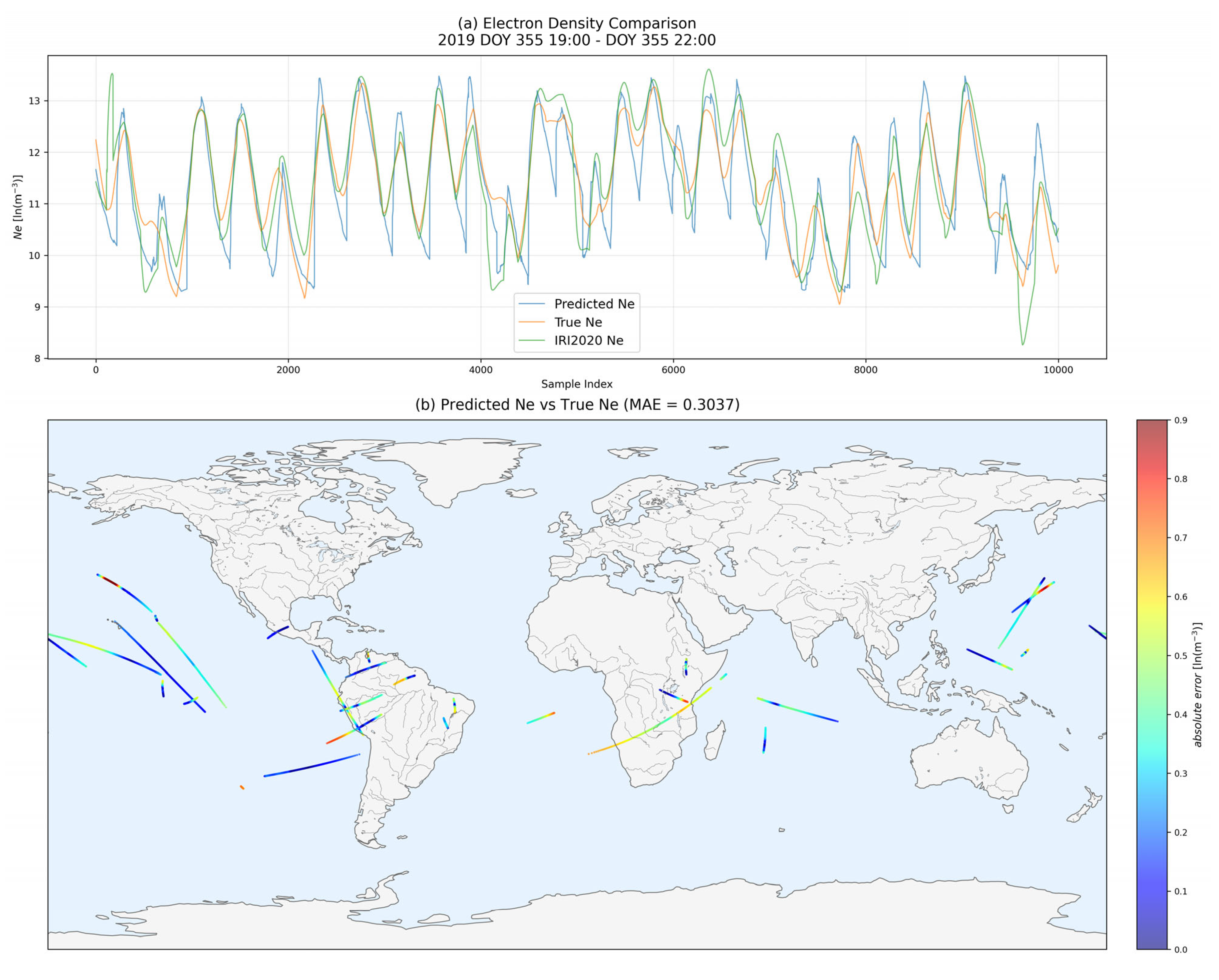
3.2. Comparison with COSMIC-2 Satellite Observations

To validate the model’s generalization capability, preprocessed COSMIC-2 radio occultation data—including spatiotemporal coordinates (longitude, latitude, altitude, UTC time)—along with contemporaneous TEC, AE, SYM-H, and F10.7 parameters were fed into the decomposition model to obtain predicted electron densities. For comparative analysis, IRI-2020 outputs were generated under identical input conditions, with COSMIC-2 observations serving as the benchmark for dual-model performance evaluation.

Due to significant measurement noise from observational instruments, a moving average filter with a window size of 180 was applied to all three Ne datasets (predicted/IRI-2020/observed), effectively suppressing small-scale ionospheric irregularities and mitigating outlier impacts. Figure 6 displays comparative results during a representative time window (19:00–22:00 UTC on 2019 DOY 355).

The metrics applied in this section are defined as follows:

$$absolute error=\left|\mathrm{y}-\widehat{y}\right|$$

(4)

$$MAE={\displaystyle \frac{1}{n}}\sum _{i=1}^n\left|y_i-\widehat{y_i}\right|$$

(5)

$$MSE={\displaystyle \frac{1}{n}}\sum _{i=1}^n{\left(y_i-\widehat{y_i}\right)}^2$$

(6)

In these equations,

• Equation (4) represents the absolute error for individual data points.
• Equations (5) and (6) correspond to the mean absolute error (MAE) and mean squared error (MSE), respectively.
• $y_i$: Predicted values from either the decomposition model or IRI-2020.
• $\widehat{y_i}$: Observed values from COSMIC-2.

Detailed metric values are provided in

Table 2. Metrics of Ne among COSMIC-2, decomposition model, and IRI-2020.

Statistics and Metrics	COSMIC-2	Decomposition Model	IRI-2020
Mean	11.3987	11.2849	11.4355
Std	0.9806	1.1236	1.1418
Max	13.3330	13.4746	13.6078
Min	9.0494	9.2830	8.2590
MSE	-	0.1389	0.3202
RMSE	-	0.3726	0.5659
MAE	-	0.3037	0.4269
Std of Abs Error	-	0.2159	0.3714
R2	-	0.8574	0.6675

.

Long-term statistical metrics for 2019 (encompassing all COSMIC-2 observational data from that year) are presented in Figure 7. Each point along the satellite orbital trajectory represents an individual observation event, with color coding reflecting the magnitude of the absolute error values.

4. Discussion

This study pioneers the first successful implementation of a deep learning-based Multilayer Perceptron (MLP) framework to achieve global-scale mapping from macroscale IGS-TEC data to the vertically layered electron density (Ne), while integrating geomagnetic (AE, SYM-H) and solar activity (F10.7) parameters. This novel framework demonstrates the transformative potential of data-driven methodologies in advancing ionospheric modeling. The discussion proceeds across three dimensions: model performance, application value, and inherent limitations.

(1)

Model Performance

The experimental results demonstrate that the electron density derived from TEC decomposition achieves significant accuracy improvements over the conventional IRI-2020 model, alongside remarkably faster inference speeds. The model effectively exploits readily observable TEC data to decompose them into vertically layered Ne profiles with enhanced precision. Beyond accuracy, the model demonstrates a significant advantage in computational efficiency during inference. For example, in a test case using 10,000 data points, our deep learning model completed the inference in a few seconds, whereas the IRI-2020 model required several minutes to process the same number of points. This substantially faster inference speed makes the decomposition model highly suitable for applications requiring near real-time or real-time electron density information.

(2)

Application Value and Limitations

The proposed framework demonstrates significant accuracy improvements over conventional IRI-2020 in electron density reconstruction, while achieving sub-second inference speeds. This success aligns with neural-network approaches for ionospheric tomography, particularly the Residual Minimization Training Neural Network (RMTNN) methodology that has proven effective in resolving ill-posed problems under sparse observational constraints [28]. Unlike previous regional-scale RMTNN implementations constrained by ground-based GPS receivers [28,29], our model innovates through two aspects: (a) global-scale generalization enabled by assimilating macroscale TEC patterns rather than localized slant TEC measurements; (b) explicit incorporation of space weather drivers (AE/SYM-H/F10.7) to capture storm-time ionospheric dynamics. The vertical resolution (~30 km) matches state-of-the-art neural tomography techniques [29] while overcoming their dependence on ionosonde-assisted altitude corrections through end-to-end TEC decomposition learning.

However, the model exhibits two key limitations:

• A common limitation of purely data-driven AI models in geophysical applications, including the present study, is their limited physical interpretability. The absence of explicit ionospheric dynamical equations (e.g., continuity and momentum equations) in such frameworks restricts direct insight into underlying physical processes.
• Extreme Space Weather Generalization: This study does not focus on the generalization performance of extreme space weather periods, which is worthy of further verification in the following.

Future research can optimize the model performance from three aspects: (a) Integrating physics-informed approaches, such as Physics-Informed Neural Networks (PINNs) or incorporating physics-based regularization terms in the loss function (e.g., enforcing electron density vertical gradient conservation or adherence to aspects of ionospheric dynamical equations), to balance data-driven flexibility with physical consistency. This direction follows paradigms like the RMTNN approach of objective function minimization [29] but explicitly leverages physical principles. (b) Adopting graph neural networks (GNNs) or Transformer architectures to explicitly model global spatiotemporal correlations of ionospheric parameters [30]. (c) Incorporating real-time Ne observations from low-Earth orbit (LEO) satellites (e.g., Swarm) to enhance generalization via multi-source data assimilation. Furthermore, extending the model to ionospheric disturbance propagation tracking would amplify its operational utility in space weather services.

5. Conclusions

This study establishes the first deep learning-based Ionospheric Vertical Decomposition Framework (IVDF) that combines global coverage (by leveraging globally assimilated TEC), integrated space weather indices (AE/SYM-H/F10.7), and capabilities supporting real-time applicability for the high-precision mapping of macroscale TEC to vertically layered electron density (Ne) profiles spanning 60–800 km. The marked performance improvements validate the potential of data-driven approaches fused with space physics parameters, while also revealing the need to deepen “data-physics” synergistic modeling mechanisms under complex space weather events. This work not only advances a novel technical pathway for ionospheric research but also lays critical foundations for near-space environment monitoring and geomagnetic hazard warning systems.

References

1. Jakowski, N.; Mayer, C.; Hoque, M.M.; Wilken, V. Total Electron Content Models and Their Use in Ionosphere Monitoring. Radio Sci. 2011, 46, RS0D18. [Google Scholar] [CrossRef]
2. Köhnlein, W. Electron Density Models of the Ionosphere. Rev. Geophys. 1978, 16, 341–354. [Google Scholar] [CrossRef]
3. Peng, J.; Yuan, Y.; Liu, Y.; Zhang, H.; Zhang, T.; Wang, Y.; Dai, Z. Evaluation of GNSS-TEC Data-Driven IRI-2016 Model for Electron Density. Atmosphere 2024, 15, 958. [Google Scholar] [CrossRef]
4. Patel, K.; Chaurasiya, S.K. Geomagnetic Storms and Their Effect on Global Positioning System: A Supplication of Global Navigation Satellite System Receivers. In GNSS Applications in Earth and Space Observations; CRC Press: Boca Raton, FL, USA, 2025; pp. 265–279. [Google Scholar]
5. Bothmer, V.; Daglis, I.A.; Arbesser-Rastburg, B.; Jakowski, N. Effects on Satellite Navigation. In Space Weather—Physics and Effects; Bothmer, V., Daglis, I.A., Eds.; Springer: Berlin/Heidelberg, Germany, 2007; pp. 383–402. [Google Scholar]
6. Huang, X.; Reinisch, B.W. Vertical Electron Density Profiles from the Digisonde Network. Adv. Space Res. 1996, 18, 121–129. [Google Scholar] [CrossRef]
7. Nava, B.; Radicella, S.M.; Leitinger, R.; Coïsson, P. Use of Total Electron Content Data to Analyze Ionosphere Electron Density Gradients. Adv. Space Res. 2007, 39, 1292–1297. [Google Scholar] [CrossRef]
8. Mengist, C.K.; Yadav, S.; Kotulak, K.; Bahar, A.; Zhang, S.R.; Seo, K.H. Validation of International Reference Ionosphere Model (IRI-2016) for F-Region Peak Electron Density Height (hmF2): Comparison with Incoherent Scatter Radar (ISR) and Ionosonde Measurements at Millstone Hill. Adv. Space Res. 2020, 65, 2773–2781. [Google Scholar] [CrossRef]
9. Reinisch, B. Ionosphere and Plasmasphere Electron Density Profiles. In Proceedings of the 2014 XXXIth URSI General Assembly and Scientific Symposium (URSI GASS), Beijing, China, 16–23 August 2014; pp. 1–2. [Google Scholar]
10. Ma, Q.; Xu, W.; Sanchez, E.R.; Marshall, R.A.; Bortnik, J.; Reyes, P.M.; Tam, S.Y. Analysis of Electron Precipitation and Ionospheric Density Enhancements Due to Hiss Using Incoherent Scatter Radar and Arase Observations. J. Geophys. Res. Space Phys. 2022, 127, e2022JA030545. [Google Scholar] [CrossRef]
11. Liu, J.Y.; Lin, C.H.; Rajesh, P.K.; Lin, C.Y.; Chang, F.Y.; Lee, I.T.; Chen, S.P. Advances in Ionospheric Space Weather by Using FORMOSAT-7/COSMIC-2 GNSS Radio Occultations. Atmosphere 2022, 13, 858. [Google Scholar] [CrossRef]
12. Jiang, C.; An, Q.; Wang, S.; Nie, W.; Zhu, H.; Liu, G. Accuracy Assessment of the Ionospheric Total Electron Content Derived from COSMIC-2 Radio Occultation Based on Multi-Source Data. Adv. Space Res. 2024, 73, 5157–5170. [Google Scholar] [CrossRef]
13. World Meteorological Organization. COSMIC-2. WMO OSCAR—Details for Instrument TGRS (COSMIC-2). Available online: https://space.oscar.wmo.int/satellites/view/cosmic_2 (accessed on 6 May 2025).
14. Seemala, G.K. Estimation of Ionospheric Total Electron Content (TEC) from GNSS Observations. In Atmospheric Remote Sensing; Elsevier: Amsterdam, The Netherlands, 2023; pp. 63–84. [Google Scholar]
15. Jakowski, N.; Hoque, M.M. Estimation of Spatial Gradients and Temporal Variations of the Total Electron Content Using Ground-Based GNSS Measurements. Space Weather 2019, 17, 339–356. [Google Scholar] [CrossRef]
16. She, C.; Yue, X.; Hu, L.; Zhang, F. Estimation of Ionospheric Total Electron Content from a Multi-GNSS Station in China. IEEE Trans. Geosci. Remote Sens. 2019, 58, 852–860. [Google Scholar] [CrossRef]
17. Chen, Z.; Liao, W.; Li, H.; Wang, J.; Deng, X.; Hong, S. Prediction of Global Ionosphere TEC Based on Deep Learning. Space Weather 2022, 20, e2021SW002854. [Google Scholar] [CrossRef]
18. Liu, L.; Zou, S.; Yao, Y.; Wang, Z. Forecasting Global Ionospheric TEC Using Deep Learning Approach. Space Weather 2020, 18, e2020SW002501. [Google Scholar] [CrossRef]
19. Wen, Z.; Li, S.; Li, L.; Wu, B.; Fu, J. Ionospheric TEC Prediction Using Long Short-Term Memory Deep Learning Network. Astrophys. Space Sci. 2021, 366, 3. [Google Scholar] [CrossRef]
20. Ruwali, A.; Kumar, A.S.; Prakash, K.B.; Sivavaraprasad, G.; Ratnam, D.V. Implementation of Hybrid Deep Learning Model (LSTM-CNN) for Ionospheric TEC Forecasting Using GPS Data. IEEE Geosci. Remote Sens. Lett. 2020, 18, 1004–1008. [Google Scholar] [CrossRef]
21. Nayak, K.; Romero-Andrade, R.; Sharma, G.; López-Urías, C.; Trejo-Soto, M.E.; Vidal-Vega, A.I. Evaluating Ionospheric Total Electron Content (TEC) Variations as Precursors to Seismic Activity: Insights from the 2024 Noto Peninsula and Nichinan Earthquakes of Japan. Atmosphere 2024, 15, 1492. [Google Scholar] [CrossRef]
22. Nayak, K.; Romero-Andrade, R.; Sharma, G.; Zavala, J.L.C.; Urias, C.L.; Trejo-Soto, M.E.; Aggarwal, S.P. A combined approach using b-value and ionospheric GPS-TEC for large earthquake precursor detection: A case study for the Colima earthquake of 7.7 Mw, Mexico. Acta Geodaet. Geophys. 2023, 58, 515–538. [Google Scholar] [CrossRef]
23. Gao, S.; Cai, H.; Zhan, W.; Wan, X.; Xiong, C.; Zhang, H.; Xu, C. Characterization of Local Time Dependence of Equatorial Spread F Responses to Substorms in the American Sector. J. Space Weather Space Clim. 2023, 13, 2. [Google Scholar] [CrossRef]
24. Swarnalingam, N.; Wu, D.L.; Gopalswamy, N. Interhemispheric Asymmetries in Ionospheric Electron Density Responses During Geomagnetic Storms: A Study Using Space-Based and Ground-Based GNSS and AMPERE Observations. J. Geophys. Res. Space Phys. 2022, 127, e2021JA030247. [Google Scholar] [CrossRef]
25. Liou, Y.A.; Pavelyev, A.G.; Liu, S.F.; Pavelyev, A.A.; Yen, N.; Huang, C.Y.; Fong, C.J. FORMOSAT-3/COSMIC GPS Radio Occultation Mission: Preliminary Results. IEEE Trans. Geosci. Remote Sens. 2007, 45, 3813–3826. [Google Scholar] [CrossRef]
26. Schreiner, W.S.; Weiss, J.P.; Anthes, R.A.; Braun, J.; Chu, V.; Fong, J.; Zeng, Z. COSMIC-2 Radio Occultation Constellation: First Results. Geophys. Res. Lett. 2020, 47, e2019GL086841. [Google Scholar] [CrossRef]
27. Bilitza, D.; Pezzopane, M.; Truhlik, V.; Altadill, D.; Reinisch, B.W.; Pignalberi, A. The International Reference Ionosphere Model: A Review and Description of an Ionospheric Benchmark. Rev. Geophys. 2022, 60, e2022RG000792. [Google Scholar] [CrossRef]
28. Hirooka, S.; Hattori, K.; Takeda, T. Numerical Validations of Neural-Network-Based Ionospheric Tomography for Disturbed Ionospheric Conditions and Sparse Data. Radio Sci. 2011, 46, RS5011. [Google Scholar] [CrossRef]
29. Ma, X.F.; Maruyama, T.; Ma, G.; Takeda, T. Three-Dimensional Ionospheric Tomography Using Observation Data of GPS Ground Receivers and Ionosonde by Neural Network. J. Geophys. Res. 2005, 110, A05308. [Google Scholar] [CrossRef]
30. Liu, R.; Jiang, Y. Ionospheric VTEC Maps Forecasting Based on Graph Neural Network With Transformers. IEEE J. Sel. Top. Appl. Earth Obs. Remote Sens. 2025, 18, 1802–1816. [Google Scholar] [CrossRef]
Figure 1. Heatmap of the global TEC value distribution. The figure shows the global TEC distribution at 12:00 UTC on 21 March 2011. A pronounced peak appears near the equatorial region and subsolar point, consistent with solar irradiance-driven ionization enhancement. TEC is expressed in TEC units (TECU), where 1 TECU = 1016 electrons/m2. The observed values range from approximately 5 to over 60 TECU, reflecting significant regional and latitudinal variation. This global distribution highlights the macroscale structure of the ionosphere and forms the input basis for the vertical electron density reconstruction discussed in later sections.
Atmosphere 16 00598 g001
Figure 2. Three-dimensional multilayer heatmap of electron density. The figure shows the layered distribution of the global electron density by altitude at 12:00 UTC on March 21, 2011. Electron density is expressed in natural logarithmic scale (ln(m−3)) to accommodate its wide dynamic range. The plot reveals altitude-dependent features of the ionosphere, including dense equatorial ionization near 300 km (F-layer) and weaker ionization at higher and lower altitudes.
Atmosphere 16 00598 g002
Figure 3. Histogram and kernel density estimation (KDE) of COSMIC-2 satellite-derived electron density profile altitudes for the period DOY 274–365 in 2019. The histogram illustrates the frequency distribution of valid altitude samples after data cleaning, ranging from 60.0 km to 727.55 km. A KDE curve (red) is overlaid to reveal the continuous density trend, with the mean altitude marked at 416.9 km (σ = 171.10). The distribution reflects COSMIC-2’s high coverage in the F-region ionosphere, supporting its suitability as a benchmark dataset for evaluating the model-reconstructed electron density profiles.
Atmosphere 16 00598 g003
Figure 4. Model input–output workflow diagram. Schematic diagram illustrating the workflow of the Multilayer Perceptron (MLP) model used for ionospheric vertical decomposition. Inputs to the model include the following: (1) Spatiotemporal data (e.g., geographic coordinates, time). (2) 2D Total Electron Content (TEC) maps derived from IGS data, representing the macroscale ionospheric state. (3) Space environment parameters, specifically geomagnetic indices (AE, SYM-H) and the solar activity index (F10.7), capturing external driving factors. The MLP processes these combined features to predict the primary output: a vertically layered electron density (Ne) profile covering the 60–800 km altitude range.
Atmosphere 16 00598 g004
Figure 5. Model performance on the 2019 test set. (a) Vertical profiles of R2 (coefficient of determination, red) and RMSE (root mean square error, yellow) scores, evaluating the agreement between the predicted and ground truth ln(Ne) as a function of altitude (60–800 km). Ionospheric regions (D, E, F) are indicated. (b) Comparison of global ln(Ne) maps (units: ln(m−3)). Side-by-side plots compare the ground truth (“Reconstructed”) electron density patterns with the model’s predictions (“Predicted”) at selected altitudes (300, 500, 700 km) and specific times (2019-03-21 12:00 UT and 2019-09-23 20:00 UT).
Atmosphere 16 00598 g005
Figure 6. (a) A line graph showing the comparison between the predicted electron density by the decomposition model, the predicted electron density by IRI-2020 and the observed data from 19:00 to 22:00 on the 355th day of 2019. Lines represent Nepred (blue), Neobs (orange), and NeIRI (green). (b) Satellite orbit display of the same time period, with colors corresponding to the magnitude of the absolute error. The corresponding mean absolute error (MAE = 0.3037 ln(m−3)) is shown.
Atmosphere 16 00598 g006
Figure 7. Global distribution and orbital coverage of COSMIC-2 observational data points from day of the year (DOY) 274 to 365 in 2019. Each point represents an individual observation event along the satellite trajectory, with its color indicating the magnitude of the absolute error in units of ln(m−3). The corresponding mean absolute error (MAE = 0.598387 ln(m−3)) is shown.
Atmosphere 16 00598 g007