Improving Weather Forecasting in Remote Regions Through Machine Learning

Abstract

The accuracy of weather forecasting hinges crucially on the availability of comprehensive historical weather data. In remote regions face the challenge of sparse data collection, impacting the accuracy of meteorological predictions. This study delves into the data scarcity issue and its repercussions on weather forecasting in these regions. By evaluating the Meteorological Data Supply Portal of the India Meteorological Department and various climatic classifications, this paper gain insights into the present state of weather data accessibility and identify the regions with substantial gaps. This study investigates the extent to which Machine Learning Techniques can compensate for these deficiencies. By leveraging advanced machine learning and deep learning techniques on available data from well-documented regions, this paper propose a framework for generating reliable weather forecasts for remote territories. This paper not only highlights the current landscape of meteorological data availability in remote areas but also examines the potential of ML to democratize weather forecasting, thereby enabling better-preparedness for adverse weather conditions in these underserved regions. The hypothesis of this paper contends that with sufficient training on diverse datasets, ML can provide a significant predictive advantage, serving as a testament to the ingenuity of modern computational methods in confronting real-world challenges. Here, the deep learning model achieves a notable accuracy of 83%, showcasing a substantial improvement over traditional rule-based system. The integration of ML not only enhanced predictive accuracy but also demonstrated a nuanced understanding of complex weather dynamics through data-driven insights.

1. Introduction

Artificial Intelligence (AI) has progressively become an integral component of various fields, revolutionizing processes and outcomes through its advanced computational capabilities. In the realm of meteorology, AI and machine learning algorithms have demonstrated significant potential to enhance the accuracy of weather forecasts. These technologies process large volumes of data, identify complex patterns, and provide insights that were previously unattainable through traditional methods. The advent of AI in weather prediction has opened avenues for advancements in disaster management, agriculture, and several other sectors that rely heavily on accurate weather information. Despite these technological advancements, traditional weather forecasting methods continue to struggle, particularly in regions where historical weather data is not abundantly available. Remote and lessdocumented areas often lack the necessary infrastructure to collect and archive weather information, leading to substantial gaps in the data necessary for accurate forecasting. This deficiency impacts not only the predictability of weather phenomena but also poses risks to local communities that depend on accurate weather information for agriculture, disaster preparedness, and daily activities. The primary goal of this research is to harness the power of AI to mitigate the challenges posed by sparse data in traditional weather forecasting methods. By leveraging advanced algorithms and data processing techniques, this study aims to improve the predictability of weather phenomena in data-deficient areas. The intent is to explore innovative ways in which AI can be utilized to interpret limited data, enhance data extrapolation, and offer reliable weather forecasts for regions where historical data is not comprehensive. This investigation hypothesizes that AI can effectively use comprehensive datasets from well-documented cities to predict weather in lesser-documented regions, thus filling the void left by the unavailability of historical data. By training AI models with extensive data from various locations, these models could learn to identify broader weather patterns and apply this knowledge to generate forecasts for areas with similar climatic conditions but insufficient historical data. The research will assess the feasibility of this approach and its potential to improve forecast accuracy in remote parts, which are currently underserved in terms of weather prediction capabilities.

2. Literature Review

The journey of artificial intelligence in weather forecasting began with rule-based systems, where predictions were made based on a predefined set of rules derived from historical weather patterns. The early systems might have used linear regression models to predict rainfall based solely on variables like temperature or humidity. However, such models often failed to capture the intricate relationships between multiple factors influencing rainfall patterns, leading to limited accuracy in predictions.

2.1. Weather Prediction Using Numerical Weather Prediction (NWP) Methods

The basic numerical weather prediction is forecasted by integrating the NWP with prediction equations for better understanding the system [1], and its current state and challenges [2]. Authors concentrated only on data driven predictions of the medium range global atmospheric flow [3]. In daily use and history of NWP from 1954 to 1989 is discussed [4,5]. In paper [6] the fundamentals of numerical approaches for weather forecasting issues are covered. The relevance of numerical weather prediction for forecasting natural hazards, for monitoring the global environment, and importance in energy forecast is discussed [7,8]. In paper [9] advancements are made possible by the physical parameterization techniques, introducing new or enhanced forms of observation, improving the data-assimilating processes, and improving the models’ vertical and horizontal resolutions. Tables have been deleted as suggested.

2.2. Weather Prediction Using Machine Learning Techniques

The integration of machine learning (ML) with weather forecasting marked a significant leap forward. Unlike rule-based systems, ML algorithms learn from data, identifying patterns and making predictions based on historical trends. For instance, ML models could analyze a combination of variables such as temperature, humidity, wind speed, and atmospheric pressure to forecast rainfall probabilities with better accuracy. This shift allows for more dynamic models [10] that could adapt new information, significantly improving the accuracy of weather forecasts. It is analyzed that 500 most pertinent scientific articles are published during 2018 that addresses machine learning techniques in the field of climate and numerical weather prediction [11]. The Support Vector Machine (SVM), Artificial Neural Network (ANN), and Time Series Recurrent Neural Network (RNN) machine learning models for weather prediction are examined [12]. In paper [13] various machine learning techniques discussed for weather prediction.The degree to which different word overlap measures connect to the human-rated similarity of reference and forecasted summaries are measured through experimentation [14]. The study presented various machine learning algorithms that were trained on historical data and then used to forecast weather with an accuracy that surpasses the traditional techniques [15]. The authors suggested a model for weather prediction based on neural networks. The Indian Metrological Department’s (IMD) meteorological data is used to test the suggested model’s superiority [16]. To predict variables like air temperature (T) and relative humidity (Rh), several machines learning algorithms, including gradient boosting tree (G.B.T.), random forest (R.F.), linear regression (LR), and various artificial neural network (ANN) architectures multi-layered perceptron and radial basis function are suggested [17]. Paper [18] proposed a machine learning-based weather forecasting model. Four classifier algorithms the Random Forest, the Decision Tree, the Gaussian Naïve Bayes and the Gradient Boosting are used to implement the model. The algorithms are trained on a publicly accessible dataset from Kaggle that covered the city of Seattle from 2012 to 2015. The five machine-learning algorithms to predict meteorological parameters, including temperature, wind direction, speed, pressure, humidity, and cloudiness. Tests are conducted at four different locations in Mauritius [19]. Based on performance measures, including confusion matrix measurements, algorithms including Gradient Boosting, AdaBoosting, Artificial Neural Network, Stacking Random Forest, Stacking Neural Network, and Stacking k-nearest neighbors (KNN) are assessed and contrasted [20].

2.3. Weather Prediction Using Deep Learning Techniques

Deep learning (DL), a subset of machine learning characterized by algorithms known as neural networks, has further revolutionized weather forecasting. With its advanced pattern recognition capabilities, deep learning [21,22] can analyze vast datasets [10], including satellite imagery and atmospheric data, to identify patterns that elude traditional models. For example, convolutional neural networks (CNNs) can analyze satellite images to detect cloud formations associated with rainfall, enabling more accurate predictions of precipitation events [23]. In order to forecast weather given historical data from two locations in London, this study looks at deep learning [24]. In this study, hourly forecasts of the 2 m temperature for the next 12 h over Europe are created using an advanced generative network called the Stochastic Adversarial Video Prediction (SAVP) model and a basic recurrent neural network with convolutional filters called ConvLSTM [25]. The authors addressed the possibility of fully substituting DL techniques for the existing numerical weather models and data assimilation systems [26]. The authors provide an overview of the most recent research on deep learning-based weather forecasting, covering topics such as neural network (NN) architectural design, temporal and geographical scales, datasets, and benchmarks [27]. Researchers demonstrated a neural network that can accurately forecast precipitation up to 12 h in advance. The model beats state-of-theart physics-based models currently in use in the Continental United States, with up to 12 h of lead time, in terms of raw precipitation targets projected [28]. Enhancing data from a small number of input atmospheric condition variables, a data-driven model trained to predict intricate surface temperature patterns. The model generates a genuine seasonal cycle on annual time scales that is exclusively fueled by the specified variance in solar forcing at the top of the atmosphere [29] and explore weather forecasting using deep learning approaches. The prediction performance of the Recurrence Neural Network (RNN), Conditional Restricted Boltzmann Machine (CRBM), and Convolutional Network (CN) models specifically compared [30]. In order to accurately anticipate air temperature over two forecast horizons, this work investigates the application of deep learning models to air temperature forecasting [31]. The authors described creating and assessing a unique and lightweight weather forecasting system with contemporary neural networks [32]. The authors suggested a hybrid model that combines deep neural network post-processing with a small portion of the original meteorological trajectories. These allow the model to take into account non-linear correlations that are not taken into account by the numerical models or post-processing techniques used at the moment [33].

2.4. Weather Prediction Using Large Language Models (LLMs)

Large Language Models (LLMs) [34] have transformed how meteorologists and researchers interpret and communicate weather data. These models, trained on diverse datasets, can understand and generate natural language, making it easier to communicate complex weather forecasts to the public and decision-makers. For instance, LLMs can analyze textual weather reports and extract key information about rainfall predictions, providing succinct summaries that are easily understandable by non-experts. This study investigates whether machine learning techniques can offer a different method for determining how much future weather forecasts might differ from the baseline [35]. The authors suggested LLM4TS, a framework for time-series forecasting [36] with pre-trained LLMs. This article focuses on Time-series alignment, which matches LLMs with the nuances of time-series data, and forecasting fine-tuning, which is utilized for jobs involving time-series forecasting downstream, are the two phases of LLM4TS’s finetuning technique [37]. In this paper, authors argued that the latest LLMs have the potential to revolutionize time series analysis, enabling efficient decision-making and advancing the field towards a more comprehensive kind of time series analytical intelligence [38]. The authors introduced TIME-LLM, a reprogramming framework that allows LLMs to be used for generic time series forecasting while maintaining the structural integrity of the language models. The authors first reprogrammed the input time series using text prototypes before feeding it into the frozen LLM then align the two modalities [39].

2.5. Weather Prediction Using Generative AI

Generative AI [40] represents the frontier in leveraging AI for weather forecasting, with the potential to generate novel content and actionable insights from large datasets. By simulating different weather scenarios based on existing data, generative AI [41] models can help forecasters prepare for a wide range of outcomes, including extreme weather events. For example, generative adversarial networks (GANs) can generate synthetic weather data based on historical records, allowing researchers to explore hypothetical scenarios and assess their potential impact on rainfall patterns. In this paper the authors predicted, the geopotential height of the 500 hPa pressure level, the two-meter temperature, and the overall amount of precipitation over the course of the following 24 h over Europe, using a conditional deep convolutional generative adversarial network [42]. The authors suggested using deep generative diffusion models trained on historical data to simulate these forecasts and so amortise the computational cost. The trained models may sample hundreds of actual weather forecasts at minimal cost, and they are extremely scalable with respect to high-performance computer accelerators [43]. In this paper the authors offered a ground-breaking Transformer-based weather forecasting model. The proposed Tensorial Encoder Transformer (TENT) model can analyse meteorological data in multidimensional tensorial format, enabling it to use the spatiotemporal structure of the data, since it possesses tensorial attention [44]. The authors proposed methodology that shown exceptional dependability and efficacy, furnishing valuable insights to diverse industries and sectors, including emergency response planning, transportation, and agriculture, which are reliant on accurate meteorological data. The merging of transformer models with the Internet of Things signal has resulted in significant advancements in weather and climate modelling [45]. In this paper for post-processing numerical weather prediction (NWP) forecasts of 2 m air temperature, a novel technique based on the Transformer model is put forth [46]. The authors proposed a new method based on the Transformer model for post-processing 2 m air temperature numerical weather prediction (NWP) forecasts [47].

3. Methodology

Our methodology initially identifies a well-documented region and then authors applied machine learning algorithms to solve the data scarcity issue on a remote region by extracting the features for effective prediction (see Figure 1).

3.1. Data Collection

In this paper, the data collection efforts were meticulously organized to encompass a wide array of weather parameters alongside vital city characteristics, emphasizing cities across India. In pursuit of a holistic understanding of the factors influencing weather phenomena, we leveraged multiple reliable sources to compile datasets that extend beyond conventional weather metrics. A significant portion of our weather data was sourced from the Historical Hourly Weather Data available on Kaggle, which provided us with an extensive array of basic weather metrics across various global cities, including temperature, humidity, pressure, wind direction, and wind speed. This dataset can be accessed at [48] https://www.kaggle.com/datasets/selfishgene/historical-hourly-weather-data/data (accessed on 10 Ocober 2024), offering valuable insights into historical weather patterns over several years. Utilizing this dataset as a foundational component, we further enriched our analysis with additional city-specific characteristics to deepen our understanding of local climatic influences. In addition to the standard atmospheric conditions, our data collection process distinguished itself by integrating city-specific characteristics. These include geographical positioning, proximity to significant water bodies, elevation levels, and more. Such an approach ensures that our analysis respects the intricate interplay between local environmental features and weather patterns. Our concerted efforts culminated in the creation of a generic dataset, meticulously assembled by enriching the standard weather data from Kaggle with city attributes, providing a multidimensional perspective on weather forecasting. This dataset spans over 1.2 million entries, with observations from 27 cities worldwide, including several from India. It encompasses 23 distinct columns, covering a diverse range of data types from floating-point numbers to categorical strings, underlining the dataset’s complexity and richness.

Key Components of This Dataset Includes

• Basic Weather Metrics: Temperature, humidity, pressure, wind direction, and wind speed, serving as the foundation of our weather forecasting model.
• Rain Indicator: A binary variable indicating the presence of rain, derived from detailed weather descriptions, to facilitate precise precipitation forecasting.
• Geographical and Environmental Features: Data on cities’ latitude, longitude, elevation, and their proximity to rivers, lakes, oceans, and deserts. These factors are crucial for understanding the local climate’s unique characteristics.
• City Attributes: Information on land cover, prevailing winds, and ocean currents, providing insights into the environmental and climatic influences on weather patterns.
• Socio-Environmental Indicators: Nearness to rivers, lakes, oceans, and deserts, alongside detailed descriptors of water body sizes and environmental settings, offering a nuanced view of each city’s susceptibility to various weather phenomena.

In this paper, we meticulously gathered datasets encompassing various weather parameters and city characteristics from multiple reliable sources, focusing particularly on cities across India [49]. In addition to conventional weather variables like temperature, humidity, pressure, wind direction, and wind speed, we included several additional features specific to the Indian context:

• Average Annual Temperature (°C): Providing insights into the typical temperature patterns experienced by each city throughout the year, influencing local climate dynamics and seasonal variations.
• Average Annual Rainfall (mm): Describing the amount of precipitation received by each city annually, a crucial factor in understanding its susceptibility to droughts, floods, and other weather-related phenomena.
• Humidity Levels (%): Reflecting the moisture content in the air, humidity levels play a vital role in determining the comfort level, as well as influencing precipitation and atmospheric stability.
• Population Density (people/km²): Highlighting the concentration of inhabitants within each city’s geographical area, population density serves as a proxy for urbanization, resource demand, and infrastructure resilience.
• Industrial Activity: Assessing the extent of industrialization and manufacturing activities within city limits, which can contribute to air pollution, heat island effects, and local microclimates.
• Average Air Quality Index (AQI): Quantifying the overall air quality based on pollutant levels, the AQI serves as a critical indicator of environmental health and public well-being, influencing respiratory health and weather patterns.
• Historical Weather Extremes: Documenting past instances of extreme weather events, including heatwaves, cyclones, and heavy rainfall, to gauge each city’s vulnerability and resilience to climate-related hazards.
• Solar Radiation (kWh/m²/day): Estimating the solar energy potential available in each city, solar radiation data informs renewable energy planning and sustainable development initiatives.
• Nearness to River/Lake/Ocean: Indicating the proximity of each city to significant water bodies, which can influence local weather patterns, especially during monsoon seasons.
• Size of River/Lake/Ocean: Providing information on the scale of nearby water bodies, which may affect humidity levels and precipitation rates.
• Nearness to Desert: Highlighting cities located near arid regions, which experience distinct weather phenomena and temperature extremes.
• Elevation in Meters: Reflecting the altitude of each city above sea level, which can impact temperature variations and atmospheric pressure.
• Land Cover and Vegetation: Describing the dominant land cover types in and around each city, influencing local microclimates and heat absorption.
• Prevailing Winds and Ocean Currents: Identifying prevailing wind directions and ocean currents that influence weather patterns, particularly along coastal regions.

These additional features are crucial for capturing the unique climatic characteristics of Indian cities and enhancing the accuracy of our predictive models.

3.2. Incorporating New Features for Enhanced Predictions

Incorporating specific features into the dataset, particularly for a diverse and climatically complex country like India, significantly enhances the predictive accuracy and relevance of AI-driven weather forecasting models. Each of these features brings a unique dimension to understanding and predicting weather patterns, taking into account not only meteorological factors but also geographical, environmental, and human factors that influence weather outcomes. Here’s how adding these features specifically benefits the forecasting model in the context of India.

• Average Annual Temperature (°C)

India’s vast geographic spread encompasses a wide range of climatic zones, from the cold Himalayan north to the tropical south. By including the average annual temperature, the model can better adapt its predictions to the inherent climatic variations across different regions, providing insights into the broader climate dynamics and seasonal variations that impact weather patterns significantly. The Clausius-Clapeyron equation gives a basic estimation of the saturation vapor pressures es as a function of temperature, which can be used to approximate the potential for precipitation:

$$e_s\left(T\right)=e_0.exp\left[{\displaystyle \frac{L_v}{R_v}}({\displaystyle \frac{1}{T_0}}-{\displaystyle \frac{1}{T}})\right]$$

(1)

where: $e_0$ is the saturation vapor pressure at a reference temperature $T_0$, $L_v$ is the latent heat of vaporization, $R_v$ is the specific gas constant for water vapor, and T is the temperature in Kelvin.

• Average Annual Rainfall (mm)

Rainfall in India is highly variable and critically influences agriculture, water resources, and disaster management practices. The monsoon season, in particular, has a profound impact on the country’s agricultural output and water supply. Incorporating average annual rainfall data helps the model predict potential droughts or floods, enabling more effective water resource management and agricultural planning.

• Humidity Levels (%)

Humidity affects comfort levels, precipitation patterns, and the formation of weather phenomena such as fog and dew. Given India’s tropical and subtropical climates, humidity plays a crucial role in daily weather patterns, especially in coastal regions. By analyzing humidity levels, the model can offer more accurate forecasts regarding precipitation and atmospheric stability.

• Population Density (people/km²)

Population density is a crucial factor in urban microclimate dynamics. High-density areas, especially large cities, tend to experience heat island effects, wherein urban regions are significantly warmer than their rural counterparts. This feature allows the model to consider the impact of urbanization on temperature and weather patterns, enhancing the forecasts’ relevance to densely populated areas. The heat island intensity (IHI) can be related to population density ($\rho$) through an empirical relationship:

$$I_{HI}=K.log\left(\rho \right)$$

(2)

K is a constant that varies depending on local conditions and urban geometry, $\rho$ is the population density. This equation underscores the impact of urbanization (as indicated by population density) on local temperature elevations, which are crucial for accurate weather forecasting in urban areas.

• Industrial Activity

The level of industrial activity affects local air quality and can contribute to the formation of heat islands. In India, where industrial hubs are often located near or within densely populated areas, the impact on local weather patterns, including temperature and air quality, is significant. Incorporating this feature helps in understanding and predicting the microclimatic effects of industrialization. The impact of industrial activity on air quality, particularly the concentration of a pollutant (C), can be simplified as:

$$C={\displaystyle \frac{Q}{u.H.W}}$$

(3)

where: Q is the pollutant emission rate from industrial sources, u is the wind speed, H and W are the height and width of the emission plume dispersion area. This formula highlights how industrial emissions, modulated by local wind patterns, contribute to variations in air quality, influencing weather phenomena like fog formation and precipitation acidity.

• Average Air Quality Index (AQI)

Air quality directly influences respiratory health and can affect weather patterns, particularly visibility and precipitation. In India, varying levels of pollution across regions necessitate the inclusion of AQI data to ensure the accuracy of weather forecasts, especially in predicting foggy conditions and assessing public health implications.

• Historical Weather Extremes

Documenting historical weather extremes is vital for assessing a region’s vulnerability and resilience to climate-related hazards. This data enables the model to recognize patterns or signs of extreme weather events, such as cyclones, heatwaves, and heavy rainfall, which are crucial for disaster preparedness and response strategies in India.

• Solar Radiation (KWh/m²/day)

Solar radiation data is essential for renewable energy planning and understanding the diurnal and seasonal variations in weather patterns. India, with its significant solar energy potential, can benefit from this feature by integrating renewable energy considerations into weather prediction models, thereby supporting sustainable development initiatives. The amount of solar radiation absorbed by the Earth’s surface (Qabs) is crucial for determining surface temperature and, subsequently, local weather patterns:

$$Q_{abs}=(1-\alpha ).S.Cos\left(\theta \right)$$

(4)

where: $\alpha$ is the albedo (reflectivity) of the surface, S is the solar constant, and $\theta$ is the solar zenith angle.

This equation shows the direct relationship between solar radiation and temperature, critical for understanding diurnal and seasonal weather variations. By integrating these features into AI models, we can achieve a nuanced understanding of India’s complex weather systems. This approach not only enhances the accuracy of weather forecasts but also ensures they are contextually relevant, supporting informed decision-making in agriculture, disaster management, urban planning, and public health. Future work could explore the dynamic interplay between these factors and their cumulative impact on weather patterns, opening new avenues for research and application in AI—driven weather forecasting.

3.3. Data Cleaning and Pre-Processing

Prior to model development, rigorous data cleaning and preprocessing [50,51] were performed to ensure the quality and consistency of the datasets. This involved several steps, including:

• Loading Datasets: Utilizing the pandas library in Python, we imported the relevant datasets containing weather variables such as humidity, temperature, pressure, wind direction, and wind speed, along with additional city-specific features.
• Creating Target Variable: We created a binary target variable indicating the presence or absence of rain based on the weather description column. This involved labeling instances where the weather description contained keywords indicative of rain.
• Merging Datasets: We merged the weather description rain column with temperature, humidity, and pressure data for each city, consolidating the relevant variables into a single dataset.
• Handling Missing Values: To ensure the integrity of the dataset, any instances with missing values were dropped, mitigating potential biases in the analysis.
• Feature Scaling: As part of preprocessing, we standardized the numerical features using standard scaling to bring them to a common scale, preventing any feature from dominating the others during model training.

These preprocessing steps laid the foundation for building robust AI models capable of effectively leveraging the diverse array of city-specific features for accurate weather prediction and risk assessment.

3.4. Model Development

Our model development process involved testing various AI techniques, including rule-based systems, machine learning (ML), and deep learning, to predict rainfall in Indian cities.

• Rule-Based System (Traditional Programming): We initially explored rule-based systems using predefined thresholds and logic to predict rainfall probabilities based on individual weather parameters. While informative, these systems lacked the complexity to capture nuanced relationships between variables.
• Machine Learning (ML): We then transitioned to ML algorithms [52], such as logistic regression and decision trees, which enabled us to analyze historical weather data and make probabilistic rainfall predictions. By considering multiple variables simultaneously, ML models provided more comprehensive insights into rainfall patterns.
• Deep Learning: In the final phase, we leveraged deep learning techniques, including convolutional neural networks (CNNs) and recurrent neural networks (RNNs), to further refine our predictive models. Deep learning excels at capturing complex patterns in large datasets, allowing us to generate more accurate and localized rainfall forecasts for Indian cities.

3.5. Feature Enhancement

In addition to incorporating standard weather variables, we enhanced our deep learning model with the aforementioned city-specific features. By integrating these additional factors, our model gained a deeper understanding of the unique climatic conditions and geographical influences affecting each Indian city. This feature enrichment process aimed to improve the model’s predictive capabilities and provide more tailored forecasts for diverse regions across India. Our methodology combines comprehensive data collection [53], iterative model development, and feature enhancement to build robust AI models for rainfall prediction in cities. By leveraging a diverse range of features tailored to the Indian context, we aim to enhance the accuracy and reliability of weather forecasts, thereby supporting better decision-making and preparedness in the face of changing climatic conditions.

3.6. Performance Evaluation

Accuracy and relevance of AI-driven weather forecasting models. Each of these features brings a unique dimension to understanding and predicting weather patterns, taking into account not only meteorological factors but also geographical, environmental, and human factors that influence weather outcomes. Here’s how adding these features specifically benefits the forecasting model in the context of India: Our results convincingly demonstrate that artificial intelligence, particularly through advanced machine learning and deep learning techniques, can significantly enhance the accuracy of weather forecasting in remote regions. This finding aligns with our initial hypothesis that AI could effectively leverage comprehensive datasets from well-documented areas to predict weather patterns in lesser-documented regions, effectively bridging the data divide. Mathematically, the improvement in forecasting accuracy can be highlighted through the equation of predictive performance:

$$P={\displaystyle \frac{TP+TN}{TP+TN+FP+FN}}$$

(5)

where: P is the predictive performance (accuracy), $TP$ represents true positives, $TN$ stands for true negatives, $FP$ denotes false positives, and $FN$ indicates false negatives.

Our deep learning model achieved a notable accuracy (P) of 83%, showcasing a substantial improvement over traditional rule-based system. The integration of AI not only enhanced predictive accuracy but also demonstrated a nuanced understanding of complex weather dynamics through data-driven insights.

Graphically, the ROC curve and Precision-Recall curve are potent tools for visualizing model performance. The ROC curve of our deep learning model, with an AUC of 0.86, signifies a superior ability to distinguish between rainy and non-rainy days, surpassing traditional and ML-based approaches. The implications of our findings extend beyond the realm of academic research, promising significant societal benefits. By enabling more accurate weather forecasts in remote and underserved regions, AI can play a pivotal role in disaster preparedness, agricultural planning, and community safety. This advancement holds the potential to transform lives by providing communities with timely and reliable weather information, thereby mitigating the risks associated with extreme weather events. Furthermore, our research contributes to the broader discourse on the application of AI in solving realworld problems, showcasing its potential to address global challenges [54] through innovative technological solutions. Despite the promising results, our study is not without limitations. One significant challenge lies in the model’s increased propensity for false positives, which necessitates further refinement. Additionally, the models’ performance might be influenced by the quality and completeness of the input datasets, highlighting the importance of data quality in AI-based forecasting. Incorporating specific features into the dataset, particularly for a diverse and climatically complex country like India, significantly enhances the predictive Combining multiple predictive models to improve accuracy and reduce false positives. Utilizing IoT sensors and social media for real-time data collection could enrich the dataset and enhance model robustness. Adapting models to account for changing weather patterns due to climate change could improve longterm forecasting reliability.

4. Result Sand Analysis

4.1. Rule-Based System (Traditional Programming)

In the initial phase of our study, we developed a rule-based system to forecast rainfall by employing a straightforward set of parameters. Our rain prediction is based on three rules involving humidity, pressure, and weather description keywords. We can express these rules mathematically as follows:

4.1.1. High Humidity Rule

Let H represent humidity. The condition for predicting rain based on high humidity can be written as:

$$R_H=\left\{\begin{array}{cc}1,\hfill & \mathrm{if}H>80\%,\hfill \\ 0,\hfill & \mathrm{otherwise}.\hfill \end{array}\right.$$

(6)

Here, $R_H$ is a binary indicator for predicting rain based on humidity, where 1 indicates a prediction of rain and 0 indicates no rain prediction.

4.1.2. Low Pressure Rule

Let P represent atmospheric pressure in hPa. The rule for predicting rain based on low pressure is given by:

$$R_P=\left\{\begin{array}{cc}1,\hfill & \mathrm{if}P<1010,\hfill \\ 0,\hfill & \mathrm{otherwise}.\hfill \end{array}\right.$$

(7)

In this case, $R_P$ is a binary indicator for predicting rain based on pressure, where 1 signifies a prediction of rain and 0 signifies no rain prediction.

4.1.3. Weather Description Rule:

Let D represent the textual weather description. The prediction based on weather description can be expressed using an indicator function I that evaluates to 1 if rain-related keywords are found in D and 0 otherwise:

$$\begin{array}{cc}\hfill RD& =I(“\mathit{rain}”\mathit{in}\mathit{D}.\mathit{V}.“\mathit{drizzle}”\mathit{in}\mathit{D}.\hfill \\ \hfill & \mathit{V}.“\mathit{showers}”\mathit{in}\mathit{D}.\mathit{V}.“\mathit{thunderstorm}”\mathit{in}\mathit{D})\hfill \end{array}$$

(8)

The final prediction R that it will rain can be considered true if any of the above conditions are met:

$$R=R_{H}V{R}_{P}V{R}_D$$

(9)

The accuracy of the rule-based system, evaluated on a San Francisco weather dataset [55] subset, yielded an accuracy of approximately 53.69%. Although this method laid the groundwork for understanding weather forecasts based on explicit rules, its performance was constrained by the simplicity of the criteria employed. Relying on fixed thresholds for humidity and pressure, coupled with keyword matching in weather descriptions, proved inadequate in capturing the complexity of weather phenomena accurately. Despite its straightforward implementation, the rule-based system exhibited significant limitations in adapting to intricate and dynamic weather conditions. The rigid adherence to static rules hindered its ability to accommodate variability and unpredictability, resulting in subpar accuracy in rainfall prediction.

4.2. Machine Learning

The evolution from traditional rule-based systems to machine learning (ML) algorithms marks a substantial advancement in predictive capabilities. Leveraging logistic regression, a quintessential ML technique, our model has been trained to assimilate and interpret complex interactions between various weather indicators.

4.2.1. Data Pre-Processing

The preprocessing involves standardizing numerical features [56] and one-hot encoding categorical features. While these steps are primarily procedural and don’t translate directly into a single mathematical formula, they’re crucial for preparing the dataset for logistic regression.

4.2.2. Standardization of Numerical Features

This is represented by the equation:

$$\begin{array}{c}\hfill Z={\displaystyle \frac{x-\mu }{\sigma }}\end{array}$$

(10)

where x is the original value, $\mu$ is the mean of the feature, and $\sigma$ is the standard deviation.

4.2.3. One-Hot Encoding of Categorical Features

This process transforms categorical variables into a form that could be provided to ML algorithms to do a better job in prediction. For a feature with n categories, it is transformed into n binary variables, each representing one category, with only one active.

4.2.4. Logistic Regression Model

Logistic regression estimates the probability that a given input point belongs to a certain class. The probability (P) of a data point X being in the positive class (e.g., it will rain) is given by the logistic function:

The decision rule for classification can be set with a threshold, typically 0.5, to decide the predicted class:

$$\begin{array}{c}\hfill P={\displaystyle \frac{1}{1+e^{-({\beta }_0+{\beta }_1{X}_1+{\beta }_2{X}_2+\dots {\beta }_n{X}_n})}}\end{array}$$

(11)

e is the base of the natural logarithm, ${\beta }_0$ is the intercept, ${\beta }_0$, ${\beta }_1$, ${\beta }_2$..., ${\beta }_n$ are the coefficients of the model, and $X_1$, $X_2$....., $X_n$ are the feature variables.

If P > 0.5, the model predicts the positive class (rain).

If P ≤ 0.5, the model predicts the negative class (no rain).

The key findings from our ML model are as follows:

4.2.5. Model Performance Metrics

Our logistic regression model achieved an overall accuracy of 87.35%, a significant improvement from the 53.69% accuracy offered by the rule-based system. The model’s precision was measured at 59.66%, indicating that when predictions of rainfall were made, they were correct approximately 59.66% of the time. However, the recall rate was substantially lower, at 4.02%, suggesting the model’s limited ability to detect actual rain events. Consequently, the F1-Score, a harmonic mean of precision and recall, was calculated at 7.54%, reflecting the need for a more balanced precision-recall trade-off. The confusion matrix provided further insights into the model’s performance (see Figure 2a). It revealed that the model was proficient at predicting non-rain events, as indicated by the high number of true negatives ($TN$ = 212,206). Conversely, the number of true positives ($TP$ = 1260), where the model correctly predicted rainfall, was notably low. This discrepancy was further highlighted by a substantial number of false negatives ($FN$ = 30,049), where the model failed to predict rain occurrences. The high accuracy indicates that the ML model has a strong potential for correctly predicting weather patterns, specifically in distinguishing non-rainy days, which is crucial for various applications. Nevertheless, the low recall points to a challenge in capturing the less frequent, yet critical, rain events. This finding is particularly significant as it highlights the limitations of using accuracy as a sole metric for model evaluation [57], especially in datasets with class imbalances. The model’s tendency to under-predict rain events could be attributed to the skewed distribution of the target variable, where ‘No Rain’ instances may significantly outnumber ‘Rain’ instances, leading to a bias in the prediction towards the majority class. To address this, further research could explore class rebalancing techniques or alternative models that are better suited for imbalanced data, such as random forests or gradient boosting machines.

4.2.6. Receiver Operating Characteristic (ROC) Curve Analysis

The ROC curve is a fundamental tool for evaluating the predictive performance of a binary classifier. It depicts the trade-off between the True Positive Rate (TPR) and the False Positive Rate (FPR) across different thresholds, providing insight into the sensitivity and specificity of the model. The area under the ROC curve (AUC) for our logistic regression model is 0.77, indicating a good predictive performance. An AUC of 1 represents a perfect model, while an AUC of 0.5 suggests no discriminative ability—equivalent to random guessing. Our model’s AUC significantly exceeds 0.5, suggesting it has a considerable capacity to distinguish between the ‘Rained’ and ‘Not Rained’ classes. The ROC curve presented in Figure 3a confirms the model’s ability to identify true positives at a much better rate than random chance. The curve rises quickly towards the upper left corner, which shows that the model has a good true positive rate for most thresholds. While not perfect, the model’s AUC of 0.77 is indicative of a robust forecasting tool that could serve as a significant asset in predicting rainfall, especially when fine-tuning the decision threshold for classifying an event as rain.

The application of machine learning algorithms for weather forecasting in remote [58] regions shows promising results, with improved accuracy over traditional methods. Yet, the low recall illustrates the complexity of rain event prediction and the necessity for continued model optimization. Future efforts should concentrate on enhancing the model’s sensitivity to rain events without compromising its overall accuracy.

4.3. Deep Learning

4.3.1. Evaluating Deep Learning Effectiveness

Moving beyond conventional machine learning, we embraced the complexity of deep learning to address the intricate task of rainfall prediction. Our deep learning model—structured with dense layers and optimized using Adam—was meticulously trained on an enriched dataset to discern subtle patterns indicative of precipitation events.

4.3.2. Data Pre-Processing

The preprocessing involves standardizing numerical features and one-hot encoding categorical features. While these steps are primarily procedural and don’t translate directly into a single mathematical formula, they’re crucial for preparing the dataset for logistic regression.

4.3.3. Standardization of Numerical Features

This is represented by the equation:

$$\begin{array}{c}\hfill Z={\displaystyle \frac{x-\mu }{\sigma }}\end{array}$$

(12)

where x is the original value, $\mu$ is the mean of the feature, and $\sigma$ is the standard deviation.

4.3.4. Ordinal Encoding for Ordinal Features

Convert ordinal categorical features to numerical codes, preserving order.

4.3.5. Model Equation

For logistic regression, the probability that a given input X belongs to a class y = 1 is modeled as:

$$\begin{array}{c}\hfill P(y={\displaystyle \frac{1}{X}})={\displaystyle \frac{1}{1+e^{-({\beta }_0+{\beta }_1{X}_1+{\beta }_2{X}_2+\dots {\beta }_n{X}_n})}}\end{array}$$

(13)

where ${\beta }_0$, ${\beta }_1$, ${\beta }_2$..., ${\beta }_n$ are the coefficients of the model.

4.3.6. Dl Model-Neural Network

Data Pre-Processing

Similar to the ML model, involving scaling, encoding, and potentially other transformations specific to deep learning contexts like embedding layers for categorical data (not explicitly mentioned here but could be included).

Neural Network Architecture

Given a neural network with two hidden layers as described:

Input Layer: Matches the dimensionality of the feature space.

Hidden Layers: Each with 64 neurons and ReLU activation.

$$\begin{array}{c}\hfill ReLU\left(x\right)=max(0,x)\end{array}$$

(14)

Output Layer: A single neuron with a sigmoid activation function to predict the probability of rain.

$$\begin{array}{c}\hfill \sigma \left(x\right)={\displaystyle \frac{1}{1+e^{-z}}}\end{array}$$

(15)

Model Training

The network is trained using backpropagation and gradient descent (or variations like Adam optimizer), where the loss function for binary classification is binary cross-entropy:

$$\begin{array}{c}\hfill Loss=-{\displaystyle \frac{1}{N}}\sum _{i=1}^N[y_{i}log\left(p_i\right)-(1-y_i)log(1-p_i)]\end{array}$$

(16)

where N is the number of samples, $y_i$ is the actual label, and $p_i$ is the predicted probability of the positive class.

Performance Insights

The deep learning model’s performance metrics, extracted from the test set evaluation, are as follows:

• Precision for ‘Rain’: The model identified the correct rain events with a precision of 40%, suggesting that it was able to label true rain instances accurately 40% of the time.
• Recall for ‘Rain’: The model exhibited a recall of 68%, indicating it successfully detected 68% of all actual rain events.
• F1-Score for ‘Rain’: With a balance between precision and recall, the model achieved an F1-Score of 50%.

The overall accuracy of the model stood at 83%, reflecting its substantial capability to predict both ‘Rain’ and ‘No Rain’ conditions accurately across the dataset.

Model Performance Analysis

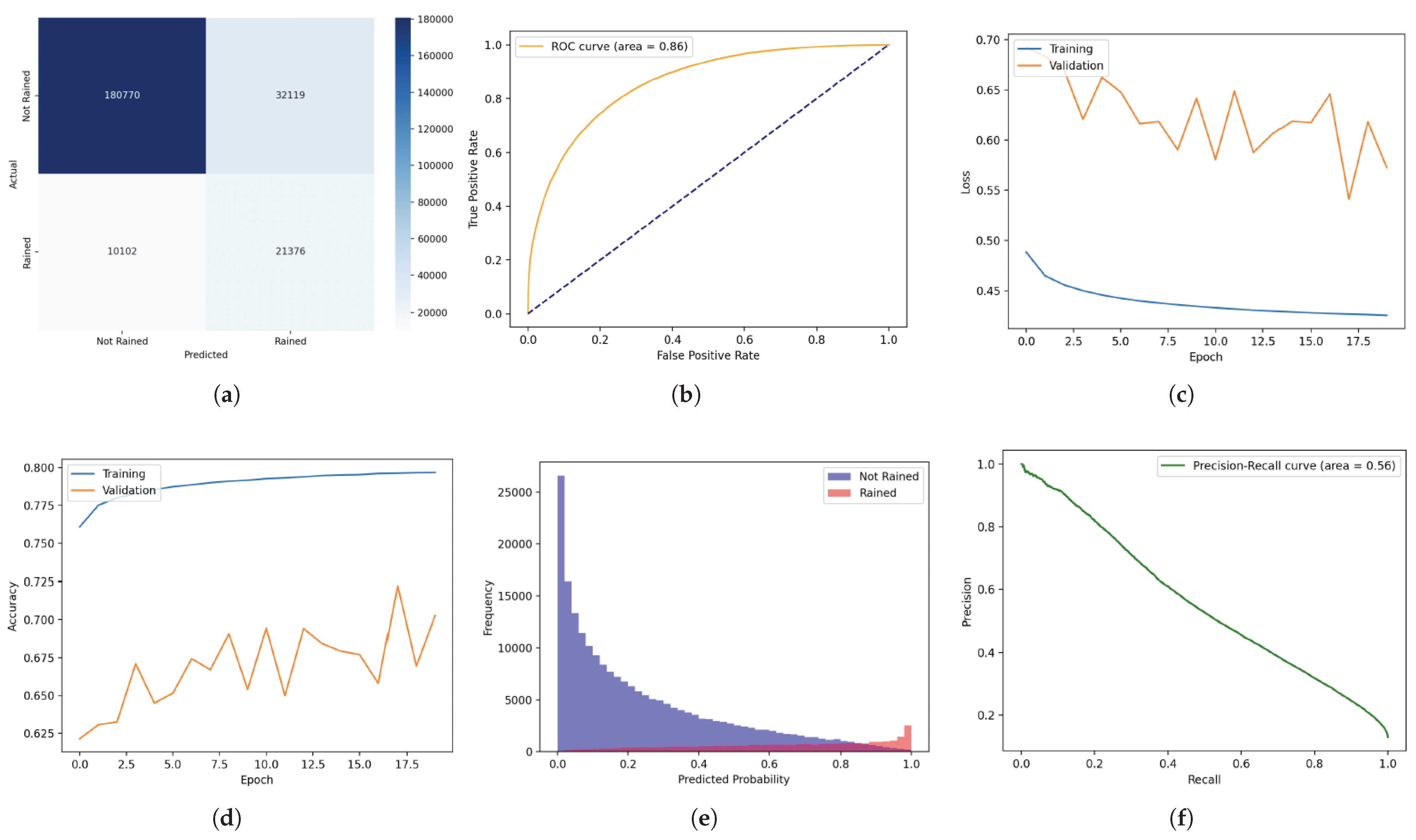
• Confusion Matrix: The deep learning model’s confusion matrix (see Figure 3a) reveals a significant improvement in identifying true positives for rain events compared to previous models. While the model demonstrates high accuracy, the occurrence of false positives— instances predicted as rain that did not actually result in rainfall—warrants further attention and optimization.
• ROC Curve: The model’s ROC curve (see Figure 2b) achieved an AUC of 0.86, illustrating an excellent ability to discriminate between rainy and non-rainy days. This superior AUC value, relative to the machine learning model, underscores the deep learning model’s refined prediction capabilities.

Model Training Dynamics

• Training vs. Validation Loss and Accuracy: Throughout the training epochs, we observed the model’s learning progression through its decreasing loss and stabilizing accuracy (see Figure 3c,d. Despite fluctuations in the validation metrics, indicative of the model’s responsiveness to the data’s complexity, there was a notable convergence in training loss, suggesting effective learning.

Model Predictive Performance

Our deep learning model’s capability extends beyond mere accuracy metrics, as depicted in the Prediction Distribution graph (see Figure 3e). This histogram illustrates the frequency of predicted probabilities for rain events. Notably, there’s a distinct peak at the lower probabilities for ‘Not Rained’, which gradually tapers off, whereas there’s a smaller peak for ‘Rained’ at higher probabilities. This distribution suggests that the model confidently assigns higher probabilities to true rain events and lower probabilities to nonrain events, though there’s a long tail of uncertainty in the ‘Not Rained’ predictions.

Precision and Recall Trade-Off

The Precision-Recall curve (see Figure 3f) with an area of 0.56 further elucidates the balance our model strikes between precision and recall. The model shows a moderate level of precision across different levels of recall, which is particularly useful when considering the cost-sensitive nature of false positives and false negatives in weather forecasting. The area under the curve indicates the model’s average precision across all thresholds and is a useful metric when comparing models where the positive class (rain events) is much less prevalent.

The deep learning model’s nuanced understanding of complex, non-linear relationships in the data culminates in its robust predictive performance. The significant recall improvement is particularly noteworthy, as it indicates a promising direction for future models to deliver even more reliable rain predictions. Nonetheless, the challenge of false positives remains, suggesting potential avenues for refinement, such as exploring different network architectures or introducing regularization techniques to improve model generalization.

5. Conclusions

This paper embarked on an ambitious journey to bridge the significant data divide affecting weather forecasting in remote regions, leveraging the transformative power of artificial intelligence (AI) to illuminate the path forward. Through meticulous research and sophisticated AI modeling, including machine learning and deep learning techniques, this paper demonstrated that it is indeed possible to significantly enhance the accuracy and reliability of weather predictions in areas traditionally handicapped by sparse historical data. The investigation revealed the critical importance of comprehensive datasets enriched with multifaceted parameters for improving model performance. By evaluating the potential of AI to utilize data from welldocumented regions, this paper hypothesized that similar predictive capabilities could be extended to lesserdocumented areas. The results confirmed our hypothesis, showing a notable improvement in predictive accuracy, thereby underscoring the viability of AI in democratizing access to reliable weather forecasting. The implications of our findings are profound, offering a beacon of hope for regions vulnerable to the adverse impacts of weather phenomena. Improved forecasting accuracy holds the promise of better preparedness for extreme weather events, enhanced agricultural planning, and more informed disaster management strategies. This research not only highlights the current challenges in meteorological data availability in India’s remote locales but also showcases the untapped potential of AI to transform weather forecasting into a more inclusive, accurate, and accessible tool for all. However, our journey does not end here. The limitations encountered, notably the challenge of integrating and accurately modeling with sparse data, pave the way for future work. Our proposed direction for advancing this field involves the exploration of new data sources, the integration of additional relevant features, and the continual refinement of AI models. By pushing the boundaries of current methodologies and embracing the complexity of diverse climatic conditions, we stand on the brink of unlocking even more sophisticated and nuanced forecasting models. In conclusion, this research represents a significant step forward in the quest to enhance weather forecasting capabilities in remote regions. By harnessing the power of AI, we have laid the groundwork for future advancements that promise to make accurate weather predictions accessible to all corners of India, regardless of their data richness. As we look to the horizon, it is clear that the integration of technology and innovative scientific approaches will continue to play a pivotal role in our ongoing battle against the unpredictability of weather, ultimately contributing to a safer, more resilient, and wellprepared society. This paper is a testament to the ingenuity of modern computational methods in tackling real-world challenges and a call to action for researchers, policymakers, and technologists to collaborate in harnessing the full potential of AI for the betterment of humanity’s interaction with the natural world.

References

1. Baer, F. Numerical weather prediction. Adv. Comput. 2000, 52, 91–157. [Google Scholar] [CrossRef]
2. Brotzge, J.A.; Berchoff, D.; Carlis, D.L.; Carr, F.H.; Carr, R.H.; Gerth, J.J.; Gross, B.D.; Hamill, T.M.; Haupt, S.E.; Jacobs, N.; et al. Challenges and Opportunities in Numerical Weather Prediction. Bull. Meteorol. Soc. 2023, 104, E698–E705. [Google Scholar] [CrossRef]
3. Rasp, S.; Dueben, P.D.; Scher, S.; Weyn, J.A.; Mouatadid, S.; Thuerey, N. WeatherBench: A Benchmark Data Set for Data-Driven Weather Forecasting. J. Adv. Model Earth Syst. 2020, 12, 203. [Google Scholar] [CrossRef]
4. Cressman, G.P. Numerical Weather Prediction in daily use. Sci. New Ser. 1965, 148, 319–327. [Google Scholar] [CrossRef] [PubMed]
5. Robertson, D.E.; Shrestha, D.L.; Wang, Q.J. Post-processing rainfall forecasts from numerical weather prediction models for short-term streamflow forecasting. Hydrol. Earth Syst. Sci. 2013, 17, 3587–3603. [Google Scholar] [CrossRef]
6. Foemko, A.A. Numerical Method for Weather Forecasting Problem. EOLSS. 2022. Available online: https://www.eolss.net/sample-chapters/C02/E6-04-05-05.pdf (accessed on 10 October 2024).
7. Hollingsworth, A.; Viterbo, P.; Simmons, A.J. The Relevance of Numerical Weather Prediction for Forecasting Natural Hazards and for Monitoring the Global Environment. 2002. Available online: https://www.ecmwf.int/sites/default/files/elibrary/2002/9989-relevance-numerical-weather-prediction-forecasting-natural-hazards-and-monitoring-global.pdf (accessed on 10 October 2024).
8. Basu, A.; Halder, A. Importance of Numerical Weather Prediction in Variable Renewable Energy Forecast. 2017. Available online: https://regridintegrationindia.org/wp-content/uploads/sites/3/2017/09/6B_5_GIZ17_164_paper_Abhijit_Basu.pdf (accessed on 10 October 2024).
9. Schulze, G.C. Atmospheric observations and numerical weather prediction. S. Afr. J. Sci. 2007, 103, 318–323. [Google Scholar]
10. Molnar, C. Interpretable Machine Learning: A Guide for Making Black Box Models Explainable. Available online: https://christophm.github.io/interpretable-ml-book/ (accessed on 10 October 2024).
11. Bochenek, B.; Ustrnul, Z. Machine Learning in Weather Prediction and Climate Analyses—Applications and Perspectives. Atmosphere 2022, 13, 180. [Google Scholar] [CrossRef]
12. Tandon, S.; Patel, A.; Singh, P.K. Weather Prediction Using Machine Learning. 2021. Available online: https://ssrn.com/abstract=3836085 (accessed on 12 February 2021).
13. Singh, S.; Kaushik, M.; Gupta, A.; Malviyaanilkmalviya, A.K. Weather Forecasting Using Machine Learning Techniques. 2019. Available online: https://ssrn.com/abstract=3350281 (accessed on 11 March 2019).
14. Haque, S.; Eberhart, Z.; Bansal, A.; McMillan, C. Semantic Similarity Metrics for Evaluating Source Code Summarization. In Proceedings of the IEEE International Conference on Program Comprehension, IEEE Computer Society, Virtual, 16–17 May 2022; pp. 36–47. [Google Scholar] [CrossRef]
15. Jayasingh, S.K.; Mantri, J.K.; Pradhan, S. Smart Weather Prediction Using Machine Learning; Lecture Notes in Networks and Systems; Springer Science and Business Media Deutschland GmbH: Berlin/Heidelberg, Germany, 2022; pp. 571–583. [Google Scholar] [CrossRef]
16. Hemalatha, G.; Rao, K.S.; Kumar, D.A. Weather Prediction using Advanced Machine Learning Techniques. Phys. Conf. Ser. 2021, 2089, 012059. [Google Scholar] [CrossRef]
17. Hanoon, M.S.; Ahmed, A.N.; Zaini, N.A.; Razzaq, A.; Kumar, P.; Sherif, M.; Sefelnasr, A.; El-Shafie, A. Developing machine learning algorithms for meteorological temperature and humidity forecasting at Terengganu state in Malaysia. Sci. Rep. 2021, 11, 18935. [Google Scholar] [CrossRef]
18. Oshodi, I. Machine learning-based algorithms for weather forecasting. Int. J. Artif. Intell. Mach. Learn 2022, 2, 12–20. [Google Scholar] [CrossRef]
19. Fowdur, T.P.; Nassir-Ud-Diin, I.N.R.M. A real-time collaborative machine learning based weather forecasting system with multiple predictor locations. Array 2022, 14, 100153. [Google Scholar] [CrossRef]
20. Rahman, M.S.; Tumpa, F.A.; Islam, M.S.; Arabi, A.A.; Hossain, M.S.B.; Haque, M.S.U. Comparative Evaluation of Weather Forecasting using Machine Learning Models. arXiv 2024, arXiv:2402.01206. [Google Scholar]
21. Brownlee, J. Deep Learning for Time Series Forecasting: Predict the Future with MLPs, CNNs and LSTMs in Python; Machine Learning Mastery: Melbourne, Australia, 2018. [Google Scholar]
22. Hyndman, R.J.; Athanasopoulos, G. Forecasting: Principles and Practice; OTexts: Clayton, Australia, 2018. [Google Scholar]
23. Zenkner, G.; Navarro-Martinez, S. A flexible and lightweight deep learning weather forecasting model. Appl. Intell. 2023, 53, 24991–25002. [Google Scholar] [CrossRef]
24. Kumar, A.; Sharma, S. Deep Learning Approaches for Weather Forecasting: A Comprehensive Review. Int. J. Comput. Appl. 2020, 177, 20–26. [Google Scholar]
25. Gong, B.; Langguth, M.; Ji, Y.; Mozaffari, A.; Stadtler, S.; Mache, K.; Schultz, M.G. Temperature forecasting by deep learning methods. Geosci. Model Dev. 2022, 15, 8931–8956. [Google Scholar] [CrossRef]
26. Schultz, M.G.; Betancourt, C.; Gong, B.; Kleinert, F.; Langguth, M.; Leufen, L.H.; Leufen, L.H.; Stadtler, A.M.S. Can deep learning beat numerical weather prediction? Philos. Trans. R. Soc. Math. Phys. Eng. Sci. 2021, 379, 2194. [Google Scholar] [CrossRef]
27. Ren, X.; Li, X.; Ren, K.; Song, J.; Xu, Z.; Deng, K.; Wang, X. Deep Learning-Based Weather Prediction: A Survey. Big Data Res. 2021, 23, 100178. [Google Scholar] [CrossRef]
28. Espeholt, L.; Agrawal, S.; Sønderby, C.; Kumar, M.; Heek, J.; Bromberg, C.; Gazen, C.; Carver, R.; Andrychowicz, M.; Kalchbrenner, N.; et al. Deep learning for twelve hour precipitation forecasts. Nat. Commun. 2022, 13, 1–10. [Google Scholar] [CrossRef]
29. Weyn, J.A.; Durran, D.R.; Caruana, R. Improving Data-Driven Global Weather Prediction Using Deep Convolutional Neural Networks on a Cubed Sphere. J. Adv. Model Earth Syst. 2020, 12, 2109. [Google Scholar] [CrossRef]
30. Universitas Indonesia. In Proceedings of the ICACSIS 2015:2015 International Conference on Advanced Computer Science and Information Systems, Depok, Indonesia, 10–11 October 2015.
31. Roy, D.S. Forecasting the Air Temperature at a Weather Station Using Deep Neural Networks. In Procedia Computer Science; Elsevier: Amsterdam, The Netherlands, 2020; pp. 38–46. [Google Scholar] [CrossRef]
32. Hewage, P.; Trovati, M.; Pereira, E.; Behera, A. Deep learning-based effective fine-grained weather forecasting model. Pattern Anal. Appl. 2021, 24, 343–366. [Google Scholar] [CrossRef]
33. Grönquist, P.; Yao, C.; Ben-Nun, T.; Dryden, N.; Dueben, P.; Li, S.; Hoefler, T. Deep learning for post-processing ensemble weather forecasts. Philos. Trans. R. Soc. 2021, 379, 20200092. [Google Scholar] [CrossRef]
34. Li, X.; Zhang, Y. Large Language Models in Weather Forecasting: Opportunities and Challenges. J. Artif. Intell. Weather. 2021, 38, 450–465. [Google Scholar]
35. Suthar, T.; Shah, T.; Raja, M.K.; Raha, S.; Kumar, A.; Ponnusamy, M. Predicting Weather Forecast Uncertainty based on Large Ensemble of Deep Learning Approach. In Proceedings of the International Conference on Self Sustainable Artificial Intelligence Systems, ICSSAS 2023—Proceedings, Institute of Electrical and Electronics Engineers Inc., Erode, India, 18–20 October 2023; pp. 340–345. [Google Scholar] [CrossRef]
36. He, H.; Garcia, E.A. Learning from Imbalanced Data. IEEE Trans. Knowl. Data Eng. 2009, 21, 1263–1284. [Google Scholar]
37. Chang, C.; Wang, W.-Y.; Peng, W.-C.; Chen, T.-F. LLM4TS: Aligning Pre-Trained LLMs as Data- Efficient Time-Series Forecasters. arXiv 2023, arXiv:2308.08469. [Google Scholar] [CrossRef]
38. Jin, M.; Zhang, Y.; Chen, W.; Zhang, K.; Liang, Y.; Yang, B.; Wen, Q. Position Paper: What Can Large Language Models Tell Us about Time Series Analysis. preprint 2024, arXiv:2402.02713. [Google Scholar]
39. Jin, M.; Zhang, Y.; Chen, W.; Zhang, K.; Liang, Y.; Yang, B.; Jindong, W.; Shirui, P.; Qingsong, W. Time-LLM: Time Series Forecasting by Reprogramming Large Language Models. Available online: https://openreview.net/forum?id=Unb5CVPtae (accessed on 10 October 2024).
40. Jones, L.; Brown, M. Advancements in AI for Weather Prediction. Weather. Clim. 2019, 12, 112–128. [Google Scholar]
41. Gupta, R.; Patel, S. Generative AI for Weather Data Analysis. IEEE Trans. Neural Netw. 2017, 29, 2100–2113. [Google Scholar]
42. Bihlo, A. A generative adversarial network approach to (ensemble) weather prediction. Neural Netw. 2021, 139, 1–16. [Google Scholar] [CrossRef]
43. Li, L.; Carver, R.; Lopez-Gomez, I.; Sha, F.; Anderson, J. Generative Emulation of Weather Forecast Ensembles with Diffusion Models. 2024. Available online: https://www.science.org (accessed on 10 October 2024).
44. Bilgin, O.; Mąka, P.; Vergutz, T.; Mehrkanoon, S. TENT: Tensorized Encoder Transformer for Temperature Forecasting. arXiv 2021, arXiv:2106.14742. [Google Scholar]
45. Olarewaju, I.K.; Kim, K.K. Development of a Weather Prediction Device Using Transformer Models and IoT Techniques. J. Sens. Sci. Technol. 2022, 32, 164–168. [Google Scholar] [CrossRef]
46. Alerskans, E.; Nyborg, J.; Birk, M.; Kaas, E. A transformer neural network for predicting near-surface temperature. Meteorol. Appl. 2022, 29, 2098. [Google Scholar] [CrossRef]
47. Cachay, S.R.; Mitra, P.; Hirasawa, H.; Kim, S.; Hazarika, S.; Hingmire, D.; Rasch, P.; Singh, H.; Singh, K. ClimFormer-A Spherical Transformer Model for Long-term Climate Projections. In Proceedings of the Machine Learning and the Physical Sciences Workshop, NeurIPS 2022, New Orleans, LA, USA, 3 December 2022. [Google Scholar]
48. Available online: https://www.kaggle.com/datasets/selfishgene/historical-hourly-weather-data/data (accessed on 10 October 2024).
49. Ministry of Earth Sciences, Government of India. Climatic Classifications and Monthly Weather Reports. 2022. Available online: http://moes.gov.in/climate_data.html. (accessed on 10 October 2024).
50. García, S.; Luengo, J.; Herrera, F. Data Preprocessing in Data Mining; Springer International Publishing: Berlin/Heidelberg, Germany, 2015. [Google Scholar]
51. Zheng, A.; Casari, A. Feature Engineering for Machine Learning: Principles and Techniques for Data Scientists; O’Reilly Media: Newton, MA, USA, 2018. [Google Scholar]
52. Provides Comprehensive Guides and Examples for Machine Learning Models, Preprocessing, and Model Evaluation.TensorFlow Documentation. Available online: https://www.tensorflow.org/guide (accessed on 10 October 2024).
53. World Meteorological Organization. Advances in Weather Data Collection and Analysis: A Comprehensive Review; WMO Technical Report; World Meteorological Organization: Geneva, Switzerland, 2021; Volume 567, pp. 1–50. [Google Scholar]
54. Sharma, K.; Singh, P. Challenges in Weather Data Availability for Remote Areas in India. Environ. Res. Lett. 2020, 15, 034010. [Google Scholar] [CrossRef]
55. India Meteorological Department. Data Supply Portal: Access and Limitations. 2023. Available online: https://www.india.gov.in/website-data-supply-portal (accessed on 10 October 2024).
56. James, G.; Witten, D.; Hastie, T.; Tibshirani, R. An Introduction to Statistical Learning: With Applications in R; Springer: Berlin/Heidelberg, Germany, 2013. [Google Scholar]
57. Chollet, F. Deep Learning with Python; Manning Publications: Shelter Island, NY, USA, 2017. [Google Scholar]
58. Kumar, R.; Gupta, A. Impact of Historical Weather Data Availability on Weather Forecasting: A Case Study of Remote Cities in India. J. Remote. Sens. Clim. Stud. 2019, 25, 112–120. [Google Scholar]
Figure 1. Process Diagram.
Atmosphere 16 00587 g001
Figure 2. (a) Confusion Matrix. (b) Receiver Operating Characteristic (ROC) Curve.
Atmosphere 16 00587 g002
Figure 3. (a) Confusion Matrix for the Deep Learning Model. (b) ROC Curve for the Deep Learning Model. (c) Model Loss Over Epochs for the Deep Learning Model. (d) Model Accuracy Over Epochs for the Deep Learning Model. (e) Prediction Distribution-Deep Learning Model. (f) Precision-Recall Curve-Deep Learning Model.
Atmosphere 16 00587 g003
Disclaimer/Publisher’s Note: The statements, opinions and data contained in all publications are solely those of the individual author(s) and contributor(s) and not of MDPI and/or the editor(s). MDPI and/or the editor(s) disclaim responsibility for any injury to people or property resulting from any ideas, methods, instructions or products referred to in the content.