Diffusion-Model-Based Downscaling of Observed Sea Surface Height over the Kuroshio Extension Since 2000

Abstract

Satellite altimetry measurements enable the resolution of ocean variability from basin-scale to mesoscale. However, the spatial resolution is still limited. The two-dimensional map from the merged data for all the available altimetry satellites can resolve mesoscale eddies down to 150 km in mid-latitudes, for example. We introduce a generative diffusion model to downscale a merged altimetry dataset, which is applied to the eddy-rich Kuroshio Extension region from 2000 to 2022. A reanalysis dataset with a high-resolution model at a horizontal scale of approximately 12 km is employed to train the diffusion model. Using the trained generative diffusion model, the merged dataset at a grid size of 1/4° is downscaled. It was demonstrated that this trained generative diffusion model outperforms the other two high-resolution reanalyses and neural-network-based datasets. The downscaled data reproduce the spatial patterns and power spectra of satellite along-track measurements. The analysis also indicates that eddy kinetic energy at horizontal scales less than 250 km has intensified by 10.14 cm²/s² (2.07%) per decade since 2004 in the Kuroshio Extension region. Our results underscore the potential of generative diffusion models in downscaling satellite altimetry datasets and improving our understanding of ocean dynamics at mesoscales.

1. Introduction

Satellite altimeters have significantly improved our understanding of sea surface height (SSH) variations on a global scale over the past four decades. Advances in ocean dynamics during the past decades relied heavily on satellite altimetry datasets [1,2,3]. However, the spatial resolution of current nadir-looking altimeters is limited by the presence of large gaps between satellite tracks [4,5]. Generally, along-track SSH can resolve ocean waves with typical wavelengths down to 70 km while the spatial resolution in a two-dimensional gridded SSH map is only on the order of 150 km [3,6], inadequate for resolving mesoscale and submesoscale processes, which have a scale down to ~1 km. Although optimal interpolation, data assimilation, and the other merging algorithm of multi-satellite altimeter data continue to be optimized to fill the gaps between satellite tracks [7,8,9,10,11,12,13], the resolution of a two-dimensional gridded SSH map cannot be increased due to a limited number of altimetry satellites.

High-resolution global and regional ocean models have been developed to improve the horizontal resolution of SSH maps and downscaling is used to generate SSH maps of a higher resolution, also referred to as super-resolution (SR). Downscaling through dynamic model simulations is physics-based but comes with substantial computational cost [14,15]. On the other hand, traditional statistical downscaling methods reduce computational demands but struggle with unlearned data relationships and distributions [16,17,18]. Deep-learning-based methods have emerged as a new paradigm for satellite altimetry data downscaling. This approach is data-driven and often outperforms traditional dynamical and statistical downscaling algorithms [4,19,20,21,22]. Recently, generative diffusion models (DMs) have become a cutting-edge technique for image super-resolution [23,24,25,26] and climate downscaling [27,28,29,30,31].

The importance of SSH downscaling stems not only from the sparse horizontal resolution of satellite altimetry datasets but also from the profound impacts of ocean eddies on large-scale ocean circulation [2,32], heat uptake [33], marine ecosystem [34], and climate change [35,36]. Mesoscale ocean eddies with sizes of 100–250 km contain 80% of the total ocean kinetic energy [37]. In addition, the role of mesoscale processes at scales smaller than 100 km has been overlooked due to the low effective resolution of satellite observations. Using high-resolution ocean simulations, recent studies have suggested that such mesoscale processes are crucial for upper ocean heat transport [2,38,39] and El Niño-Southern Oscillation [40].

In this study, we developed a state-of-the-art generative DM to successfully downscale traditional AVISO observational SSH data from 2000 onwards in the eddy-rich Kuroshio Extension region, which is an ideal test-bed for high-resolution SSH mapping. Despite the lack of observational high-resolution SSH data, we leveraged model reanalysis outputs to extract fine-scale SSH information from coarse satellite observations. We further tested the limits of our diffusion model by manipulating the input reanalysis SSH data in several hypothetical scenarios. Our newly generated dataset reveals an intensification trend in ocean eddies over the past two decades in the Kuroshio Extension region.

2. Datasets and Methods

2.1. Datasets

For gridded satellite observations, we used daily SSH from the Archiving, Validation and Interpretation of Satellite Oceanographic (AVISO) data of the Copernicus Marine Environment Monitoring Service (CMEMS) with a horizontal resolution of 0.25° from 2000 to 2022.

For satellite along-track SSH observations, we used multiple satellites passing over the Kuroshio Extension region. The data were partly processed by the Data Unification and Altimeter Combination System (DUACS) multimission altimeter data processing system. The satellites included Jason 3, Sentinel 3A, Sentinel 3B, HY 2B, and Sentinel 6 in the DUACS. Specifically, we used the unfiltered, daily Level 3 sea level anomaly observations. At Level 3, the observations have been corrected for atmospheric effects, the barotropic tide has been removed, and the data have been adjusted to ensure consistency between the different altimeter missions. Satellite along-track observations cover the period from 1 December 2020 to 31 December 2022.

For high-resolution SSH reanalysis datasets, we used the daily SSH from the CMEMS global ocean eddy-resolving (1/12° horizontal resolution) reanalysis (GLORYS12) covering the period from 1 July 2020 to 31 January 2024 [41]. We further utilized the daily data-assimilative HYbrid Coordinate Ocean Model (HYCOM) with a horizontal resolution of 1/12° [42].

2.2. Methods

2.2.1. Diffusion Models

The generative DMs were inspired by non-equilibrium thermodynamics [43]. The model contains a forward diffusion process and a reverse denoising process. The forward diffusion process transforms samples from the data distribution $\mathbf{x}\left(0\right)~p\left(\mathbf{x};{\sigma }_{data}\right)$ to that of pure Gaussian noise $\mathbf{x}\left(\mathrm{T}\right)~N\left(0,\mathsf{\sigma }\mathrm{I}\right)$, which can be represented by the stochastic differential equation (SDE). Following Song et al. [24], the SDE for such a process is given by:

$$d\mathbf{x}=f\left(\mathbf{x},t\right)dt+g\left(t\right)dw$$

(1)

where $f\left(\mathbf{x},t\right)$ is the drift coefficient, $g\left(t\right)$ is the diffusion coefficient, and $\mathrm{w}$ is a Wiener process. If the SDE can be reversed, we can use it to generate samples from $p\left(\mathbf{x}\left(0\right)\right)$. The reverse denoising SDE process is:

$$d\mathbf{x}=[f\left(\mathbf{x},t\right)-{g\left(t\right)}^2{\mathsf{\nabla }}_{\mathbf{x}}log{p}_t(\mathbf{x})]dt+g(t)d\overline{\mathit{w}}$$

(2)

where $\overline{\mathit{w}}$ is a Wiener process with time flowing backwards from T to 0. ${\mathsf{\nabla }}_{\mathbf{x}}log{p}_t\left(\mathbf{x}\right)$ is the score function, a vector that denotes the gradient of the log probability density function of the data distribution.

We can also begin by examining the deterministic ordinary differential equation (ODE). The reverse ODE process is then as follows:

$$d\mathbf{x}=[f\left(\mathbf{x},t\right)-{\displaystyle \frac{1}{2}}{g\left(t\right)}^2{\mathsf{\nabla }}_{\mathbf{x}}log{p}_t(\mathbf{x})]dt$$

(3)

Following Karras et al. [25], the ODE can also be written as:

$$d\mathbf{x}=[{\displaystyle \frac{\dot{s}\left(t\right)}{s\left(t\right)}}\mathbf{x}-{s\left(t\right)}^2\dot{\sigma }(t)\sigma (t){\mathsf{\nabla }}_{\mathbf{x}}logp({\displaystyle \frac{\mathbf{x}}{s\left(t\right)}};\sigma (t))]dt$$

(4)

where $s\left(t\right)$ is the scaling factor. Thus, the reverse ODE mainly focuses on the reparameterization of $s\left(t\right)$ and $\sigma \left(t\right)$. In addition, unlike traditional DMs (i.e., DDPM and DDIM), the diffusion and denoising processes can be simplified as adding or subtracting Gaussian noise with varying intensities (different standard deviations [25]). Thus, $\sigma \left(t\right)=t$ in our diffusion model. We use 182 time steps during evaluation but find that using just 100 is sufficient for a similar accuracy. Specifically, the diffusion model was trained in parallel on three NVIDIA RTX 3070 GPUs (Santa Clara, CA, USA) using data from 1 July 2020, to 31 January 2024. Due to GPU memory constraints, we used a batch size of 2 and employed gradient accumulation over 5 steps to effectively increase the batch size during optimization. Each epoch of training took approximately 0.8 h. During inference, a single NVIDIA RTX 3070 GPU was used and generating one SSH snapshot required about 50 s.

2.2.2. U-Net and SR Generative Adversarial Network (SR-GAN)

In this study, we utilize the U-Net in our diffusion model. The U-Net architecture, originally introduced by Ronneberger et al. [44], follows a symmetric encoder–decoder structure with skip connections that link each encoding layer to its corresponding decoding layer. These skip connections allow fine-resolution features to be retained and directly reused during upsampling, which is particularly advantageous for preserving mesoscale and submesoscale patterns in SSH data. In our implementation, the U-Net is trained by minimizing the Mean Squared Error (MSE) between the U-Net predicted image and the samples from the data.

The SR-GAN network is consistent with the previous paper [45]. The VGG19 network used in perceptual loss is mainly for extracting high-level image features to better measure the similarity between the generated image and the original high-resolution image [46]. More details and a comparison will be shown in Section 3.2.

2.2.3. Kuroshio Extension SSH Downscaling Diffusion Model

In this study, the Kuroshio Extension region is defined as the area between 27–41.22° N and 140–168.44° E. Due to the fact that the diffusion model requires the grid points must be powers of 2, we interpolate the GLORYS12 and HYCOM high-resolution reanalyses to a 1/16° resolution using bicubic interpolation.

Since we utilize a conditional diffusion model, an additional input of a low-resolution image is required for SSH downscaling. However, after interpolating the 1/16° GLORYS12 ocean model reanalysis data to 1/4°, the resulting images still contain more details than the original 0.25° AVISO data. Thus, the 1/16° high-resolution GLORYS12 data are first spline-interpolated to 0.5° low-resolution data. These high- and low-resolution GLORYS12 datasets are then included in the training set to develop an 8-fold downscaling model. For the Kuroshio Extension region, a 1/16° resolution corresponds to 512 grid points in the zonal direction and 256 grid points in the meridional direction. The 0.5° resolution thus should be 64 grid points in the zonal direction and 32 grid points in the meridional direction.

The sample time range for the training set is from 1 July 2020 to 31 July 2023 while the validation set includes March 2018, June 2019, September 2023, and January 2024. The sample time range for the validation set is not included in the training set.

When applying our model to AVISO observations, we first spline-interpolate the AVISO data to a 0.5° resolution and then perform 8-fold downscaling to 1/16°. We will further show the structure of our diffusion model in Section 3.

2.2.4. Metrics for Different Model Comparison

We calculate six metrics to compare and evaluate different downscaling algorithms, including the Peak Signal-to-Noise Ratio (PSNR), Structure Similarity Index Measure (SSIM), Mean Absolute Error (MAE), Root Mean Square Error (RMSE), Temporal Correlation Coefficient (TCC), and Pattern Correlation Coefficient (PCC). Their definitions are as follows:

$$PSNR={\displaystyle \frac{1}{n}}\sum _{i=1}^{n}10\times {log}_{10}\left({\displaystyle \frac{{C_{max}}^2}{MSE}}\right)$$

(5)

$$MSE={\displaystyle \frac{1}{n}}\sum _{i=1}^n{\left(h_i-h_i^{\prime }\right)}^2$$

(6)

$$SSIM={\displaystyle \frac{1}{n}}\sum _{i=1}^n{\displaystyle \frac{(2{\mu }_i{\mu }_i^{\prime }+C_1)(2{\sigma }_i{\sigma }_i^{\prime }+C_2)}{({({\mu }_i)}^2+{({\mu }_i^{\prime })}^2+C_1)({\left({\sigma }_i\right)}^2+{({\sigma }_i^{\prime })}^2+C_2)}}$$

(7)

$$MAE={\displaystyle \frac{1}{n}}\sum _{i=1}^n\left|h_i-h_i^{\prime }\right|$$

(8)

$$RMSE=\sqrt{{\displaystyle \frac{1}{n}}\sum _{i=1}^n{\left(h_i-h_i^{\prime }\right)}^2}$$

(9)

Here, $n$ represents the total number of sample days in the validation set. $h_i$ and $h_i^{\prime }$ denote the GLORYS12 high-resolution reanalysis and the downscaling outputs, respectively. ${\mu }_i$ and ${\mu }_i^{\prime }$ represent the spatial means of $h_i$ and $h_i^{\prime }$ while ${\sigma }_i$ and ${\sigma }_i^{\prime }$ represent spatial standard deviations. $C_{max}$ denotes the maximum value of the daily SSH and equals 3. $C_1$ and $C_2$ are constants to avoid computation instability when the denominator approaches zero.

TCC is defined as the temporal correlation coefficient of $h_i$ and $h_i^{\prime }$ at the same non-land grid points, followed by averaging the correlation coefficients across these non-land points. PCC is the spatial correlation coefficient of $h_i$ and $h_i^{\prime }$ for each day, followed by averaging over $\mathrm{n}$ days.

2.2.5. 2-Dimensional (2D) Fourier Transforms and Power Spectrum Analysis

To calculate the power spectra of various datasets, we utilize a 2D discrete fast Fourier transform (2DFFT). To focus on the regional scale variability, we first kick off the land points, followed by subtracting the zonal mean from the SSH data. As suggested by Sasaki et al. [40], the zonal mean values affect scales larger than 300 km.

The calculation steps are as follows: We apply 2DFFT to the daily SSH for the sample period to obtain the power spectra and then average the daily power spectra over the entire sample period. The 2DFFT converts SSH from the spatial domain into the Fourier frequency domain. The 2DFFT of SSH $h(x,y)$ is defined as:

$$H(X,Y)=\sum _{x=0}^{M-1}\sum _{y=0}^{N-1}h(x,y)·e^{-i2\pi (\frac{ux}{M}+\frac{vy}{N})}$$

(10)

where $h(x,y)$ are the input SSH data in the spatial domain. $\mathrm{H}(\mathrm{X},\mathrm{Y})$ is the output signal in the frequency domain. $M$ and $N$ are the dimensions of the input SSH data. $X$ and $Y$ are the frequency components corresponding to the spatial dimensions $x$ and $y$. $i$ is the imaginary unit.

The power spectral density (PSD) represents the distribution of power across different frequency components. The PSD $P(X,Y)$ is given by:

$$P(X,Y)={\left|H(X,Y)\right|}^2$$

(11)

where $\left|H(X,Y)\right|$ is the magnitude of the Fourier coefficients.

To reduce the 2D PSD to a one-dimensional function, radial averaging is performed. This process involves averaging the PSD over concentric circles of constant radius $r$ in the frequency domain. The radius $r$ is defined as:

$$r=\sqrt{X^2+Y^2}$$

(12)

The radially averaged PSD is thus calculated by averaging the $P(X,Y)$ over all points $(X,Y)$ that lie on the circle with the radius $r$.

After doing the above steps, the power spectra for multiple days are averaged to produce the final power spectrum used for analysis.

2.2.6. Error Ratios in Spectral Analysis

In this study, we subtract the daily high-resolution SSH outputs of each model on the validation set from the high-resolution GLORYS12 data, then apply 2DFFT to obtain the power spectrum of the error, and finally divide it by the power spectrum of the GLORYS12 high-resolution data. Therefore, the error ratio indicates the differences between the downscaling model and the input ground truth across different frequencies. Empirically, a ratio greater than 0.5 represents that the downscaling model has significant errors, whereas a ratio less than 0.5 suggests that the model well resembles the ground truth. More details can be found in Ballarotta et al. [6].

2.2.7. Eddy, Submesoscale Variability, Rossby Number (Ro), and Eddy Kinetic Energy (EKE)

In this study, we define eddy-scale variability, encompassing both mesoscale and submesoscale, by high-pass filtering with a cut-off wavelength of 250 km via 2DFFT. Moreover, submesoscale variability is defined as a spatial scale smaller than 50 km via a 2DFFT high-pass filter.

Relative vorticity $\xi$ is defined as the rotational component of horizontal motions:

$$\xi ={\displaystyle \frac{\partial v}{\partial x}}-{\displaystyle \frac{\partial u}{\partial y}}$$

(13)

where $u$ and $v$ are the zonal and meridional velocities.

To derive the $\xi$ from SSH, the $u$ and $v$ are obtained, assuming geostrophic balance under the approximation:

$$u_g=-{\displaystyle \frac{g}{f}}{\displaystyle \frac{\partial h}{\partial y}}$$

(14)

$$v_g={\displaystyle \frac{g}{f}}{\displaystyle \frac{\partial h}{\partial x}}$$

(15)

where $g$ is the acceleration due to gravity and $f$ is the Coriolis parameter (Earth’s rotation rate).

The relative vorticity should be:

$$\xi ={\displaystyle \frac{g}{f}}({\displaystyle \frac{{\partial }^{2}h}{\partial x^2}}+{\displaystyle \frac{{\partial }^{2}h}{\partial y^2}})$$

(16)

The Rossby number $Ro$ is a non-dimensional number utilized to represent the surface frontal structure [38]. It is defined as $Ro=\xi /f$. When this non-dimensional number is larger than 0.1, the ocean eddies may be large [47,48,49].

The kinetic energy, KE, is calculated from the surface geostrophic current maps:

$$KE={\displaystyle \frac{1}{2}}(u_g^2+v_g^2)$$

(17)

The eddy kinetic energy, EKE, is defined as the time-varying component of the KE using a Reynolds decomposition:

$$EKE={\displaystyle \frac{1}{2}}(\overline{{u^{\prime }}^2}+\overline{{v^{\prime }}^2})$$

(18)

where the constant ocean water density is ignored. $u^{\prime }$ and $v^{\prime }$ represent the eddy-scale or submesoscale velocities via a 2DFFT.

3. Results

3.1. Diffusion-Model-Based Downscaling Using Ocean Reanalysis

Reanalysis products employ state-of-the-art ocean models incorporating data assimilation schemes to produce SSH that is closer to observations [50,51]. We first compare the high-resolution GLORYS12 reanalysis to low-resolution AVISO observations. AVISO captures large-scale ocean circulation; however, due to its coarse resolution, ocean eddies with relative vorticity comparable to Earth’s rotation rate (|Ro| > 0.1) typically appear on the map as isolated centers (Figure 1a,c). In contrast, GLORYS12 reproduces the observed large-scale patterns well while simulating wavy characteristics and filaments of ocean eddies (Figure 1b,d). Cyclonic and anticyclonic eddies are ubiquitous over the Kuroshio Extension region in daily snapshots. On 15 January 2022, AVISO reveals an array of cyclonic and anticyclonic eddies with a southwest–northeast orientation east of the landmass (Figure 1a). While GLORYS12 indeed reproduces these observed eddies, it also spuriously generates northwest–southeast oriented filaments that are absent in the observations for that day (Figure 1b). Similar discrepancies are evident on 1 April 2022, where the cyclonic submesoscale eddy simulated by GLORYS12 is displaced southward (Figure 1d), inconsistent with AVISO observations (Figure 1c).

Given the aforementioned discrepancies, GLORYS12 cannot be treated as the observational ground truth. However, the eddy-scale variability it generates is dynamically constrained by model simulations. Also, its large-scale variability closely resembles observations. Thus, we propose a SSH downscaling scheme for the Kuroshio Extension region based on generative DMs using GLORYS12 reanalysis data, which we term the Kuroshio Extension SSH Downscaling Diffusion Model (KESHDiff, see Section 2.2.1 and Section 2.2.3).

DMs contain a forward diffusion process and a reverse denoising process [23,24] (Figure 2a). As generative models, DMs aim to learn the probability distribution $p\left(\mathbf{x}\right)$ given a set of samples $\left\{\mathbf{x}\right\}$ with standard deviation ${\sigma }_{data}$. The forward diffusion process gradually adds varying levels of independent identically distributed Gaussian noise of standard deviation $\sigma$ to the data to obtain $p\left(\mathbf{x};\sigma \right)$. For ${\sigma }_{max}\gg {\sigma }_{data}$, $p\left(\mathbf{x};{\sigma }_{max}\right)$ is practically similar with pure Gaussian noise, as illustrated by the images from $\mathbf{x}\left(0\right)$ to $\mathbf{x}\left(\mathrm{T}\right)$ in Figure 2a. For the reverse process, the DMs sequentially denoise $\mathbf{x}\left(\mathrm{T}\right)$ back into $\mathbf{x}\left(0\right)$, such that at each noise level, $\mathbf{x}\left(i\right)~p\left({\mathbf{x}}_i;{\sigma }_i\right)$. The endpoint of the reverse process is thus distributed according to the learned data distribution. The above forward diffusion and reverse denoising processes are unconditional, meaning that the generated results are entirely based on the probability distribution learned from the training data. This situation is more akin to an eddy-free run in ocean modeling. In our work, we focus on conditional downscaling with our proposed model, KESHDiff. While KESHDiff’s forward diffusion process is similar to other well-developed DMs, its reverse denoising process incorporates low-resolution data as additional conditions to guide the generation of high-resolution counterparts (Figure 2b). This conditional approach allows for more controlled and targeted generation of high-resolution data. To solve the reverse denoising process in KESHDiff, we utilize a U-Net-like architecture (Figure 2b).

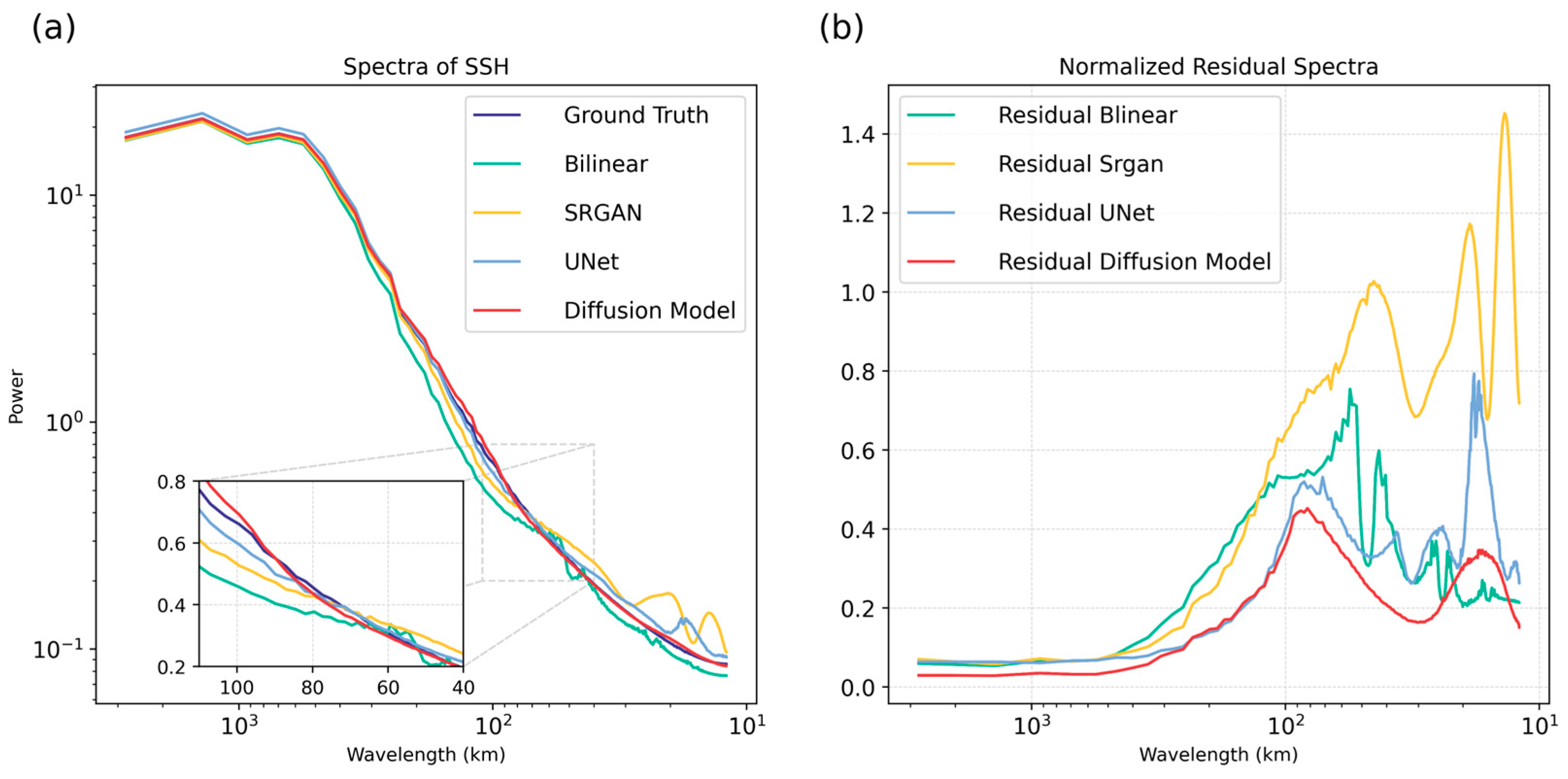
3.2. Model Comparison on the GLORYS12 Validation Set

We comprehensively compare KESHDiff against three other algorithms, including bilinear interpolation, SR-GAN, and U-Net, using the validation set of GLORYS12. KESHDiff outperforms other models across six metrics (

Table 1. Performance of four models across six metrics ¹.

	PSNR (dB)	SSIM	MAE (m)	RMSE	TCC	PCC
Bilinear	50.4494	0.9896	0.0020	0.0030	0.9949	0.9990
SR-GAN	45.8022	0.9797	0.0033	0.0053	0.9970	0.9978
UNet	47.4044	0.9929	0.0040	0.0045	0.9949	0.9996
Diffusion	53.4701	0.9942	0.0015	0.0021	0.9982	0.9996

¹ Parentheses show the units of PSNR and MAE, respectively. The best results are bolded.

), including PSNR, SSIM, MAE, RMSE, TCC, and PCC. Specifically, KESHDiff achieves a PSNR exceeding 53 dB, while bilinear interpolation also surpasses 50 dB, indicating that traditional statistical downscaling methods still retain some efficacy. However, well-trained neural networks like U-Net and KESHDiff demonstrate better performance across multiple metrics. U-Net outperforms bilinear interpolation in terms of SSIM and PCC. In contrast, SR-GAN yields inferior results.

Note that for two-dimensional fields, PSNR, MAE, and RMSE are metrics that quantify the average error across all wavelengths (or scales), thereby focusing on the overall error rather than the error at specific wavelengths. In image signal processing, the long-wavelength components dominate the overall quality of the image and the aforementioned metrics, with the influence of short-wavelength components being almost negligible. However, SSH signals at various wavelengths carry substantial dynamical importance, requiring further assessment in the Fourier space. Figure 3a shows the power spectral density (PSD) of high-resolution SSH from GLORYS12, serving as the ground truth on the validation set, alongside the SSH outputs from four methods. The power spectrum of KESHDiff is indistinguishable from the ground truth across all wavelengths, indicating that the model has effectively learned the spectral characteristics of SSH. The shortest wavelength in the high-resolution data is approximately 12 km, as shown on the x-axis of Figure 3a. Given that we implement an 8-fold downscaling scheme (see Section 2.2.3), the shortest identifiable wavelength for the input low-resolution data (Figure 2b) is only about 96 km. Consequently, the SSH data with wavelengths ranging from 96 km to 12 km are all generated by the models themselves. At wavelengths larger than 500 km, U-Net overestimates the large-scale longwave features while bilinear interpolation underestimates the energy of longwaves. In the wavelength range from 500 km to 60 km, bilinear interpolation, SR-GAN, and U-Net underestimate the energy. At wavelengths shorter than 60 km, bilinear interpolation performs consistently, whereas the other two neural-network-based downscaling schemes inappropriately generate more perturbations.

We also examine the error ratios between these models and the ground truth. The error ratios represent the ratio between the spectra of error and the spectrum of the ground truth across different frequency bands. The error ratios are called the effective spatial resolution, which corresponds to the spatio-temporal scales of the features that can be properly resolved in the two-dimensional maps [6]. From large-scale down to approximately 96 km, the error ratios of three models, excluding SR-GAN, are all less than 0.5, suggesting good performance in capturing large-scale SSH characteristics with relatively small errors (Figure 3b). Among these, KESHDiff exhibits the lowest error ratio, closely resembling the ground truth. In the model-generated wavelength bands, specifically the 96 km to 12 km range, KESHDiff consistently maintains an error ratio below 0.5. U-Net performs well in the 96–20 km range but its error rapidly increases in the shorter wavelength band, indicating artificially enhanced power spectrum energy in this band (Figure 3b). Bilinear interpolation exhibits an even lower ratio than KESHDiff in the 20–12 km range, likely due to smoothing data between grid points, resulting in low power spectrum energy (Figure 3a), rather than being driven by reasonable physical processes.

The surface Rossby number provides an intuitive way to visualize differences between these model results. Figure 4 shows the Rossby number calculated from SSH fields on 1 June 2019. GLORYS12 (serving as ground truth here) reveals highly active mesoscale processes along the Kuroshio main axis and its southern region, along with abundant smaller-scale structures like filaments at eddy edges (Figure 4a). Due to resolution-reducing interpolation, the input field only roughly captures mesoscale processes while completely missing finer structures like filaments (Figure 4b). The results of KESHDiff show that the structure and intensity of mesoscale eddies are very close to the ground truth and the filamentary structures are also essentially consistent with the ground truth, with only minor differences in intensity and shape (Figure 4c). Therefore, it can be considered that KESHDiff generates reasonably small-scale features. The results of U-Net are close to those of KESHDiff but a careful comparison of small-scale features reveals that the filamentary structures of U-Net are not as rich and restored as those of KESHDiff (Figure 4d). SR-GAN, when restoring mesoscale processes, produces striated structures and does not generate small-scale structures, such as filaments (Figure 4e), hence, its performance in the evaluations is inferior to the former two. Traditional interpolation methods are unable to generate reasonable small-scale features (Figure 4f), therefore, they should be used with caution in downscaling processes.

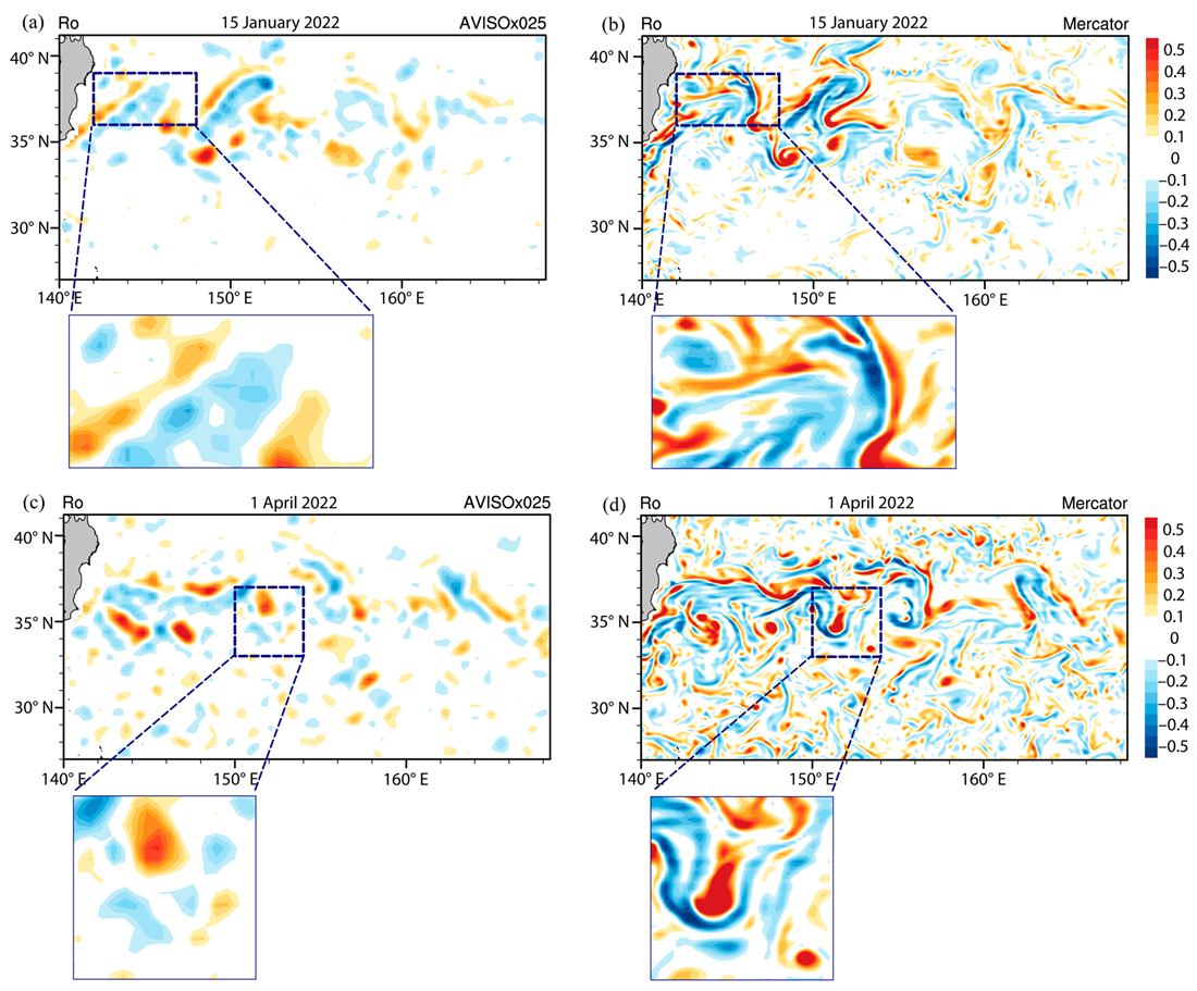
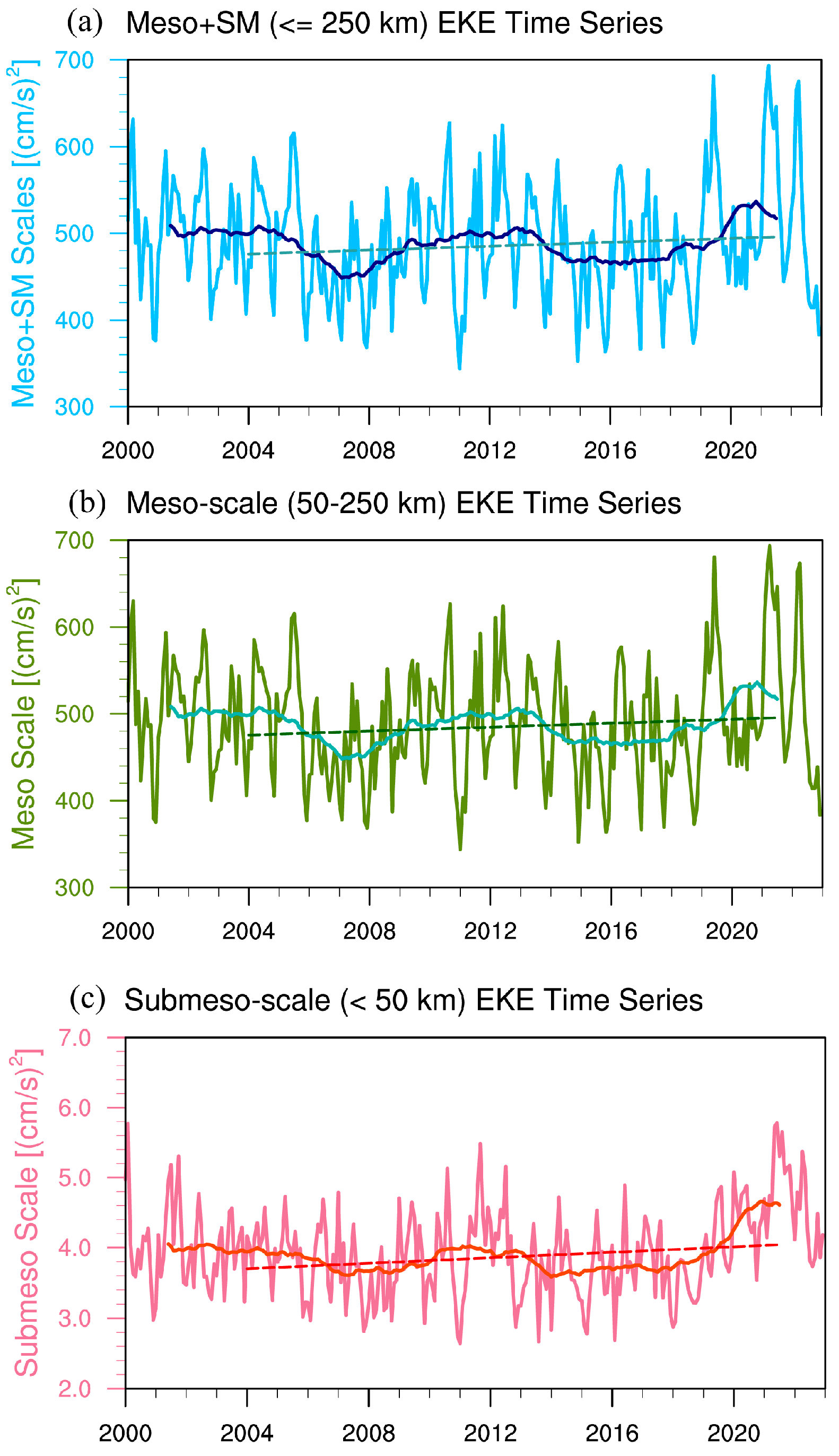
3.3. Application on AVISO and the Intensification of Eddies Since 2004

KESHDiff exhibits exceptional performance in SSH downscaling on the GLORYS12 validation set. Thus, we utilize KESHDiff to downscale the gridded AVISO SSH from a horizontal resolution of 0.25° to 1/16°, achieving a shortest wavelength of approximately 12 km. We compare our KESHDiff output with two sets of high-resolution ocean model reanalysis data assimilating observations (HYCOM and GLORYS12), the original input 0.25° low-resolution AVISO data, and multi-satellite along-track observations. The comparison period spans from 1 December 2020 to 31 December 2022.

The PSD of the along-track observations gradually decreases with shorter wavelengths (Figure 5a), a feature shown in all datasets. HYCOM data perform the worst, exhibiting significant errors compared to the along-track observations at wavelengths exceeding 300 km (Figure 5b). Among the remaining datasets, the discrepancy between KESHDiff and the along-track observations is smallest (Figure 5b).

Surprisingly, although our training set is derived from GLORYS12, our model outperforms GLORYS12 itself when applied to AVISO data. In addition, KESHDiff is also better than the input low-resolution AVISO SSH on large scales. This suggests that ocean reanalysis serves as an effective proxy for direct high-resolution SSH observations in the model training step, despite the unavailability of the latter.

At scales below 300 km, due to the coarse effective spatial resolution, AVISO exhibits a rapid decline in its PSD (Figure 5a). Additionally, the two model reanalyses show consistent declines in PSD compared to KESHDiff. KESHDiff remains the closest to the along-track observations even at the shortest effective wavelength of 70 km (Figure 5b).

Consistent with Figure 1, daily snapshots further demonstrate that KESHDiff has successfully downscaled the SSH over the Kuroshio Extension without generating spurious eddy-scale features (Figure 6). Then, we focus on the long-term changes in eddy-scale EKE over the Kuroshio Extension region. Area-averaged EKE at wavelengths shorter than 250 km exhibits distinct interannual variations (Figure 7a). The EKE was relatively weak during 2015–2016, following the super El Niño, while it intensified during the triple-dip La Niña event of 2020–2022. The 23-year average EKE from 2000 to 2022 is 490.82 cm²/s². Since 2000, the EKE at eddy scales shows a slight but insignificant decreasing trend. However, EKE has significantly intensified since 2004 at a rate of 10.14 cm²/s² per decade, indicating an increase of 2.07% per decade. The intensification of EKE is even more rapid since 2007, reaching 23.74 cm²/s² (4.84%) per decade. A further decomposition suggests that both meso- and submesoscale EKE exhibit significant intensification since 2007 (Figure 7b,c).

Additionally, Figure 7 reveals fluctuations with a periodicity of approximately 35 months. These oscillations may result from the combined effects of mixed layer dynamics, baroclinic instability, and El Niño events. As suggested by Sasaki et al. [52,53], interannual variations in submesoscale eddies are linked to mixed layer instability and climate modes like El Niño. During El Niño winters, the deepened mixed layer promotes active submesoscale circulations. Additionally, Wang and Tang [54] demonstrated that EKE interannual variability in the Kuroshio region correlates with strong baroclinic instability. However, further investigation is required to fully understand the interannual variability of meso- and submesoscale circulations in this region.

4. Conclusions and Discussions

Despite the significant improvement of satellite observations since the 1980s, the sparse satellite altimetry data still limits our understanding of ocean surface eddies, particularly oceanic mesoscale processes. The new wide-swath Surface Water and Ocean Topography (SWOT) satellite, launched in late 2022, can directly observe ocean submesoscale processes [55]. However, its coverage period is still too short to investigate historical ocean variability. As a promising method, deep learning has already seen widespread application in the climate and Earth sciences. Climate studies utilizing generative diffusion models for downscaling have only emerged recently [27,28,29,30,31]. Based on a state-of-the-art generative diffusion model, we have developed a SSH downscaling algorithm for the Kuroshio Extension region, an ideal test-bed for high-resolution SSH mapping. We refer to this algorithm as KESHDiff. KESHDiff performs well in SSH downscaling over the Kuroshio Extension region. When applied to the observational merged low-resolution AVISO SSH dataset, it proves to be the closest to the along-track measurements, even surpassing both the input AVISO low-resolution data and the GLORYS12 reanalysis data used for model training (Figure 5). Using the high-resolution SSH data reconstructed by KESHDiff for 2000–2022, we revealed a linear intensification trend in EKE over the Kuroshio Extension region at horizontal scales less than 250 km. Since 2004, ocean surface eddy-scale EKE has intensified by 10.14 cm²/s² (2.07%) per decade, consistent with previous conclusions [56].

It is valuable to discuss why KESHDiff can achieve such performance in SSH downscaling. At the most abstract level, whether a deep learning model can accurately perform downscaling, that is, generate small-scale features based on large-scale features, depends on whether the model has learned the mapping relationship between larger and smaller scales. In the ocean, mesoscale processes are largely regulated by large-scale processes and are insensitive to initial conditions. For example, the sharp bending of the Kuroshio main axis is often accompanied by the formation of mesoscale eddies. Therefore, such regularities can be easily learned by the model, which can generate paired mesoscale features when the input field only reflects the bending of the Kuroshio main axis. However, as the scale decreases, small-scale processes are very sensitive to initial conditions and it is difficult to establish their mapping relationship with mesoscale processes. However, the PSD distribution of SSH within the study area is essentially stable; thus, the PSD distribution learned by the model remains applicable. Based on the above discussion, investigating the minimum scale of features that can be accurately generated by the deep learning downscaling method is a highly valuable research topic.

In general, this study shows great implications for future deep-learning-associated satellite oceanography research. While we focus on the Kuroshio Extension region, data-driven deep learning downscaling algorithms are applicable to any ocean area, differing from traditional downscaling methods. Furthermore, deep learning algorithms require less computational cost compared to traditional ocean numerical simulations. These conclusions do not imply that deep-learning-based methods have surpassed traditional ocean models. KESHDiff still heavily relies on high-quality, high-resolution ocean reanalysis data [57]. Finally, long-term changes in ocean eddy variability need further detailed investigation.

References

1. Fu, L.-L.; Chelton, D.; Le Traon, P.-Y.; Morrow, R. Eddy Dynamics from Satellite Altimetry. Oceanography 2010, 23, 14–25. [Google Scholar] [CrossRef]
2. McWilliams, J.C. Submesoscale Currents in the Ocean. Proc. R. Soc. A 2016, 472, 20160117. [Google Scholar] [CrossRef] [PubMed]
3. Qiu, B.; Nakano, T.; Chen, S.; Klein, P. Submesoscale Transition from Geostrophic Flows to Internal Waves in the Northwestern Pacific Upper Ocean. Nat. Commun. 2017, 8, 14055. [Google Scholar] [CrossRef]
4. Rong, Y.; Liang, X.S. An Information Flow-Based Sea Surface Height Reconstruction Through Machine Learning. IEEE Trans. Geosci. Remote Sens. 2022, 60, 1–9. [Google Scholar] [CrossRef]
5. Chelton, D.B.; Schlax, M.G.; Samelson, R.M. Global Observations of Nonlinear Mesoscale Eddies. Prog. Oceanogr. 2011, 91, 167–216. [Google Scholar] [CrossRef]
6. Ballarotta, M.; Ubelmann, C.; Pujol, M.-I.; Taburet, G.; Fournier, F.; Legeais, J.-F.; Faugère, Y.; Delepoulle, A.; Chelton, D.; Dibarboure, G.; et al. On the Resolutions of Ocean Altimetry Maps. Ocean Sci. 2019, 15, 1091–1109. [Google Scholar] [CrossRef]
7. Ducet, N.; Le Traon, P.Y.; Reverdin, G. Global High-Resolution Mapping of Ocean Circulation from TOPEX/Poseidon and ERS-1 and -2. J. Geophys. Res. 2000, 105, 19477–19498. [Google Scholar] [CrossRef]
8. Morrow, R.; Le Traon, P.-Y. Recent Advances in Observing Mesoscale Ocean Dynamics with Satellite Altimetry. Adv. Space Res. 2012, 50, 1062–1076. [Google Scholar] [CrossRef]
9. Ubelmann, C.; Klein, P.; Fu, L.-L. Dynamic Interpolation of Sea Surface Height and Potential Applications for Future High-Resolution Altimetry Mapping. J. Atmos. Ocean. Technol. 2015, 32, 177–184. [Google Scholar] [CrossRef]
10. Taburet, G.; Sanchez-Roman, A.; Ballarotta, M.; Pujol, M.-I.; Legeais, J.-F.; Fournier, F.; Faugere, Y.; Dibarboure, G. DUACS DT2018: 25 Years of Reprocessed Sea Level Altimetry Products. Ocean Sci. 2019, 15, 1207–1224. [Google Scholar] [CrossRef]
11. Archer, M.R.; Li, Z.; Fu, L. Increasing the Space–Time Resolution of Mapped Sea Surface Height from Altimetry. J. Geophys. Res. Ocean. 2020, 125, e2019JC015878. [Google Scholar] [CrossRef]
12. Fujii, Y.; Rémy, E.; Zuo, H.; Oke, P.; Halliwell, G.; Gasparin, F.; Benkiran, M.; Loose, N.; Cummings, J.; Xie, J.; et al. Observing System Evaluation Based on Ocean Data Assimilation and Prediction Systems: On-Going Challenges and a Future Vision for Designing and Supporting Ocean Observational Networks. Front. Mar. Sci. 2019, 6, 417. [Google Scholar] [CrossRef]
13. Le Traon, P.Y.; Nadal, F.; Ducet, N. An Improved Mapping Method of Multisatellite Altimeter Data. J. Atmos. Ocean. Technol. 1998, 15, 522–534. [Google Scholar] [CrossRef]
14. Kendon, E.J.; Jones, R.G.; Kjellström, E.; Murphy, J.M. Using and Designing GCM–RCM Ensemble Regional Climate Projections. J. Clim. 2010, 23, 6485–6503. [Google Scholar] [CrossRef]
15. Gudmundsson, L.; Bremnes, J.B.; Haugen, J.E.; Engen-Skaugen, T. Technical Note: Downscaling RCM Precipitation to the Station Scale Using Statistical Transformations—A Comparison of Methods. Hydrol. Earth Syst. Sci. 2012, 16, 3383–3390. [Google Scholar] [CrossRef]
16. Fowler, H.J.; Blenkinsop, S.; Tebaldi, C. Linking Climate Change Modelling to Impacts Studies: Recent Advances in Downscaling Techniques for Hydrological Modelling. Int. J. Climatol. 2007, 27, 1547–1578. [Google Scholar] [CrossRef]
17. Sunyer, M.A.; Madsen, H.; Ang, P.H. A Comparison of Different Regional Climate Models and Statistical Downscaling Methods for Extreme Rainfall Estimation under Climate Change. Atmos. Res. 2012, 103, 119–128. [Google Scholar] [CrossRef]
18. Maraun, D.; Shepherd, T.G.; Widmann, M.; Zappa, G.; Walton, D.; Gutiérrez, J.M.; Hagemann, S.; Richter, I.; Soares, P.M.M.; Hall, A.; et al. Towards Process-Informed Bias Correction of Climate Change Simulations. Nat. Clim. Chang. 2017, 7, 764–773. [Google Scholar] [CrossRef]
19. George, T.M.; Manucharyan, G.E.; Thompson, A.F. Deep Learning to Infer Eddy Heat Fluxes from Sea Surface Height Patterns of Mesoscale Turbulence. Nat. Commun. 2021, 12, 800. [Google Scholar] [CrossRef]
20. Manucharyan, G.E.; Siegelman, L.; Klein, P. A Deep Learning Approach to Spatiotemporal Sea Surface Height Interpolation and Estimation of Deep Currents in Geostrophic Ocean Turbulence. J. Adv. Model. Earth Syst. 2021, 13, e2019MS001965. [Google Scholar] [CrossRef]
21. Fablet, R.; Chapron, B.; Le Sommer, J.; Sévellec, F. Inversion of Sea Surface Currents from Satellite-Derived SST-SSH Synergies with 4DVarNets. J. Adv. Model. Earth Syst. 2024, 16, e2023MS003609. [Google Scholar] [CrossRef]
22. Febvre, Q.; Le Sommer, J.; Ubelmann, C.; Fablet, R. Training Neural Mapping Schemes for Satellite Altimetry with Simulation Data. J. Adv. Model. Earth Syst. 2024, 16, e2023MS003959. [Google Scholar] [CrossRef]
23. Ho, J.; Jain, A.; Abbeel, P. Denoising Diffusion Probabilistic Models. In NIPS’20: Proceedings of the 34th International Conference on Neural Information Processing Systems, Vancouver, BC, Canada, 6–12 December 2020; Larochelle, H., Ranzato, M., Hadsell, R., Balcan, M.F., Lin, H., Eds.; Curran Associates, Inc.: Red Hook, NY, USA, 2020; Volume 33, pp. 6840–6851. [Google Scholar]
24. Song, Y.; Sohl-Dickstein, J.; Kingma, D.P.; Kumar, A.; Ermon, S.; Poole, B. Score-Based Generative Modeling through Stochastic Differential Equations. arXiv 2021, arXiv:2011.13456. [Google Scholar]
25. Karras, T.; Aittala, M.; Aila, T.; Laine, S. Elucidating the Design Space of Diffusion-Based Generative Models. Adv. Neural Inf. Process. Syst. 2022, 35, 26565–26577. [Google Scholar]
26. Saharia, C.; Ho, J.; Chan, W.; Salimans, T.; Fleet, D.J.; Norouzi, M. Image Super-Resolution via Iterative Refinement. IEEE Trans. Pattern Anal. Mach. Intell. 2022, 45, 4713–4726. [Google Scholar] [CrossRef]
27. Addison, H.; Kendon, E.; Ravuri, S.; Aitchison, L.; Watson, P.A. Machine Learning Emulation of a Local-Scale UK Climate Model. arXiv 2022, arXiv:2211.16116. [Google Scholar]
28. Mardani, M.; Brenowitz, N.; Cohen, Y.; Pathak, J.; Chen, C.-Y.; Liu, C.-C.; Vahdat, A.; Nabian, M.A.; Ge, T.; Subramaniam, A.; et al. Residual Corrective Diffusion Modeling for Km-Scale Atmospheric Downscaling. arXiv 2024, arXiv:2309.15214. [Google Scholar] [CrossRef]
29. Bischoff, T.; Deck, K. Unpaired Downscaling of Fluid Flows with Diffusion Bridges. Artif. Intell. Earth Syst. 2024, 3, e230039. [Google Scholar] [CrossRef]
30. Ling, F.; Lu, Z.; Luo, J.-J.; Bai, L.; Behera, S.K.; Jin, D.; Pan, B.; Jiang, H.; Yamagata, T. Diffusion Model-Based Probabilistic Downscaling for 180-Year East Asian Climate Reconstruction. NPJ Clim. Atmos. Sci. 2024, 7, 131. [Google Scholar] [CrossRef]
31. Watt, R.A.; Mansfield, L.A. Generative Diffusion-Based Downscaling for Climate. arXiv 2024, arXiv:2404.17752. [Google Scholar]
32. Mcwilliams, J.C. The Nature and Consequences of Oceanic Eddies. In Ocean Modeling in an Eddying Regime; Geophysical Monograph Series; John Wiley & Sons: Hoboken, NJ, USA, 2008; pp. 5–15. ISBN 978-1-118-66643-2. [Google Scholar]
33. Dong, C.; McWilliams, J.C.; Liu, Y.; Chen, D. Global Heat and Salt Transports by Eddy Movement. Nat. Commun. 2014, 5, 3294. [Google Scholar] [CrossRef]
34. McGillicuddy, D.J. Mechanisms of Physical-Biological-Biogeochemical Interaction at the Oceanic Mesoscale. Annu. Rev. Mar. Sci. 2016, 8, 125–159. [Google Scholar] [CrossRef]
35. Zhang, Z.; Wang, W.; Qiu, B. Oceanic Mass Transport by Mesoscale Eddies. Science 2014, 345, 322–324. [Google Scholar] [CrossRef]
36. Ma, X.; Jing, Z.; Chang, P.; Liu, X.; Montuoro, R.; Small, R.J.; Bryan, F.O.; Greatbatch, R.J.; Brandt, P.; Wu, D.; et al. Western Boundary Currents Regulated by Interaction between Ocean Eddies and the Atmosphere. Nature 2016, 535, 533–537. [Google Scholar] [CrossRef] [PubMed]
37. Ferrari, R.; Wunsch, C. Ocean Circulation Kinetic Energy: Reservoirs, Sources, and Sinks. Annu. Rev. Fluid Mech. 2009, 41, 253–282. [Google Scholar] [CrossRef]
38. Su, Z.; Wang, J.; Klein, P.; Thompson, A.F.; Menemenlis, D. Ocean Submesoscales as a Key Component of the Global Heat Budget. Nat. Commun. 2018, 9, 775. [Google Scholar] [CrossRef]
39. Zhang, Z.; Liu, Y.; Qiu, B.; Luo, Y.; Cai, W.; Yuan, Q.; Liu, Y.; Zhang, H.; Liu, H.; Miao, M.; et al. Submesoscale Inverse Energy Cascade Enhances Southern Ocean Eddy Heat Transport. Nat. Commun. 2023, 14, 1335. [Google Scholar] [CrossRef]
40. Wang, S.; Jing, Z.; Wu, L.; Cai, W.; Chang, P.; Wang, H.; Geng, T.; Danabasoglu, G.; Chen, Z.; Ma, X.; et al. El Niño/Southern Oscillation Inhibited by Submesoscale Ocean Eddies. Nat. Geosci. 2022, 15, 112–117. [Google Scholar] [CrossRef]
41. Jean-Michel, L.; Eric, G.; Romain, B.-B.; Gilles, G.; Angélique, M.; Marie, D.; Clément, B.; Mathieu, H.; Olivier, L.G.; Charly, R.; et al. The Copernicus Global 1/12° Oceanic and Sea Ice GLORYS12 Reanalysis. Front. Earth Sci. 2021, 9, 698876. [Google Scholar] [CrossRef]
42. Chassignet, E.P.; Hurlburt, H.E.; Smedstad, O.M.; Halliwell, G.R.; Hogan, P.J.; Wallcraft, A.J.; Baraille, R.; Bleck, R. The HYCOM (HYbrid Coordinate Ocean Model) Data Assimilative System. J. Mar. Syst. 2007, 65, 60–83. [Google Scholar] [CrossRef]
43. Sohl-Dickstein, J.; Weiss, E.A.; Maheswaranathan, N.; Ganguli, S. Deep Unsupervised Learning Using Nonequilibrium Thermodynamics. In Proceedings of the 32nd International Conference on Machine Learning, Lille, France, 6–11 July 2015; pp. 2256–2265. [Google Scholar]
44. Ronneberger, O.; Fischer, P.; Brox, T. U-Net: Convolutional Networks for Biomedical Image Segmentation. arXiv 2015, arXiv:1505.04597. [Google Scholar]
45. Ledig, C.; Theis, L.; Huszar, F.; Caballero, J.; Cunningham, A.; Acosta, A.; Aitken, A.; Tejani, A.; Totz, J.; Wang, Z.; et al. Photo-Realistic Single Image Super-Resolution Using a Generative Adversarial Network. arXiv 2017, arXiv:1609.04802. [Google Scholar]
46. Simonyan, K.; Zisserman, A. Very Deep Convolutional Networks for Large-Scale Image Recognition. arXiv 2015, arXiv:1409.1556. [Google Scholar]
47. Sasaki, H.; Klein, P.; Qiu, B.; Sasai, Y. Impact of Oceanic-Scale Interactions on the Seasonal Modulation of Ocean Dynamics by the Atmosphere. Nat. Commun. 2014, 5, 5636. [Google Scholar] [CrossRef]
48. Klein, P.; Hua, B.L.; Lapeyre, G.; Capet, X.; Le Gentil, S.; Sasaki, H. Upper Ocean Turbulence from High-Resolution 3D Simulations. J. Phys. Oceanogr. 2008, 38, 1748–1763. [Google Scholar] [CrossRef]
49. Mensa, J.A.; Garraffo, Z.; Griffa, A.; Özgökmen, T.M.; Haza, A.; Veneziani, M. Seasonality of the Submesoscale Dynamics in the Gulf Stream Region. Ocean Dyn. 2013, 63, 923–941. [Google Scholar] [CrossRef]
50. Carrassi, A.; Bocquet, M.; Bertino, L.; Evensen, G. Data Assimilation in the Geosciences: An Overview of Methods, Issues, and Perspectives. WIREs Clim. Chang. 2018, 9, e535. [Google Scholar] [CrossRef]
51. Lellouche, J.M.; Ouberdous, M.; Eifler, W. 4D-Var Data Assimilation System for a Coupled Physical-Biological Model. J. Earth Syst. Sci. 2000, 109, 491–502. [Google Scholar] [CrossRef]
52. Sasaki, H.; Qiu, B.; Klein, P.; Sasai, Y.; Nonaka, M. Interannual to Decadal Variations of Submesoscale Motions around the North Pacific Subtropical Countercurrent. Fluids 2020, 5, 116. [Google Scholar] [CrossRef]
53. Sasaki, H.; Qiu, B.; Klein, P.; Nonaka, M.; Sasai, Y. Interannual Variations of Submesoscale Circulations in the Subtropical Northeastern Pacific. Geophys. Res. Lett. 2022, 49, e2021GL097664. [Google Scholar] [CrossRef]
54. Wang, Q.; Tang, Y. The Interannual Variability of Eddy Kinetic Energy in the Kuroshio Large Meander Region and Its Relationship to the Kuroshio Latitudinal Position at 140°E. JGR Ocean. 2022, 127, e2021JC017915. [Google Scholar] [CrossRef]
55. Durand, M.; Fu, L.-L.; Lettenmaier, D.P.; Alsdorf, D.E.; Rodriguez, E.; Esteban-Fernandez, D. The Surface Water and Ocean Topography Mission: Observing Terrestrial Surface Water and Oceanic Submesoscale Eddies. Proc. IEEE 2010, 98, 766–779. [Google Scholar] [CrossRef]
56. Martínez-Moreno, J.; Hogg, A.M.C.; England, M.H.; Constantinou, N.C.; Kiss, A.E.; Morrison, A.K. Global Changes in Oceanic Mesoscale Currents over the Satellite Altimetry Record. Nat. Clim. Chang. 2021, 11, 397–403. [Google Scholar] [CrossRef]
57. Ballarotta, M.; Ubelmann, C.; Bellemin-Laponnaz, V.; Le Guillou, F.; Meda, G.; Anadon, C.; Laloue, A.; Delepoulle, A.; Faugère, Y.; Pujol, M.-I.; et al. Integrating Wide-Swath Altimetry Data into Level-4 Multi-Mission Maps. Ocean Sci. 2025, 21, 63–80. [Google Scholar] [CrossRef]
Figure 1. Surface Rossby number (Ro = ξ/f; shading) in the Kuroshio Extension region on 15 January 2022 (a,b) and 1 April 2022 (c,d). Ro in the AVISO dataset is shown in (a,c) while (b,d) represent the Ro in GLORYS12 reanalysis.
Atmosphere 16 00570 g001
Figure 2. The structure of the KESHDiff. (a) The forward diffusion process from 0 to T and the reverse denoising process from T to 0. (b) Architecture of the U-Net applied to KESHDiff. In the reverse denoising process, low-resolution data are provided as input. The U-Net architecture contains both upsampling and downsampling and uses similar residual modules and self-attention modules.
Atmosphere 16 00570 g002
Figure 3. Power spectra of different models on the GLORYS12 validation set. (a) Power spectra of KESHDiff (red), U-Net (light blue), SR-GAN (yellow), bilinear interpolation (green), and the GLORYS12 high-resolution data (blue) via a 2DFFT. (b) The error ratios of spectra between different models and GLORYS12 high resolution.
Atmosphere 16 00570 g003
Figure 4. Surface Rossby number in the study area on 1 June 2019, with (a) GLORYS12 (serving as ground truth here), (b) input field, (c) diffusion Model, (d) U-Net, (e) SR-GAN, and (f) bilinear interpolation results.
Atmosphere 16 00570 g004
Figure 5. (a) Power spectra of 1/16° resolution KESHDiff (red), 1/16° resolution HYCOM (yellow), 1/16° resolution GLORYS12 (light blue), 0.25° resolution AVISO input (green), and multi-satellite along-track observations (blue) via a 2DFFT. (b) The difference between the four gridded datasets and along-track observations in (a).
Atmosphere 16 00570 g005
Figure 6. Same as Figure 1 but for KESHDiff outputs. Rossby number Ro on (a) 15 January 2022 and (b) 1 April 2022.
Atmosphere 16 00570 g006
Figure 7. Monthly EKE at different scales from 2000 to 2022; (a) eddy-scale (light blue) and its 35-month running averaged component (blue curve); (b) mesoscale (250–50 km; green) and its 35-month running averaged (light blue) time series; and (c) submesoscale (<50 km; pink) and its 35-month running averaged (red) time series. The dashed lines in the figures represent the trends after 2004.
Atmosphere 16 00570 g007