The Roles of the Eastern Atlantic Niño and Central Atlantic Niño in ENSO Prediction

Abstract

Recent studies have shown that there are two types of Niño events in the Tropical Atlantic, namely the Eastern Atlantic (EA) Niño and Central Atlantic (CA) Niño modes. However, it remains unknown whether these two types of Niño modes still impact El Niño–Southern Oscillation (ENSO) prediction. This paper investigates the impacts of the EA and CA Niño modes on ENSO predictability with an empirical dynamical model: the Linear Inverse Model (LIM). After selectively including in or excluding from the LIM the EA and CA modes of the Tropical Atlantic, respectively, we discover that the EA mode has a greater significance in ENSO prediction compared to the CA mode. The evolution of the EA and CA mode optimum initial structures also confirms the impact of the EA mode on the Tropical Pacific. Further study shows that the EA mode can improve the Eastern Pacific (EP)-ENSO and Central Pacific (CP)-ENSO predictions, while the CA mode plays a less important role. Despite the significant influence of the EA mode, the CA mode has become increasingly important since the 2000s and the EA mode has been weakened in recent years. Therefore, the role of the CA mode in ENSO prediction after 2000 should be considered in the future.

1. Introduction

The El Niño–Southern Oscillation (ENSO) is the dominant air–sea coupled system in the Tropical Pacific, with its period ranging from 2 to 7 years. ENSO has significant impacts on climate, weather, and ecosystems through atmospheric teleconnections all over the world [1,2,3,4,5]. Moreover, ENSO plays a seminal role in Indian summer monsoon prediction [6,7,8]. ENSO events can be categorized into Eastern Pacific (EP) and Central Pacific (CP) types [9,10] and their impacts are quite different [10,11,12]. Based on the classic ENSO theory, the key triggers for ENSO include the warm water volume across the Equatorial Pacific [13,14,15] and westerly wind burst in the Western-Central Pacific [16,17,18]. Moreover, there are factors outside the Tropical Pacific (i.e., the North Pacific Oscillation (NPO), the Extratropical Pacific, the Tropical Atlantic and the Indian Ocean Dipole (IOD) mode) contributing to the development of ENSO [11,19,20,21]. Although these physical mechanisms play an important role in ENSO prediction, it is still challenging to make ENSO predictions accurately in several seasons because of the Spring Predictability Barrier (SPB), which is a huge obstacle in ENSO prediction [22,23,24]. It is defined as a striking drop in forecast skill when the predictions of ENSO are made through the boreal spring [24,25,26,27,28,29,30].

In recent years, the influence of the Atlantic on ENSO has received increasing attention. The Tropical North Atlantic (TNA) and the Equatorial Atlantic (EA) sea surface temperatures (SSTs) play an important role in ENSO [31,32,33,34,35,36,37,38,39,40,41]. Sea surface temperature anomalies (SSTAs) in the TNA during the boreal spring can act as a trigger for ENSO events through a subtropical teleconnection, where the SSTAs in the TNA warm up and then induce a low-level cyclonic atmospheric flow over the Eastern Pacific. This flow further produces a low-level anticyclonic flow over the Western Pacific. Thus, easterly winds are generated over the Western Equatorial Pacific and may trigger a La Niña event through cooling the Equatorial Pacific [42]. This shows that the TNA triggers ENSO mainly through atmospheric dynamics. Moreover, the fact that the EA mode plays a more important role than the TNA mode on the EP-ENSO prediction has been proved by the Linear Inverse Model (LIM) [20]. It is necessary to consider the EA mode in the Tropical Atlantic dynamics to improve EP-ENSO predictions. Furthermore, ENSO also influences the Tropical Atlantic and this influence is inconsistent [43,44,45]. It shows that the entire tropical belt is interconnected.

Recently, it has been shown that there are two modes in the Tropical Atlantic: the Central Atlantic (CA) mode and the Eastern Atlantic (EA—different from the Equatorial Atlantic) mode [46]. The discovery of these modes started with the substantially weakened Atlantic Niño [47,48], but its remote impact on ENSO has remained strong [49,50] over the past decades. To explain this phenomenon, Zhang et al. defined the EA Niño (i.e., EA mode in the Tropical Atlantic) and the CA Niño (i.e., CA mode in the Tropical Atlantic) through Empirical Orthogonal Function (EOF) analysis, and pointed out that the emergence of the CA Niño dominates the remote impact on ENSO [46]. Meanwhile, the impacts of the EA Niño and the CA Niño on climate are completely different, which has been confirmed through atmospheric model experiments. However, the roles of EA Niño and CA Niño modes in ENSO prediction are still unknown, especially for crossing ENSO SPB.

In this paper, we aim to analyze the impacts of the EA Niño and CA Niño on ENSO prediction, especially in crossing ENSO SPB. Here, we employ an empirical dynamical model, the Linear Inverse Model (LIM), to quantify the individual contributions of the EA Niño and CA Niño in ENSO prediction. The LIM can effectively reproduce seasonal tropical SST variability and predictability [51,52,53,54]. We find that the role of the EA Niño is more important than that of the CA Niño in ENSO prediction. However, the impact of the CA Niño on ENSO prediction has significantly increased since the 2000s.

2. Materials and Methods

2.1. Materials

To identify the EA/CA Niño and examine their associated oceanic changes, the monthly mean SST observations (unit: °C) on a 1° × 1° grid from January 1970 to December 2022, taken from the Hadley Centre Sea Ice and Sea Surface Temperature data set (HadISST) [55], were used in this study. We also used monthly mean 850 hpa wind observations (unit: m/s) from the National Centers for Environmental Prediction–National Center for Atmospheric Research Reanalysis 1, on a 2.5° × 2.5° grid, for the period of January 1970 to December 2022. The observational data before 1970 were not examined because the early observations are sparse, which may lead to relatively large uncertainties [56]. The climatological seasonal cycles of SST and wind field were firstly removed to obtain the respective anomalies. Then, the anomalies were linearly detrended to remove the effects of anthropogenic greenhouse-gas warming [46]. To ensure the stability of the results, we also used monthly SSTs from the ORAS5 global ocean reanalysis data, which did not change the results significantly.

We calculated the Niño3.4, Niño3 and Niño4 indices, defined as SST anomalies, averaged over the Niño3.4 (5° S–5° N, 170° W–120° W), Niño3 (5° S–5° N, 150° W–90° W) and Niño4 (5° S–5° N, 160° E–150° W) regions, respectively. Meanwhile, the Niño3 and Niño4 indices can stand for the EP-ENSO and CP-ENSO, respectively [30,57]. Note that other definitions of ENSO diversity do not change the results significantly (Figure S1).

2.2. Methods

The progression of the climate state can be modeled approximately as a multivariate linear dynamical system affected by white noise in some systems where the nonlinear dynamics decorrelate more rapidly than the linear dynamics [52,58]:

$${\displaystyle \frac{\mathrm{d}\mathrm{x}}{\mathrm{d}\mathrm{t}}}=\mathrm{Lx}+\mathrm{\xi }$$

(1)

where x stands for the state vector of climate anomalies, L is a linear matrix operator that represents deterministic dynamics, which includes linearly parameterizable nonlinear dynamics among the components of x, and $\mathrm{\xi }$ is the white noise forcing. L is determined by the covariance of the state vector x:

$$\mathrm{L}={{\mathrm{\tau }}_0}^{-1}\ln \left\{\mathrm{C}\right({\mathrm{\tau }}_0)\mathrm{C}{\left(0\right)}^{-1}\}$$

(2)

where $\mathrm{C}({\mathrm{\tau }}_0$) = $〈\mathrm{x}(\mathrm{t}+{\mathrm{\tau }}_0){\mathrm{x}}^{\mathrm{T}}\left(\mathrm{t}\right)〉$ is the lag-covariance matrix of x, and $\mathrm{C}\left(0\right)=〈\mathrm{x}\left(\mathrm{t}\right){\mathrm{x}}^{\mathrm{T}}\left(\mathrm{t}\right)〉$ is the zero-covariance matrix at the training lag ${\mathrm{\tau }}_0$. Here, ${\mathrm{\tau }}_0$ = 1 month.

In this paper, we selected the following state vector x in the LIM:

$$\mathrm{x}=\left[\begin{array}{c}{\mathrm{S}\mathrm{S}\mathrm{T}}_{\mathrm{T}\mathrm{P}}\\ {\mathrm{S}\mathrm{S}\mathrm{T}}_{\mathrm{T}\mathrm{A}}\end{array}\right]$$

(3)

where ${\mathrm{S}\mathrm{S}\mathrm{T}}_{\mathrm{T}\mathrm{P}}$ represents the SST anomalies in the Tropical Pacific (10° S–10° N, 100° E–60° W), and ${\mathrm{S}\mathrm{S}\mathrm{T}}_{\mathrm{T}\mathrm{A}}$ represents the SST anomalies in the Tropical Atlantic (10° S–10° N, 60° W–20° E). The approximate 93/86 percent variability is explained by the 12/6 leading modes and the corresponding time series of the ${\mathrm{S}\mathrm{S}\mathrm{T}}_{\mathrm{T}\mathrm{P}}$/${\mathrm{S}\mathrm{S}\mathrm{T}}_{\mathrm{T}\mathrm{A}}$ in their respective fields. Moreover, we also calculated the Niño3.4/Niño3/Niño4 indices through the 12 leading principal components of ${\mathrm{S}\mathrm{S}\mathrm{T}}_{\mathrm{T}\mathrm{P}}$, and discovered that they were nearly identical to the Niño indices, with a high correlation coefficient of 0.99. Note that adding information from the subsurface Tropical Pacific does not change the results significantly (Figure S2).

The dynamics of the coupled system involving the Tropical Pacific, Eastern Atlantic (EA) and Central Atlantic (CA) can be expressed by reformulating Equation (1) as follows:

$${\displaystyle \frac{\mathrm{d}\mathrm{x}}{\mathrm{d}\mathrm{t}}}={\displaystyle \frac{\mathrm{d}}{\mathrm{d}\mathrm{t}}}\left[\begin{array}{c}{\mathrm{x}}_{\mathrm{p}}\\ {\mathrm{x}}_{\mathrm{E}}\\ {\mathrm{x}}_{\mathrm{C}}\end{array}\right]=\left[\begin{array}{ccc}{\mathrm{L}}_{\mathrm{P}\mathrm{P}}& {\mathrm{L}}_{\mathrm{E}\mathrm{P}}& {\mathrm{L}}_{\mathrm{C}\mathrm{P}}\\ {\mathrm{L}}_{\mathrm{P}\mathrm{E}}& {\mathrm{L}}_{\mathrm{E}\mathrm{E}}& {\mathrm{L}}_{\mathrm{C}\mathrm{E}}\\ {\mathrm{L}}_{\mathrm{P}\mathrm{C}}& {\mathrm{L}}_{\mathrm{E}\mathrm{C}}& {\mathrm{L}}_{\mathrm{C}\mathrm{C}}\end{array}\right]\left[\begin{array}{c}{\mathrm{x}}_{\mathrm{p}}\\ {\mathrm{x}}_{\mathrm{E}}\\ {\mathrm{x}}_{\mathrm{C}}\end{array}\right]+\left[\begin{array}{c}{\mathrm{\xi }}_{\mathrm{P}}\\ {\mathrm{\xi }}_{\mathrm{E}}\\ {\mathrm{\xi }}_{\mathrm{C}}\end{array}\right]$$

(4)

where ${\mathrm{x}}_{\mathrm{p}}$, ${\mathrm{x}}_{\mathrm{E}}$ and ${\mathrm{x}}_{\mathrm{C}}$ stand for the variables within the Tropical Pacific (P), Eastern Atlantic (E) and Central Atlantic (C), respectively. We consider the coupled LIM as the Full LIM. In Equation (4), the sub-matrices in L represent the internal Tropical Pacific processes (${\mathrm{L}}_{\mathrm{P}\mathrm{P}}$), internal EA processes (${\mathrm{L}}_{\mathrm{E}\mathrm{E}}$), internal CA processes (${\mathrm{L}}_{\mathrm{C}\mathrm{C}}$) and other coupled dynamics (${\mathrm{L}}_{\mathrm{E}\mathrm{P}}$, ${\mathrm{L}}_{\mathrm{C}\mathrm{P}}$, ${\mathrm{L}}_{\mathrm{P}\mathrm{E}}$, ${\mathrm{L}}_{\mathrm{C}\mathrm{E}}$, ${\mathrm{L}}_{\mathrm{P}\mathrm{C}}$ and ${\mathrm{L}}_{\mathrm{E}\mathrm{C}}$). The oceanic dynamics of the Tropical Pacific in the Full LIM are as follows:

$${\displaystyle \frac{\mathrm{d}{\mathrm{x}}_{\mathrm{p}}}{\mathrm{d}\mathrm{t}}}={\mathrm{L}}_{\mathrm{P}\mathrm{P}}{\mathrm{x}}_{\mathrm{p}}+{\mathrm{L}}_{\mathrm{E}\mathrm{P}}{\mathrm{x}}_{\mathrm{E}}+{\mathrm{L}}_{\mathrm{C}\mathrm{P}}{\mathrm{x}}_{\mathrm{C}}+{\mathrm{\xi }}_{\mathrm{p}}$$

(5)

where ${\mathrm{L}}_{\mathrm{P}\mathrm{P}}{\mathrm{x}}_{\mathrm{p}}$, ${\mathrm{L}}_{\mathrm{E}\mathrm{P}}{\mathrm{x}}_{\mathrm{E}}$ and ${\mathrm{L}}_{\mathrm{C}\mathrm{P}}{\mathrm{x}}_{\mathrm{C}}$ represent the local dynamics, the EA teleconnection and the CA teleconnection, respectively. Meanwhile, we also constructed the No-Eastern Atlantic LIM (No-EA LIM) with the coupling dynamics, including EA (i.e., ${\mathrm{L}}_{\mathrm{E}\mathrm{P}}$, ${\mathrm{L}}_{\mathrm{P}\mathrm{E}}$, ${\mathrm{L}}_{\mathrm{C}\mathrm{E}}$ and ${\mathrm{L}}_{\mathrm{E}\mathrm{C}}$) in L, set to zero. Thus, with the coupling effects between the Tropical Pacific, as well as the CA and EA, removed, the No-EA system is described as follows:

$${\displaystyle \frac{\mathrm{d}\mathrm{x}}{\mathrm{d}\mathrm{t}}}={\displaystyle \frac{\mathrm{d}}{\mathrm{d}\mathrm{t}}}\left[\begin{array}{c}{\mathrm{x}}_{\mathrm{p}}\\ {\mathrm{x}}_{\mathrm{E}}\\ {\mathrm{x}}_{\mathrm{C}}\end{array}\right]=\left[\begin{array}{c}{\mathrm{L}}_{\mathrm{P}\mathrm{P}}{\mathrm{x}}_{\mathrm{p}}+{\mathrm{L}}_{\mathrm{C}\mathrm{P}}{\mathrm{x}}_{\mathrm{C}}\\ {\mathrm{L}}_{\mathrm{E}\mathrm{E}}{\mathrm{x}}_{\mathrm{E}}\\ {\mathrm{L}}_{\mathrm{P}\mathrm{C}}{\mathrm{x}}_{\mathrm{p}}+{\mathrm{L}}_{\mathrm{C}\mathrm{C}}{\mathrm{x}}_{\mathrm{C}}\end{array}\right]+\left[\begin{array}{c}{\mathrm{\xi }}_{\mathrm{P}}\\ {\mathrm{\xi }}_{\mathrm{E}}\\ {\mathrm{\xi }}_{\mathrm{C}}\end{array}\right]$$

(6)

where the EA teleconnections with the Tropical Pacific and CA are all removed from the dynamics of the coupled system. Similarly, we built the No-CA LIM, where the effect of the CA on the Tropical Pacific was removed, through setting the sub-matrix to zero, which represented the coupling dynamics between the Tropical Pacific, as well as the EA and CA.

To identify the EA/CA Niño, we performed an EOF analysis on the monthly SST anomalies over the Tropical Atlantic region (10° S–10° N, 60° W–20° E), and the PCs obtained from the EOF analysis were normalized by their respective standard deviations to scale the corresponding EOFs. The EOF1 mode shows the warm SST anomalies in both the Central and Eastern Equatorial Atlantic, and the EOF3 is characterized by a zonal contrasting mode connected with an east–west shift in the positive SST anomalies’ center (Figure S3). Hence, the EA Niño index (EANI) is defined as (EOF1 + EOF3)/$\sqrt{2}$, and the CA Niño index (CANI) is defined as (EOF1 − EOF3)/$\sqrt{2}$, which are the same as previous studies [46,59,60,61].

To maximize the amplification of the tropical SST anomalies, the “optimal” initial condition is considered in the LIM. More details about the optimal initial condition can be identified in Zhao et al. [19].

We made the seasonal forecast in the LIM through a five-year cross-validation, which separates the forecasting part (i.e., five years of the period) from the training part (i.e., the rest of the period) and is conducive to maintaining the robustness of the LIMs [19]. Note that seasonal correlation forecast skills below zero are not considered in this paper.

3. Results

3.1. The Impact of the Two Atlantic Niño Modes on ENSO Prediction

We will firstly explore how the EA/CA Niño modes impact the development of ENSO (Figure S4a–h). In the origin stage (i.e., June, the Atlantic Niño’s most active period) [46], we find that there are strong warm SSTAs in the Eastern Equatorial Atlantic and along the Western African coast (Figure S4a), which is the mode of the EA Niño. In a 3-month lag, the easterlies occur in the Tropical Pacific (Figure S4b), which leads to cold anomalies through zonal advection feedback and thermocline feedback. These cold anomalies in the Central and Eastern Tropical Pacific further develop after 6–9 month evolutions, which are caused by the strong easterlies (Figure S4c,d). On the other hand, the CA Niño shows the most prominent warming signals in the Central Equatorial Atlantic, with weak coastal warming (Figure S4e). It also leads to cold anomalies in the Tropical Pacific, except for that these cold anomalies occur in the Central Tropical Pacific (Figure S4f–h). In short, the EA Niño and CA Niño in summer both trigger the La Niña in the following boreal winter.

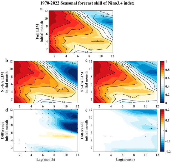
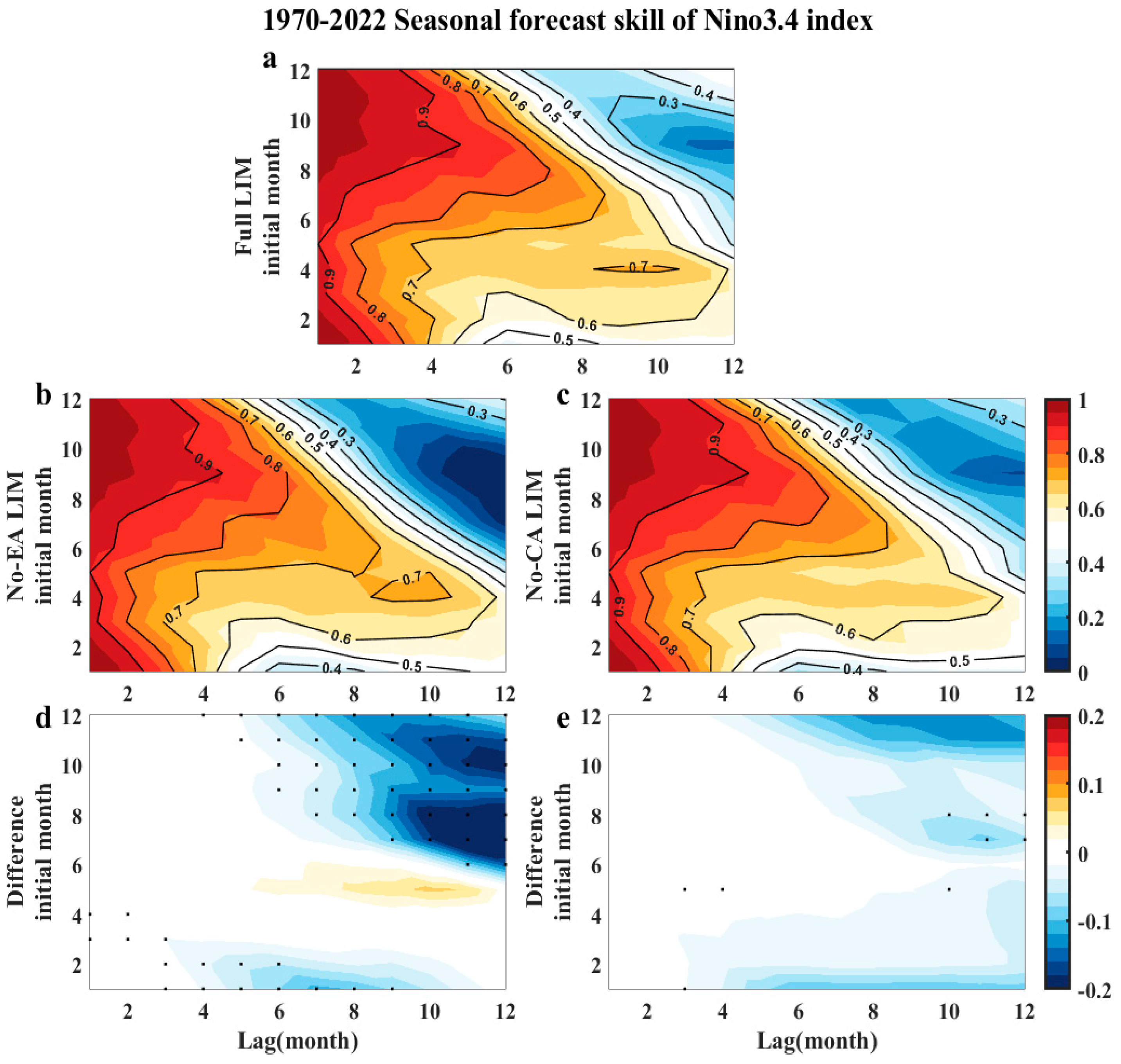
The EA mode plays a more important role in ENSO seasonal forecasts. Figure 1 shows the role of EA/CA modes in ENSO prediction (Figure 1). We evaluated the seasonal forecast skills for ENSO through the Autocorrelated Correlation Coefficient (ACC). In the Full LIM, the ACC is low when the initial month is in August to November at 9–12 months lead (Figure 1a), showing a distinct SPB feature. In the No-EA LIM, we decoupled the EA mode from the connections with the Tropical Pacific and CA mode (Figure 1b). To further explain the role of the EA mode in ENSO prediction, we compared the ACCs and calculated their difference between the Full LIM and the No-EA LIM. We found the ACC in the No-EA LIM is lower than that in Full LIM when the initial month is in June to December at a longer lead time (>8 months) (Figure 1d). This shows that the forecast skills will be reduced in the following spring and summer when the EA mode occurs. A decrease in the ACC skill in the No-EA LIM from November in the following summer is also confirmed (red line in Figure S5a). Compared to the EA mode, the decoupling of the CA mode does not significantly reduce the forecast skill for ENSO (Figure 1c, Figure 1e vs. Figure 1d). The forecast skill of the Niño3.4 index in the No-EA LIM (blue line in Figure S6) drops more rapidly than that in the No-CA LIM (red line in Figure S6). Meanwhile, the difference in forecast skills between the EA LIM and the Full LIM (blue line in Figure S7) is also larger than that between the CA LIM and the Full LIM (red line in Figure S7). In short, the EA mode plays a more important role than the CA mode in ENSO prediction.

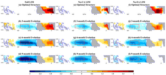
To explore the reasons why the Tropical Atlantic plays an important role in ENSO prediction, we employed an analysis of the evolution of the optimum initial conditions. Before analyzing the evolution, we calculated the ‘Maximum Amplification’ (MA) curve to analyze SSTA growth in the Niño3.4 area (Figure S8). The MA curve indicates that the growth in the Full LIM is peaked at a lag of 6 months. Thus, $\mathrm{\tau }$ = 6 months was chosen to examine the optimal initial conditions in the Tropical Atlantic. This method has recently been used for simulating the evolution of SSTAs in the Extratropical Pacific and other regions [19,20]. Then, we calculated the basic equation (Equation (1)) for the EA/CA Niño initial conditions (with no signal in the Tropical Pacific) to observe how these initial conditions evolve. After 3 months of evolution, a weak cold signal appears in the Tropical Pacific (Figure 2b). The cold signal is then strengthened through the local oceanic dynamics in the Tropical Pacific (Figure 2c) and eventually evolves into a mature ENSO event after 9 months (Figure 2d), while the warm signal in the Equatorial Atlantic is gradually weakened. This indicates that only Tropical Atlantic perturbations of SSTAs can trigger Tropical Pacific SSTAs without an original signal in the Tropical Pacific.

To further confirm the independent influence of the EA mode and CA mode on SSTA growth in the Niño3.4 area, we compared the Tropical Atlantic initial conditions and their evolutions with the No-CA LIM (Figure 2e–h) and the No-EA LIM (Figure 2i–l). The Tropical Atlantic optimal initial conditions in the No-CA LIM and No-EA LIM (Figure 2e,i) show strong warm SSTAs located in the Eastern and Central Equatorial Atlantic, which resemble the SSTAs spatial patterns of EA Niño and CA Niño, respectively [46]. Note that the local oceanic dynamics of the Equatorial Pacific were removed in the optimal structures (Figure 2a,e,i). Then, the cool signal appears in the Equatorial Pacific and finally evolves into a mature ENSO. This indicates that only oceanic perturbations in the Tropical Atlantic SST can trigger SSTAs in the Tropical Pacific. This phenomenon is also supported by the fact that the Atlantic Niño triggers La Niña [33,34,38].

The EA Niño and CA Niño have different impacts on ENSO development. In the No-CA LIM, there is an EA-like pattern in the Tropical Atlantic, showing a warm signal along the Western African coast (Figure 2e). After 3 months’ development, a weak cold signal appears in the Eastern Tropical Pacific due to the remote influence from the EA mode in the Tropical Atlantic (Figure 2f). Up until 6 months’ evolution, the cold signals develop into an ENSO-like pattern (Figure 2g). Finally, the cold SSTA peaks after 9 months of evolution and the warm SSTA in the Tropical Atlantic disappears (Figure 2h). This suggests that the EA mode plays an important role in ENSO development. In the No-EA LIM, the emergence of a CA-like pattern in the Tropical Atlantic shows, with a warm signal in the Central Tropical Atlantic (Figure 2i). Its evolution is similar to that in the No-CA LIM, but the cold signals caused by the CA mode are weaker than those caused by the EA mode (Figure 2j–l vs. Figure 2f–h), indicating that the CA mode is less important for triggering ENSO.

With the evolutions of the Tropical Pacific SSTAs, we find that the EA mode triggers a strong ENSO event and the CA mode leads to a moderate ENSO event (Figure 2g,h,k,l). Although the two modes both contribute to ENSO, the influence of the EA mode on ENSO development is stronger than that of the CA mode. This is consistent with our results that the influence of the CA Niño on ENSO prediction is relatively less than that of the EA Niño (Figure 1e vs. Figure 1d).

3.2. The Role of the EA/CA Mode in ENSO Diversity Predictability

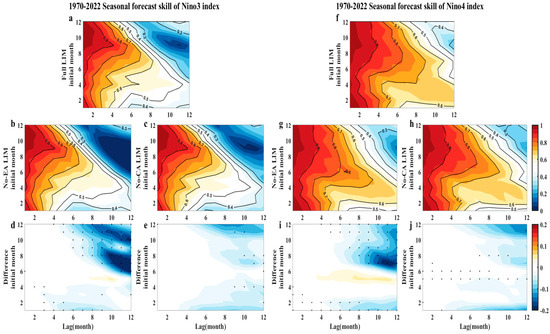
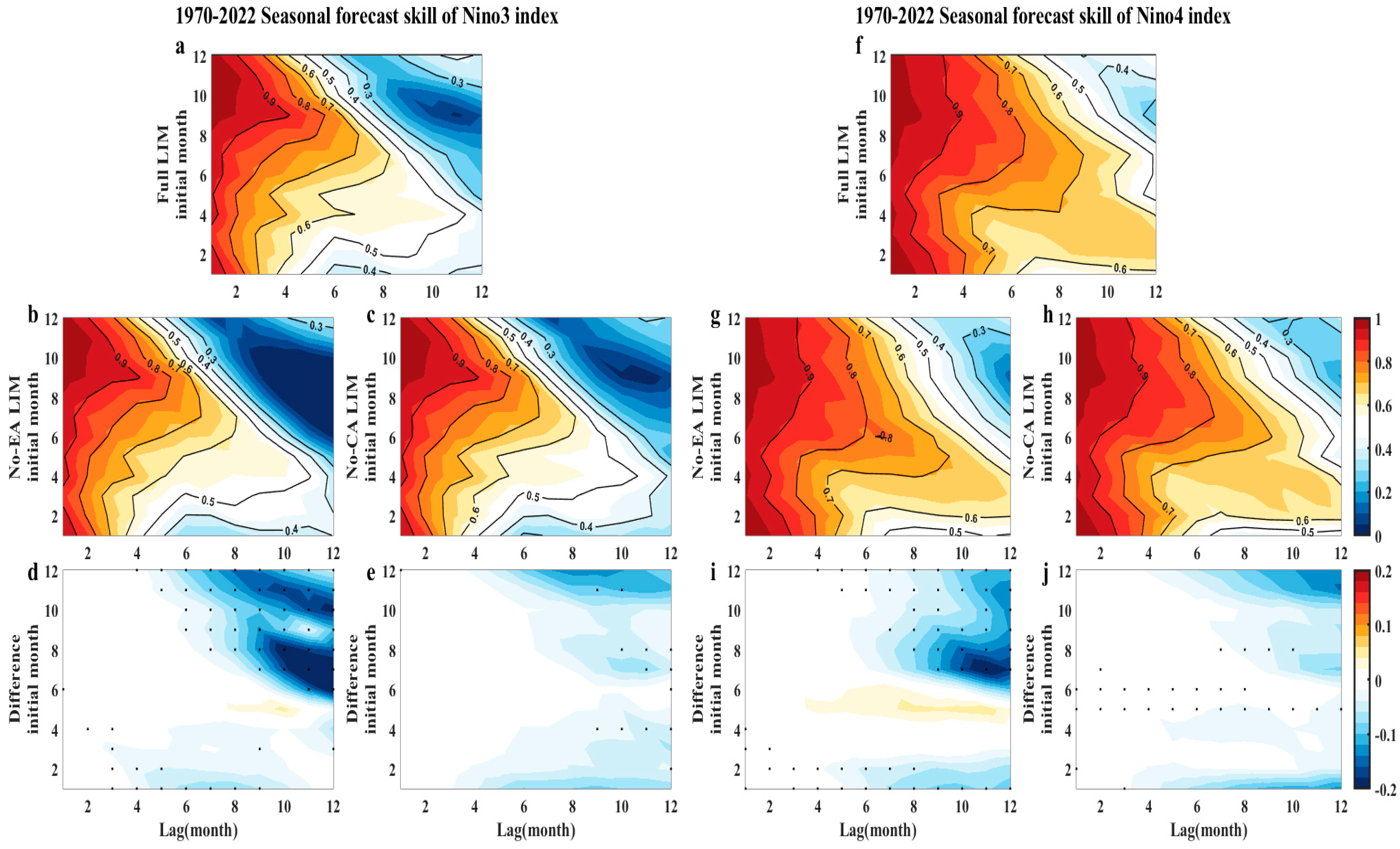
In the seasonal forecast skill of EP-ENSO (Niño3 index), the EA mode plays a more important role, especially in crossing EP-ENSO SPB. The No-EA LIM shows a weak forecast skill at 8–12 months lead, when the initial month is in June to December, compared to the Full LIM (Figure 3b vs. Figure 3a). For example, the ACCs are significantly weakened when the initial month is in August at a long lead time (>8 months), and the ACCs reduce from around 0.3 to 0. The ACC difference between the Full LIM and the No-EA LIM further indicates that the EA mode holds a significant position in the EP-ENSO prediction (Figure 3d). In contrast, the No-CA LIM’s ACCs do not show significant differences compared with the Full LIM (Figure 3c vs. Figure 3a), indicating that the CA mode has a less significance in EP-ENSO prediction. This conclusion is also supported by the differences (Figure 3d vs. Figure 3e, Figure S7b) and by the forecast skills from November (red and yellow lines in Figure S5b). These results indicate that the EA mode may play a more important role than the CA mode in seasonal forecast EP-ENSO predictability.

Similarly, a significant effect of the EA mode on CP-ENSO predictability can also be found. The smaller ACCs in the No-EA LIM are shown at 8–12 months lead, when the initial month is in June to October, compared to the Full LIM (Figure 3g vs. Figure 3f), and their differences also show a similar conclusion (Figure 3i). For example, the ACCs decrease from 0.6 to 0.4 when the initial month is in July, at long lead time (around 11 months). The changes in the ACCs in the No-CA LIM are not significant compared to the Full LIM (Figure 3h vs. Figure 3f, Figure 3j), suggesting that the CA mode has less of an effect on CP-ENSO predictability. This conclusion is also supported by the forecast skills from November (red and yellow lines in Figure S5c) and the differences in the forecast skills of Niño4 between the No-CA LIM as well as the No-EA LIM and the Full LIM (Figure S7c).

Overall, the EA mode plays a leading role in EP/CP-ENSO prediction when the initial month is in boreal summer to winter (June to December), and the effect of the CA mode on EP/CP-ENSO predictability is weak.

3.3. The Interdecadal Role of EA and CA Niño in ENSO Prediction

Recent studies have shown a much-weakened amplitude of the Atlantic Niño itself, but its remote impact on ENSO has remained strong and steady since the 1970s [49,50]. More specifically, the EA Niño has weakened significantly while the CA Niño has strengthened gradually since the 2000s [46]. Thus, it is necessary to discuss the interdecadal role of the EA and CA Niño on ENSO predictability before and after the 2000s.

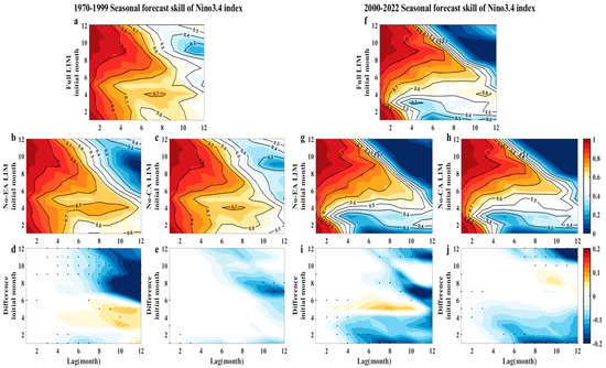
We evaluated the seasonal correlation forecast skill of the EA/CA mode in ENSO prediction before and after the 2000s (Figure 4). For the period of 1970–1999, the EA mode can significantly weaken the ENSO predictability. Through decoupling the EA mode in the No-EA LIM, the ACCs in the No-EA LIM are reduced significantly compared to the Full LIM at 8–12 months lead when the initial month is in boreal summer to winter (June to December) (Figure 4b vs. Figure 4a), resulting in a strong predictability barrier in the No-EA LIM (Figure 4d). The influence of the CA mode on ENSO predictability is not as strong as that of the EA mode before the 2000s. In the No-CA LIM, the ACC shows similar features compared with the Full LIM (Figure 4c vs. Figure 4a, Figure 4e). These results suggest that the SPB weakens significantly when the initial month is in the boreal summer and autumn by including the information of the EA mode, and SPB does not change significantly by including the information of the CA mode before 2000s. The changes in the forecast skills predicted from November before the 2000s also confirm this conclusion (Figure S9a).

For the period of 2000–2022, the effect of the EA mode on ENSO predictability was weakened. In the No-EA LIM, the ACCs declined from 0.2 to 0 during the boreal summer and winter (June to August and November to January), and the ACCs did not change compared to the Full LIM when the initial month was in boreal autumn (September to November) over long time scales (>6 months) (Figure 4g vs. Figure 4f). In the No-CA LIM, the ACCs decreased from 0.2 to 0 when the initial month was in boreal winter (November to January) at long lead times (>6 months) (Figure 4h vs. Figure 4f). By comparing the seasonal differences in ACCs before and after the 2000s (Figure 4i vs. Figure 4d and Figure 4j vs. Figure 4e), we found that the ENSO forecast skill in the No-CA LIM declined rapidly during winter after the 2000s. These results indicate that the influence of the EA mode on ENSO prediction has been weakened and the impact of the CA mode has been strengthened since the 2000s.

4. Discussion

In this paper, we found that the EA mode dynamics play a more important role than the CA mode in predicting ENSO over longer timescales (>6 months). The optimal initial structures also support this finding. The significant role of the EA mode in EP-ENSO and CP-ENSO is confirmed, while the CA mode has less of an effect on EP/CP-ENSO prediction. However, the influence of the EA mode on ENSO predictability has decreased, while the effect of CA mode has increased, since the 2000s. We prefer to consider that the most impact of the EA on ENSO prediction is from the period before the 2000s, and we would not deny the role of the CA, despite the fact that the influences of the EA mode are shown to be strong and those of the CA mode are shown to be weak in the results.

Recently, through Atmospheric model experiments, it has been demonstrated that the CA Niño has become an important factor influencing the climate conditions in regions surrounding the Tropical Atlantic [46]. Meanwhile, we confirm that the CA Niño has played an important role in crossing ENSO SPB during the winter after the 2000s. This conclusion also supports the point that the CA Niño’s remote impact on ENSO remains strong, despite the fact that the Atlantic Niño has weakened in recent decades. It is necessary to explore the CA mode in dynamical models to further improve ENSO predictions.

References

- Alexander, M.A.; Blade, I.; Newman, M.; Lanzante, J.R.; Lau, N.; Scott, J.D. The Atmospheric Bridge: The Influence of ENSO Teleconnections on Air—Sea Interaction over the Global Oceans. J. Clim. 2002, 15, 2205–2231. [Google Scholar] [CrossRef]
- Di Lorenzo, E.; Cobb, K.M.; Furtado, J.C.; Schneider, N.; Anderson, B.T.; Bracco, A.; Alexander, M.A.; Vimont, D.J. Central Pacific El Nino and decadal climate change in the North Pacific Ocean. Nat. Geosci. 2010, 3, 762–765. [Google Scholar] [CrossRef]
- Liu, Z.; Di Lorenzo, E. Mechanisms and Predictability of Pacific Decadal Variability. Curr. Clim. Chang. Rep. 2018, 4, 128–144. [Google Scholar] [CrossRef]
- Cai, W.; Wu, L.; Lengaigne, M.; Li, T.; McGregor, S.; Kug, J.; Yu, J.; Stuecker, M.F.; Santoso, A.; Li, X.; et al. Pantropical climate interactions. Science 2019, 363, eaav4236. [Google Scholar] [CrossRef] [PubMed]
- Capotondi, A.; Deser, C.; Phillips, A.S.; Okumura, Y.; Larson, S.M. ENSO and Pacific Decadal Variability in the Community Earth System Model Version 2. J. Adv. Model. Earth Syst. 2020, 12, e2019MS002022. [Google Scholar] [CrossRef]
- Kane, R.P. Extremes of the ENSO phenomenon and Indian summer monsoon rainfall. Int. J. Climatol. 1998, 18, 775–791. [Google Scholar] [CrossRef]
- Kripallani, R.H.; Kulkarni, A. Rainfall variability over South-east Asia—Connections with Indian monsoon and ENSO extremes: New perspectives. Int. J. Climatol. 1998, 17, 1155–1168. [Google Scholar] [CrossRef]
- Dutta, U.; Hazra, A.; Chaudhari, H.S.; Saha, S.K.; Pokhrel, S.; Verma, U. Unraveling the Global Teleconnections of Indian Summer Monsoon Clouds: Expedition from CMIP5 to CMIP6. Glob. Planet. Chang. 2022, 215, 103873. [Google Scholar] [CrossRef]
- Capotondi, A.; Sardeshmukh, P.D. Optimal precursors of different types of ENSO events. Geophys. Res. Lett. 2015, 42, 9952–9960. [Google Scholar] [CrossRef]
- Capotondi, A.; Ricciardulli, L. The influence of pacific winds on ENSO diversity. Sci. Rep. 2021, 11, 18672. [Google Scholar] [CrossRef] [PubMed]
- Tseng, Y.H.; Huang, J.H.; Chen, H.C. Improving the Predictability of Two Types of ENSO by the Characteristics of Extratropical Precursors. Geophys. Res. Lett. 2022, 49, e2021GL097190. [Google Scholar] [CrossRef]
- Chen, H.; Jin, Y.; Liu, Z.; Sun, D.; Chen, X.; McPhaden, M.J.; Capotondi, A.; Lin, X. Central-Pacific El Niño-Southern Oscillation less predictable under greenhouse warming. Nat. Commun. 2024, 15, 4370. [Google Scholar] [CrossRef]
- Jin, F. An Equatorial Ocean Recharge Paradigm for ENSO. Part I: Conceptual Model. J. Atmos. Sci. 1997, 54, 811–829. [Google Scholar] [CrossRef]
- Jin, F. An Equatorial Ocean Recharge Paradigm for ENSO. Part II: A Stripped-Down Coupled Model. J. Atmos. Sci. 1997, 54, 830–847. [Google Scholar] [CrossRef]
- Meinen, C.S.; McPhaden, M.J. Observations of Warm Water Volume Changes in the Equatorial Pacific and Their Relationship to El Niño and La Niña. J. Clim. 2000, 13, 3551–3559. [Google Scholar] [CrossRef]
- Vecchi, G.A.; Harrison, D.E. Tropical Pacific Sea Surface Temperature Anomalies, El Niño, and Equatorial Westerly Wind Events. J. Clim. 2000, 13, 1814–1830. [Google Scholar] [CrossRef]
- McPhaden, M.J. Evolution of the 2002/03 El Niño. Bull. Am. Meteorol. Soc. 2004, 85, 677–696. [Google Scholar] [CrossRef]
- Capotondi, A.; Sardeshmukh, P.D.; Ricciardulli, L. The Nature of the Stochastic Wind Forcing of ENSO. J. Clim. 2018, 31, 8081–8099. [Google Scholar] [CrossRef]
- Zhao, Y.; Jin, Y.; Li, J.; Capotondi, A. The Role of Extratropical Pacific in Crossing ENSO Spring Predictability Barrier. Geophys. Res. Lett. 2022, 49, e2022GL099488. [Google Scholar] [CrossRef]
- Zhao, Y.; Jin, Y.; Capotondi, A.; Li, J.; Sun, D. The Role of Tropical Atlantic in ENSO Predictability Barrier. Geophys. Res. Lett. 2023, 50, e2022GL101853. [Google Scholar] [CrossRef]
- Jin, Y.; Meng, X.; Zhang, L.; Zhao, Y.; Cai, W.; Wu, L. The Indian Ocean Weakens the ENSO Spring Predictability Barrier: Role of the Indian Ocean Basin and Dipole Modes. J. Clim. 2023, 36, 8331–8345. [Google Scholar] [CrossRef]
- Tang, Y.; Zhang, R.; Liu, T.; Duan, W.; Yang, D.; Zheng, F.; Ren, H.; Lian, T.; Gao, C.; Chen, D.; et al. Progress in ENSO prediction and predictability study. Natl. Sci. Rev. 2018, 5, 826–839. [Google Scholar] [CrossRef]
- Liu, Z.; Jin, Y.; Rong, X. Theory for the Seasonal Predictability Barrier: Threshold, Timing, and Intensity. J. Clim. 2019, 32, 423–443. [Google Scholar] [CrossRef]
- Jin, Y.; Lu, Z.; Liu, Z. Controls of Spring Persistence Barrier Strength in Different ENSO Regimes and Implications for 21st Century Changes. Geophys. Res. Lett. 2020, 47, e2020GL088010. [Google Scholar] [CrossRef]
- Webster, P.J.; Yang, S. Monsoon and Enso: Selectively Interactive Systems. Q. J. R. Meteorol. Soc. 1992, 118, 877–926. [Google Scholar] [CrossRef]
- Xue, Y.; Cane, M.A.; Zebiak, S.E.; Blumenthal, M.B. On the prediction of ENSO: A study with a low- order Markov model. Tellus Ser. A-Dyn. Meteorol. Oceanol. 1994, 46, 512–528. [Google Scholar] [CrossRef]
- Jin, E.K.; Kinter, J.L.; Wang, B.; Park, C.K.; Kang, I.S.; Kirtman, B.P.; Kug, J.S.; Kumar, A.; Luo, J.J.; Schemm, J.; et al. Current status of ENSO prediction skill in coupled ocean–atmosphere models. Clim. Dyn. 2008, 31, 647–664. [Google Scholar] [CrossRef]
- Jin, Y.; Liu, Z.; Lu, Z.; He, C. Seasonal Cycle of Background in the Tropical Pacific as a Cause of ENSO Spring Persistence Barrier. Geophys. Res. Lett. 2019, 46, 13371–13378. [Google Scholar] [CrossRef]
- Wu, R.; Kirtman, B.P.; van den Dool, H. An Analysis of ENSO Prediction Skill in the CFS Retrospective Forecasts. J. Clim. 2009, 22, 1801–1818. [Google Scholar] [CrossRef]
- Hou, M.; Duan, W.; Zhi, X. Season-dependent predictability barrier for two types of El Niño revealed by an approach to data analysis for predictability. Clim. Dyn. 2019, 53, 5561–5581. [Google Scholar] [CrossRef]
- Keenlyside, N.S.; Latif, M. Understanding Equatorial Atlantic Interannual Variability. J. Clim. 2007, 20, 131–142. [Google Scholar] [CrossRef]
- Polo, I.; Rodríguez-Fonseca, B.; Losada, T.; García-Serrano, J. Tropical Atlantic Variability Modes (1979–2002). Part I: Time-Evolving SST Modes Related to West African Rainfall. J. Clim. 2008, 21, 6457–6475. [Google Scholar] [CrossRef]
- Polo, I.; Martin-Rey, M.; Rodriguez-Fonseca, B.; Kucharski, F.; Mechoso, C.R. Processes in the Pacific La Niña onset triggered by the Atlantic Niño. Clim. Dyn. 2015, 44, 115–131. [Google Scholar] [CrossRef]
- Rodríguez Fonseca, B.; Polo, I.; García Serrano, J.; Losada, T.; Mohino, E.; Mechoso, C.R.; Kucharski, F. Are Atlantic Niños enhancing Pacific ENSO events in recent decades? Geophys. Res. Lett. 2009, 36, L20705. [Google Scholar] [CrossRef]
- Ding, H.; Keenlyside, N.S.; Latif, M. Impact of the Equatorial Atlantic on the El Niño Southern Oscillation. Clim. Dyn. 2012, 38, 1965–1972. [Google Scholar] [CrossRef]
- Martín-Rey, M.; Polo, I.; Rodriguez-Fonseca, B.; Kucharski, F. Changes in the interannual variability of the tropical Pacific as a response to an equatorial Atlantic forcing. Sci. Mar. 2012, 76, 105–116. [Google Scholar] [CrossRef]
- Martín-Rey, M.; Rodríguez-Fonseca, B.; Polo, I.; Kucharski, F. On the Atlantic–Pacific Niños connection: A multidecadal modulated mode. Clim. Dyn. 2014, 43, 3163–3178. [Google Scholar] [CrossRef]
- Ham, Y.G.; Kug, J.S.; Park, J.Y. Two distinct roles of Atlantic SSTs in ENSO variability: North Tropical Atlantic SST and Atlantic Niño. Geophys. Res. Lett. 2013, 40, 4012–4017. [Google Scholar] [CrossRef]
- Keenlyside, N.S.; Ding, H.; Latif, M. Potential of equatorial Atlantic variability to enhance El Niño prediction. Geophys. Res. Lett. 2013, 40, 2278–2283. [Google Scholar] [CrossRef]
- Wang, L.; Yu, J.Y.; Paek, H. Enhanced biennial variability in the Pacific due to Atlantic capacitor effect. Nat. Commun. 2017, 8, 14887. [Google Scholar] [CrossRef] [PubMed]
- Jiang, L.; Li, T. Impacts of Tropical North Atlantic and Equatorial Atlantic SST Anomalies on ENSO. J. Clim. 2021, 34, 1–58. [Google Scholar] [CrossRef]
- Ham, Y.; Kug, J.; Park, J.; Jin, F. Sea surface temperature in the north tropical Atlantic as a trigger for El Nino/Southern Oscillation events. Nat. Geosci. 2013, 6, 112–116. [Google Scholar] [CrossRef]
- Chang, P.; Fang, Y.; Saravanan, R.; Ji, L.; Seidel, H. The cause of the fragile relationship between the Pacific El Niño and the Atlantic Niño. Nature 2006, 443, 324–328. [Google Scholar] [CrossRef]
- Lübbecke, J.F.; McPhaden, M.J. On the Inconsistent Relationship between Pacific and Atlantic Niños. J. Clim. 2012, 25, 4294–4303. [Google Scholar] [CrossRef]
- Tokinaga, H.; Richter, I.; Kosaka, Y. ENSO Influence on the Atlantic Niño, Revisited: Multi-Year versus Single-Year ENSO Events. J. Clim. 2019, 32, 4585–4600. [Google Scholar] [CrossRef]
- Zhang, L.; Wang, C.; Han, W.; McPhaden, M.J.; Hu, A.; Xing, W. Emergence of the Central Atlantic Niño. Sci. Adv. 2023, 9, eadi5507. [Google Scholar] [CrossRef]
- Tokinaga, H.; Xie, S. Weakening of the equatorial Atlantic cold tongue over the past six decades. Nat. Geosci. 2011, 4, 222–226. [Google Scholar] [CrossRef]
- Prigent, A.; Lübbecke, J.F.; Bayr, T.; Latif, M.; Wengel, C. Weakened SST variability in the tropical Atlantic Ocean since 2000. Clim. Dyn. 2020, 54, 2731–2744. [Google Scholar] [CrossRef]
- Losada, T.; Rodríguez-Fonseca, B. Tropical atmospheric response to decadal changes in the Atlantic Equatorial Mode. Clim. Dyn. 2016, 47, 1211–1224. [Google Scholar] [CrossRef]
- Lübbecke, J.F.; Rodríguez Fonseca, B.; Richter, I.; Martín Rey, M.; Losada, T.; Polo, I.; Keenlyside, N.S. Equatorial Atlantic variability—Modes, mechanisms, and global teleconnections. Wires Clim. Chang. 2018, 9, e527. [Google Scholar] [CrossRef]
- Penland, C.; Matrosova, L. A Balance Condition for Stochastic Numerical Models with Application to the El Niño-Southern Oscillation. J. Clim. 1994, 7, 1352–1372. [Google Scholar] [CrossRef]
- Penland, C.; Sardeshmukh, P.D. The Optimal Growth of Tropical Sea Surface Temperature Anomalies. J. Clim. 1995, 8, 1999–2024. [Google Scholar] [CrossRef]
- Newman, M.; Alexander, M.A.; Scott, J.D. An empirical model of tropical ocean dynamics. Clim. Dyn. 2011, 37, 1823–1841. [Google Scholar] [CrossRef]
- Newman, M.; Sardeshmukh, P.D. Are we near the predictability limit of tropical Indo-Pacific sea surface temperatures? Geophys. Res. Lett. 2017, 44, 8520–8529. [Google Scholar] [CrossRef]
- Rayner, N.A.; Parker, D.E.; Horton, E.B.; Folland, C.K.; Alexander, L.V.; Rowell, D.P.; Kent, E.C.; Kaplan, A. Global analyses of sea surface temperature, sea ice, and night marine air temperature since the late nineteenth century. J. Geophys. Res. Atmos. 2003, 108, 4407. [Google Scholar] [CrossRef]
- Deser, C.; Phillips, A.S.; Alexander, M.A. Twentieth century tropical sea surface temperature trends revisited. Geophys. Res. Lett. 2010, 37, 10. [Google Scholar] [CrossRef]
- Kug, J.; Jin, F.; An, S. Two Types of El Niño Events: Cold Tongue El Niño and Warm Pool El Niño. J. Clim. 2009, 22, 1499–1515. [Google Scholar] [CrossRef]
- Hasselmann, K. Stochastic climate models Part I. Theory. Tellus 1976, 28, 473–485. [Google Scholar]
- Takahashi, K.; Montecinos, A.; Goubanova, K.; Dewitte, B. ENSO regimes: Reinterpreting the canonical and Modoki El Niño: Reinterpreting Enso Modes. Geophys. Res. Lett. 2011, 38, L10704. [Google Scholar] [CrossRef]
- Vimont, D.J.; Alexander, M.A.; Newman, M. Optimal growth of Central and East Pacific ENSO events. Geophys. Res. Lett. 2014, 41, 4027–4034. [Google Scholar] [CrossRef]
- Zhang, L.; Han, W. Barrier for the Eastward Propagation of Madden-Julian Oscillation Over the Maritime Continent: A Possible New Mechanism. Geophys. Res. Lett. 2020, 47, 2020GL090211. [Google Scholar] [CrossRef]
- Steiger, J.H. Tests for comparing elements of a correlation matrix. Psychol. Bull. 1980, 87, 245–251. [Google Scholar] [CrossRef]
Disclaimer/Publisher’s Note: The statements, opinions and data contained in all publications are solely those of the individual author(s) and contributor(s) and not of MDPI and/or the editor(s). MDPI and/or the editor(s) disclaim responsibility for any injury to people or property resulting from any ideas, methods, instructions or products referred to in the content. |
© 2024 by the authors. Licensee MDPI, Basel, Switzerland. This article is an open access article distributed under the terms and conditions of the Creative Commons Attribution (CC BY) license (https://creativecommons.org/licenses/by/4.0/).