Abstract
Obtaining precise seasonal yield estimates is challenging, with weather forecast accuracy being a key factor. This study examines the impact of different weather data forecasting methods on yield estimation. Initially, we evaluated the suitability of the WOFOST model for highland barley (HB) and wheat on the northeastern Tibetan Plateau. Yield forecasts were conducted using nine historical weather selection methods under two scenarios, differing in their use of 10-day TIGGE data. The results showed that different weather data fusion methods led to varying forecasted yields. For HB, sequential selection and an improved KNN algorithm were optimal, while for wheat, sequential selection performed best. Early-season forecasts had lower accuracy, while predictions after flowering were more reliable. Incorporating TIGGE short-term forecasts into historical weather data improved HB yield forecasts, with 98.2% of days having an average relative error (ARE) below 20%. For wheat, using only historical weather data provided more stable yield forecasts, with 93.1% of days having an ARE below 20%. The weather data fusion strategy for yield forecasts offered reliable prediction accuracy without the need for full-cycle weather observation.
1. Introduction
The need for early and reliable crop yield forecasting is rising among farmers and decision-makers [1,2,3]. Crop yield forecasting is crucial for supporting government agricultural decision-making and aiding farmers in agricultural management practices to enhance farm planning, fertilizer management, crop insurance, and marketing [3,4].
Early crop yield forecasting has primarily mainly relied on two methods: statistical regression-based models and dynamic process-based crop models. Statistical regression–based models generate forecasts through regression equations derived from statistical relationships between crop yields and related factors, such as meteorological factors and/or vegetation indices from remote sensing data [3,5]. These models encompass both linear and non-linear regression approaches. Previous studies have shown that relatively simple equations using two or three variables can explain more than two-thirds of observed yield variations for most crops [6]. However, linear regression models typically perform poorly compared to nonlinear regression models due to the nonlinear relationships among crop yields, environmental factors, and management practices [7,8,9]. For example, in a maize yield simulation study conducted in the United States, a random forest model demonstrated higher simulation accuracy than linear regression [10]. Additionally, in a study that forecasted corn and soybean yields on a county-by-county basis in the “corn belt” area of the Midwestern and Great Plains regions of the United States, an artificial neural network (ANN) outperformed multivariate linear regression (MLR) models [8]. While statistical regression-based models have shown promise in crop yield forecasting [8], their accuracy is constrained by the availability and quantity of statistical data. Furthermore, these models lack mechanistic understanding, limiting their ability to elucidate the underlying processes and relationships between crop production and climatic variables. Crop models that overcome these limitations are useful tools in this regard. Process-based crop models adeptly describe key physical and physiological processes by capturing the intricate interactions among crops, soils, weather, and management practices [11,12]. Crop models have been widely used to explore the impacts of genotype, environment, and management on crop production, guiding sound crop management practices and informed decision-making [13]. Therefore, we employ a crop simulation model for crop yield forecasting in this study.
However, using crop models for forecasting yields introduces the challenge of unknown weather conditions between the last observed day and the maturity date, which can lead to significant uncertainty in the forecasted yield [1]. Previous studies have attempted to address this challenge by substituting unknown future weather data with average values of historical data for forecasting seasonal yields [14]. However, these simulations proved less accurate in the early stages of the growing season due to the nonlinear relationship between crop growth and climate conditions [15]. The potential of using historical climate information for yield forecasting has been assessed, assuming past climate could reflect the range of variability of future climate [16]. The mean crop model output yield method, which combines up-to-date weather observations with historical climatology data to substitute the unknown weather data for the rest of the season, has demonstrated good or acceptable accuracy [2,17]. Therefore, this method is used in this study.
Despite this approach, addressing two challenging steps is necessary for its effective application. The first is selecting historical weather data that closely matches the current year’s climate conditions. The second is determining the forecast periods from emergence to maturity, which can be used to forecast crop yields that best match the observed yields. To tackle these challenges, we divided the growth period into distinct stages based on observed phenological data and tested three weather data fusion methods: sequential historical weather selection from preceding years, a KNN-based analogue weather selection, and an improved KNN-based analogue weather selection to choose historical weather data for each forecast period. By identifying the optimal forecast period based on the most effective method, we tested two hypotheses. The first hypothesis is that different historical weather selection methods are needed for different forecast periods. The second hypothesis is that the accuracy of the crop yield forecast gradually improves, with more observed weather data becoming available as the forecast period progresses. Various types of seasonal forecasts have been utilized for crop yield forecasting, including General/Regional Circulation Models (GCM/RCM)-based forecasts, forecasts based on phases of the El Niño Southern Oscillation (ENSO) and Southern Oscillation Index (SOI), empirically derived forecasts, and forecasts based on analogue years [18,19,20,21,22,23]. Recently, researchers have focused on combining forecast and historical data to address unknown future weather data [5,24,25,26]. The question of whether using forecast data can enhance the accuracy of HB and wheat yield forecasting in Qinghai remains unanswered. To answer the question, we integrate THORPEX Interactive Grand Global Ensemble (TIGGE) short-term forecast data with historical weather data for crop yield forecasting. Additionally, we tested a third hypothesis: the incorporation of TIGGE short-term forecast data will significantly increase crop yield forecast accuracy.
This study focuses on Qinghai Province, an ecologically sensitive and underdeveloped region on the northeastern Tibetan Plateau characterized by a cold, dry plateau climate and single-season cereal cropping [27]. Yield forecasting is particularly crucial in this area. However, limited statistical data in this area hinders the usefulness of statistical regression models for yield forecasting. Hence, this study aims to utilize the WOFOST model, TIGGE short-term forecast data, and historical weather data to develop a more accurate yield forecasting method for wheat and HB in Qinghai Province. This study aims to (1) identify the most suitable weather data fusion methods for different growth periods of wheat and HB in Qinghai Province; (2) determine the optimal forecast period for yield forecasting; and (3) evaluate whether TIGGE forecast data can enhance yield forecasting accuracy.
2. Materials and Methods
2.1. Study Area
Agriculture is a fundamental industry in Qinghai province, located on the northeastern Tibetan Plateau (89°35′–103°04′ N and 31°36′–39°19′ E) (Figure 1). It is a critical foundation for socio-economic development in Qinghai and the livelihood of farmers and herdsmen [28]. The area is characterized by high elevations in the west and lower elevations in the east. Qinghai Province experiences a dry climate with low precipitation and long sunshine hours. Due to the terrain, climate, and temperature difference, agriculture in Qinghai province can only sow once a year [27]. Generally, the annual average temperature in Qinghai Province is higher in the north and lower in the south. Wheat and HB are the primary cereals cultivated in the province. In Qinghai Province, HB and wheat are typically sown from March to April and harvested in September. In regions above 4200m altitude, only HB can be cultivated due to its cold-resistant characteristics. Conducting seasonal yield predictions for HB and wheat at the field scale can significantly impact direct farm management practices and local economic considerations, such as sale prices, grain storage, and safety precautions.
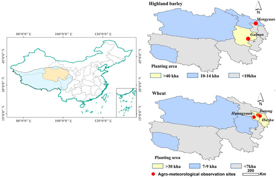
Figure 1.
Locations of the study area and agro-meteorological observation sites.
2.2. WOFOST Model
The WOFOST model, jointly developed by Wageningen Agricultural University and the Center for World Food Studies [29], is a comprehensive crop growth model that encompasses major processes such as phenological development, leaf development and light interception, CO2 assimilation, root growth, transpiration, respiration, assimilate partitioning, and dry matter formation [30]. The yield formation principles in the WOFOST model have undergone thorough validation for various crops, including wheat, maize, and rice [13]. To conduct WOFOST simulations, four inputs are needed: weather, soil, crop, and management. In the current version of WOFOST, yield-reducing factors such as weeds, pests, frost, and diseases are not taken into account. In our study, we primarily focus on the impact of weather data generation methods on yield forecast. Therefore, yield simulations were conducted under water-limited conditions, without accounting for the influence of soil fertility. For more detailed information on the WOFOST model, please visit the following link: https://www.wur.nl/en/Research-Results/Research-Institutes/Environmental-Research/Facilities-Tools/Software-models-and-databases/WOFOST.htm (accessed on 4 May 2025).
2.3. Datasets
2.3.1. Field Trials Data
As shown in Table 1, field trials of HB were carried out at two agro-meteorological observation stations situated in Guinan County and Menyuan Hui Autonomous County. These locations are major HB planting areas in the Hainan Tibetan Autonomous Prefecture and Haibei Tibetan Autonomous Prefecture, respectively. Field trials of wheat were conducted at three agro-meteorological observation stations located in Datong Hui and Tu Autonomous County, Huzhu Tu Autonomous County, and Huangyuan County. These locations are important wheat planting areas in Xining City, Haidong City, and Xining City, respectively. In total, these trials were conducted at five agro-meteorological observation stations in Qinghai Province (see Figure 1), all under the auspices of the Chinese Meteorological Administration (CMA). Soil information, crop varieties, and management data—phenological, observed data for field trials—were gathered from the agricultural meteorological station. Soil information included saturated water content, wilting coefficient, and field water holding capacity. Phenological, observed data covered key stages such as planting, emergence, three-leaf stage, tillering, jointing, boot, heading, anthesis, milk, and maturity dates.

Table 1.
Field trial information.
2.3.2. Weather Data
The weather data include historical weather data and TIGGE forecast data. The historical weather data were obtained from the Qinghai Meteorological Administration (http://qh.cma.gov.cn/ (accessed on 4 May 2025)), including daily sunshine hours, maximum air temperature, minimum air temperature, mean vapor pressure, mean windspeed at 2 m above the surface, and precipitation. Solar radiation was calculated with the Angstrom–Prescott model and sunshine hours [31]. TIGGE forecast data, with a spatial resolution of 0.5° × 0.5°, span from 2007 to 2019 and were obtained from the TIGGE dataset (https://apps.ecmwf.int/datasets/data/tigge/levtype=sfc/type=fc/ (accessed on 4 May 2025)). Established in 2008, TIGGE is a valuable resource for prediction studies, combining ensemble forecasts from up to ten global weather services utilizing diverse generation methods and resolutions. This dataset provides unique opportunities to enhance our understanding of the predictability of specific weather systems [32,33].
2.4. General Framework
Figure 2 illustrates the flowchart depicting the HB and wheat yield forecasting process involving the WOFOST model, TIGGE short-term forecast data, and historical weather data. The research methodology comprised four steps.
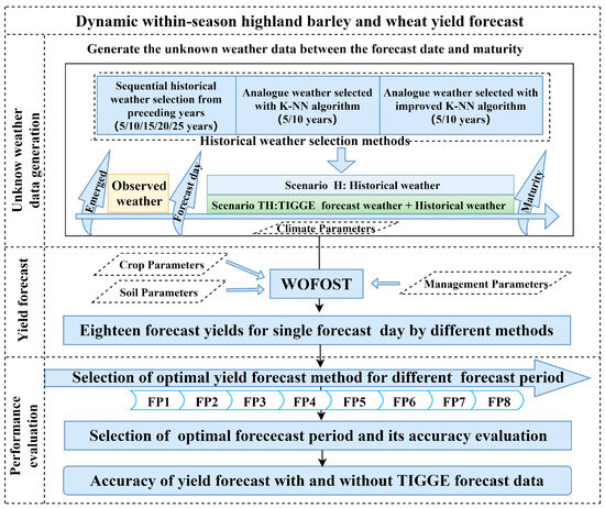
Figure 2.
Yield forecasting framework (note: FP 1–8 refer to the stages from emergence to three leaves, from three leaves to tillering, from tillering to jointing, from jointing to boot, from boot to heading, from heading to flowering, from flowering to milk, and from milk to maturity, respectively).
- Step 1: Dynamic yield forecasts with different methods
Yield forecast experiments were simulated for each field trial (Table 1). For each forecast year, daily yield forecasts were conducted from emergence to maturity. Observed weather data were used before the forecast date, while the unknown weather data for the rest of the growth period were generated using two methods. The first method used only historical weather data (Scenario H), and the other method combined TIGGE weather forecast data for 10 days post-forecast date with historical data (Scenario TH). Three methods were used to select historical data in two scenarios. The first method involved selecting historical weather data from leading years, specifically 5 (5y), 10 (10y), 15 (15y), 20 (20y), or 25 (25y) years prior to the forecast year. The second method utilized a k-nearest neighbor (KNN) algorithm based on Euclidean distance. The third method employed an improved KNN algorithm for selecting 5 (IKNN-5y) or 10 (IKNN-10y) similar historical years based on the Euclidean distance of weekly cumulative weather factors. The weather data combinations chosen by each method were used to drive the model for yield forecasting, and the mean yields obtained through simulation for each combination served as the final forecast. Simulations were conducted for each forecast year from emergence to maturity, considering the total number of days, the historical years selected for each method (105), and scenarios with or without forecast data (2).
- Step 2: Determination of optimal weather data fusion methods within different forecast periods
To assess forecast possibilities within distinct forecast periods, we analyzed optimal weather data fusion methods. Initially, we calculated root mean square error (RMSE) values for forecast yield within each forecast period: emergence to three leaves (FP 1), three leaves to tillering (FP 2), tillering to jointing (FP 3), jointing to boot (FP 4), boot to heading (FP 5), heading to flowering (FP 6), flowering to milk (FP 7), and milk to maturity (FP 8). Subsequently, we normalized evaluation indicators for each of the nine methods used in each experimental year to ensure consistent units of measure. This normalization was based on the difference in RMSE between the best simulation method and other methods for each forecast year. Finally, the mean of the normalized evaluation indicators for each of the nine methods was calculated for each experimental year (). Lower values of indicated higher accuracy.
- Step 3: Evaluation of optimal forecast period for yield forecasting
The maximum, minimum, mean, and coefficient of variation (CV) of the RMSE for all experimental years were calculated using the optimal weather data fusion methods across different forecast periods. The optimal forecast period for crop yield forecasting was determined based on the RMSE results. Additionally, the variation trend in the mean absolute relative error (ARE) for all crops across all experimental years in the optimal yield forecast periods was studied.
- Step 4: Evaluation of the effect of TIGGE forecast data on yield forecast
To assess whether TIGGE forecast data could enhance yield forecasting, we evaluated the yield forecasts for HB and wheat under scenarios H and TH. Initially, we calculated average ARE values for all forecast days within the optimal forecast periods for each crop under scenarios H and TH. We conducted a statistical analysis of the frequency of ARE values falling into six numerical intervals: 0–5%, 5–10%, 10–20%, 20–30%, 30–40%, and >40%. We then analyzed and compared the probability distribution characteristics of average ARE values for different crops under different scenarios. An increase in the number of average ARE values falling into the lower numerical intervals indicated higher overall accuracy in a given scenario, reflective of superior yield forecast performance. Finally, we comprehensively evaluated the influence of incorporating TIGGE forecast data on yield forecasts from multiple perspectives.
2.5. Statistical Analysis
To assess model performance and yield forecast accuracy, we employed several statistical indicators, including (1) RMSE (Equation (1)), which indicates the average magnitude of errors in a set of forecasts, with lower values denoting higher accuracy; (2) coefficient of determination (R2, Equation (2)), which measures how well the model fits the observed data, with values closer to 1 indicating a better fit; (3) ARE (Equation (3)), which indicates errors in the single-day forecast, with lower values indicating higher accuracy; and (4) Lin’s concordance correlation coefficient (LCCC, Equations (4) and (5)), which denotes the degree to which forecasted and observed values follow the 1:1 line through the origin, with values approaching 1 indicating greater accuracy [34]. Accurate model forecasts are indicated by lower RMSE and ARE values, higher R2 values, and LCCC values approaching 1 [3].
where S and O are the simulated and observed values of given variables; n is the total number of simulation times; and is the mean value of observed values. is the mean value of simulated values. and are the variances of observed and simulated values, respectively.
3. Results
3.1. Model Performance
Genetic parameters were calibrated and verified for three distinct HB cultivars and three different wheat cultivars. These parameters were then utilized to simulate anthesis dates, maturity dates, growth period from sowing to maturity, and grain yields. The simulations demonstrated robust predictions for both HB and wheat cultivars (Figure 3). The LCCC ranged from 0.66 to 0.76 for HB and 0.55 to 0.95 for wheat. In terms of phenology simulations, the RMSE ranged from 1.78 to 2.87 days for HB and 1.75 to 3.79 days for wheat. The R2 values ranged from 0.44 to 0.76. For grain yield simulations, the RMSE values were 292.65 kg/ha for HB and 362.85 kg/ha for wheat, with R2 values being 0.73 and 0.9, respectively. These results collectively indicate that the genetic parameters proved effective in predicting phenology and grain yield for both HB and wheat cultivars.
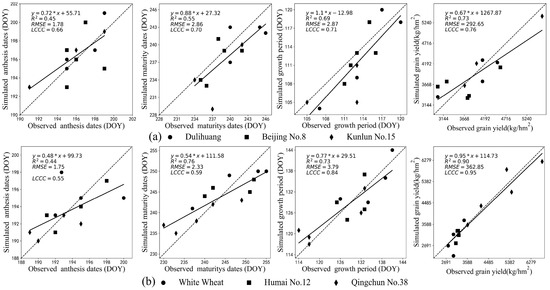
Figure 3.
Comparison of WOFOST-simulated and observed dates of anthesis and maturity, length of growth period, and grain yield for highland barley (a) and wheat (b) cultivars. Note: “*” indicates multiplication.
3.2. Determination of Optimal Weather Data Fusion Methods
We assessed the accuracy of yield forecasts for HB and wheat across eight forecast periods (FP1-FP8) using various weather data fusion methods (Figure 4). Different methods proved most suitable for distinct growth stages. Under scenario TH, the optimal methods for HB were 5y, 5y, IKNN10, IKNN10, IKNN10, IKNN5, IKNN5, and IKNN5 for FP1-FP8, respectively. Similarly, the optimal methods for wheat were 5y, 5y, 15y, 15y, 5y, 10y, 10y, and 5y for FP1-FP8, respectively. Under scenario H, the optimal methods for HB were 10y, 5y, 10y, 20y, 20y, KNN10, IKNN10, and 5y for FP1-FP8, respectively. For wheat, the optimal methods were 5y, 5y, 5y, 10y, 5y, 10y, 10y, and IKNN10y for FP1-FP8, respectively. Significant differences were observed among the nine weather data fusion methods used in FP1-FP6, but these differences were less pronounced in FP7 and FP8 than in FP1-FP6. Overall, sequential-based selection and improved KNN algorithm-based selection were more suitable for HB, with these two methods being optimal in 8 and 7 of 16 forecast periods, respectively. For wheat, sequential-based selection was more suitable, with this method being optimal in 15 out of the 16 forecast periods.
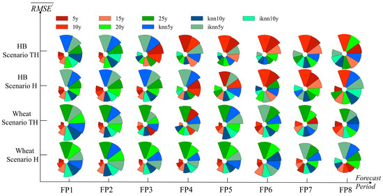
Figure 4.
Performance of different weather data fusion methods. (Note: the radius length of each pie chart section represents the value of , and the shorter the radius, the better the performance of the method. Scenarios TH and H refer to yield forecasts with and without TIGGE forecast data, respectively. FP 1–8, as explained in Figure 2. HB is highland barley).
3.3. Optimal Forecast Period for Yield Forecasting and Its Accuracy
RMSE values between observed and simulated yield were calculated for each forecast period to identify the optimal forecast period (Figure 5). The results showed that the minimum overall RMSE value was less than 145.1 kg/ha for both HB and wheat. Under scenario TH, the maximum and mean RMSE values for wheat increased and then decreased in later forecast periods, reaching their peak at FP5. For wheat under scenario H and for HB under scenarios H and TH, maximum and mean RMSE values exhibited an overall decreasing trend with increasing forecast periods. CV for both HB and wheat declined as growth stages progressed under both scenarios, indicating an increase in yield forecast accuracy with the development of the forecast period. Overall, optimal yield forecast periods were FP7 and FP8. Maximum RMSE values for these two periods were found to be 869.4 kg/ha and 589.52 kg/ha, respectively (scenario TH of HB), 1109.1 kg/ha and 588.99 kg/ha (Scenario H of HB), 1969.068 kg/ha and 791.47 kg/ha (Scenario TH of wheat), and 1230.6 kg/ha and 690.65 kg/ha (Scenario H of wheat). The corresponding CV values were 0.45 and 0.43, respectively (Scenario TH of HB), 0.65 and 0.5 (Scenario H of HB), 0.88 and 0.62 (Scenario TH of wheat), and 0.88 and 0.6 (Scenario H of wheat).
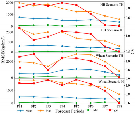
Figure 5.
RMSE values for optimal weather data fusion (note: scenarios TH and H refer to yield forecasts with and without TIGGE forecast data, respectively. FP 1–8, as explained in Figure 2).
Additional analysis focused on day-to-day accuracy changes within the optimal forecast periods using ARE performance (Figure 6). These periods ranged from flowering to maturity, including FP7 and FP8. For HB, upper quartile values ranged from 12.07% to 18.84% and 11.35% to 19.06%, with medians ranging from 9.14% to 13.71% and 6.77% to 12.6% under scenarios TH and H, respectively. For wheat, upper quartile values concentrated in the ranges of 8.06–41.22% and 5.95–10.44% under scenarios TH and H, respectively, with medians in ranges of 3.89–12.12% and 2.44–8.09%, respectively. The box lengths showed a decreasing trend for HB under both scenarios, similar to wheat under TH, indicating a more concentrated ARE distribution. Specifically, the box lengths for HB under scenario H and for wheat under scenario TH showed a significant decreasing trend. However, the box lengths for wheat under scenario TH exhibited considerable fluctuation without a clear trend. Overall, the yield forecast for HB performed better under scenario TH, while the yield forecasts for wheat performed better under scenario H. The best performance for both HB and wheat occurred in later growth stages under scenarios H and TH, respectively. Additionally, uncertainties in the yield forecasts for both HB and wheat under scenario TH declined as the forecast days approached maturity.
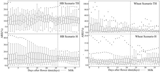
Figure 6.
Absolute relative error (ARE) values within the optimal forecast period. (Note: scenarios TH and H refer to yield forecasts with and without TIGGE forecast data, respectively. HB is highland barley).
3.4. Evaluation of Yield Forecast with and Without TIGGE Forecast Data
Yield forecasts for HB were evaluated with and without TIGGE forecast data (Figure 7). Under scenario TH, observed and forecasted HB yields had an average ARE mainly ranging from 10 to 20%, with a maximum of less than 30%. Approximately 93.2% of ARE values were less than 20%, but only 45.2% were less than 10%. Under scenario H, observed and forecasted HB yields mainly had average ARE values between 0 and 5% (26.8% of values), 5 and 10% (29.9% of values), and 10 and 20% (30.3% of values). Approximately 87% of ARE values were less than 20%, and 56.7% were less than 10%. However, 4.4% of ARE values were greater than 30%. The use of TIGGE forecast data had more stable but less accurate forecast potential for HB yield forecast compared with using only historical weather data. For wheat, there was a wider ARE distribution under both scenarios, and a higher proportion (37.9% under TH and 47.7% under H) of ARE values were below 5%. Yield forecast using TIGGE forecast data led to a higher proportion of accurate forecasts (greater than 20%), accounting for 22.7% under TH and 6.8% under H. Therefore, using only historical weather data provided more stable and reliable yield forecasts for wheat.
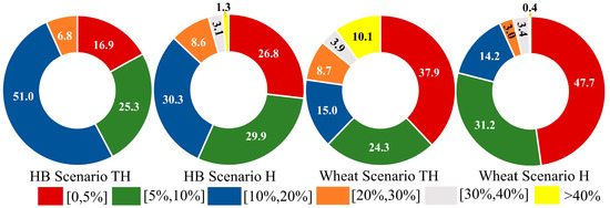
Figure 7.
Probability distributions of absolute relative error (ARE). (Note: Every pie chart section represents the probability proportion of the average ARE during the optimal forecast periods falling within different numerical intervals. Scenarios TH and H refer to yield forecast with and without TIGGE, respectively. HB is highland barley. Percentages are rounded to one decimal place; the total may not equal exactly 100%).
4. Discussion
4.1. Dynamic Yields Forecast with Different Weather Data Fusion Methods
The prevalence of miniature weather stations has facilitated the acquisition of meteorological data from crop emergence to any forecast date, emphasizing the prediction of unknown meteorological data between the forecast day and the maturity date using crop models [2]. Three historical year selection methods were employed: sequential historical year selection, KNN algorithm-based analogue selection, and improved KNN algorithm-based analogue selection. The sequential historical year selection method, based on the third law of geography [35], was divided into five periods (5y, 10y, 15y, 20y, and 25y prior to the experimental year) due to significant land use changes in Qinghai Province. The KNN algorithm-based analogue selection method has been applied to similar meteorological year selections for a long time [36,37]. The KNN algorithm-based analogue selection method and the improved KNN algorithm-based analogue selection methods used in this study were based on the Euclidean distance of single-day meteorological factors and the cumulative value of seven-day meteorological factors, respectively. These two methods provided greater flexibility in historical year selection compared to the sequential method. While a different study employed the vectorial angles method for historical year selection, considering the similarity between forecast and historical weather, this study focused on the similarity between the forecast day and historical weather to minimize potential errors arising from inaccurate weather forecasts [26].
4.2. Performance of Optimal Weather Data Fusion Methods for Different Forecast Periods
Various weather data fusion methods exert distinct impacts on yield forecast. Phenological data guided the division of forecast periods into eight periods, considering the different effects of meteorological factors on crop growth and development at each stage. Determining optimal forecast periods based on the number of days to maturity or after planting can be challenging due to maturity date uncertainties and variations in growth stages across different years. Thus, employing phenological information for practical start points of optimal forecast periods was deemed more pragmatic [2,3,5,21]. Under two scenarios, this study identified optimal weather data fusion methods, revealing that sequential-based selection and the improved KNN algorithm-based analogue selection were key for HB, while sequential-based selection dominated for wheat. Previous research has highlighted the effectiveness of the KNN algorithm-based analogue selection in predicting certain meteorological variables but noted its limitations in rainfall prediction, often attributed to the high uncertainty and non-uniform distribution of rainfall [38]. Similarly, this study found that the improved KNN algorithm-based analogue selection outperformed the traditional KNN algorithm-based method in forecasting corn yield on the Loess Plateau [2]. The observed differences could be linked to the sensitivity of rainfall simulation accuracy in arid or semi-arid regions where the study crops, including HB and wheat, are located. Moreover, this study noted significant differences among the nine weather data fusion methods during FP1-FP6, suggesting that the accuracy of yield forecasts was notably influenced by the number of observed data points in the simulated meteorological dataset. Therefore, selecting the optimal weather data fusion method during the early stages of a yield forecast was deemed crucial.
4.3. Performance of Optimal Forecast Period for Yield Forecasting
As the forecast period advanced, the precision of yield forecasts progressively improved, attributed to the diminishing uncertainty in the simulated meteorological data. Optimal accuracy for both HB and wheat yield forecasts was attained in forecast periods FP7 and FP8, initiating from the flowering stage. The average duration from flowering to maturity were 43 and 50 days for HB and wheat, respectively. Consistent with prior studies, crop models demonstrated reliable yield forecasts within the two weeks to two months leading up to maturity [5,39,40,41]. Analysis of the daily changes in ARE within the optimal forecast periods revealed superior performance for HB yield forecasts under scenario TH, while wheat yield forecasts excelled under scenario H. Furthermore, forecasts for HB under scenario H and wheat under scenario TH exhibited enhanced performance in the later stages of the optimal forecast periods. As the forecast day approached maturity, the uncertainty in yield forecasts for both HB and wheat under scenario TH became more concentrated, affirming the suitability of FP7 and FP8 for yield forecasting. This observation also underscored the close relationship between forecast accuracy in optimal periods, the utilization of TIGGE forecast data, crop type, and forecast timing.
4.4. Performance of Yield Forecasting with and Without TIGGE Forecast Data
Previous studies leveraging different weather forecast products for model-based crop yield forecasting have recognized the potential for accurate yield forecasts [5,24,26]. However, it has been noted that weather forecasts excel in predicting climate anomalies, but they have limitations in providing daily weather conditions [5]. The analysis of ARE probability distribution characteristics within the optimal forecast periods under different scenarios revealed that the use of TIGGE forecast data offered more stable but less accurate forecast potential for HB yield forecasts compared to using only historical weather data. Conversely, using only historical weather data provided a more stable and reliable yield forecast for wheat. The daily changes and distribution characteristics of ARE within the optimal forecast periods suggest a recommendation to employ TIGGE forecast data and historical forecast data ensembles for HB yield forecasts while relying solely on historical weather data for wheat yield forecasts in this study area.
Despite these valuable insights, this research acknowledges certain limitations. The reliance on station data prompts the need for validation of regional-scale yield forecast methods using remote sensing data. Additionally, considering the scale effect of TIGGE weather forecast data’s spatial resolution may lead to better performance in downscaled algorithms suitable for yield forecast at the plot scale.
5. Conclusions
This study explored yield forecasting for highland barley (HB) and wheat in Qinghai Province using the WOFOST model combined with three weather data fusion methods and TIGGE forecast data. The results indicate that, for HB, sequential-based selection and the improved KNN analogue method achieved superior performance, while sequential-based selection consistently outperformed for wheat. The forecasting accuracy was notably sensitive to the choice of fusion method during the reproductive stages (FP7 and FP8), highlighting the importance of stage-specific weather data integration.
Our findings demonstrate that incorporating TIGGE forecast data can significantly enhance yield prediction for HB, particularly in the critical late-growth phases, whereas for wheat, historical weather data alone provided sufficient forecasting accuracy. These insights can inform practical decision-making in regional agricultural planning, allowing for more targeted deployment of forecasting resources.
Author Contributions
Conceptualization, L.H.; Methodology, P.L., X.W. and N.J.; Software, P.L.; Investigation, Q.T.; Writing—original draft, P.L.; Writing—review & editing, L.H., N.Y., C.C., G.Z. and Q.Y.; Visualization, B.C.; Project administration, Q.Y.; Funding acquisition, M.Z. and F.L. All authors have read and agreed to the published version of the manuscript.
Funding
This research was funded by the Open Fund Project of the Key Laboratory for Disaster Prevention and Mitigation in Qinghai Province, grant number QFZ–2021–G02, and the National Natural Science Foundation of China, grant numbers 42375195 and 41961124006.
Institutional Review Board Statement
Not applicable.
Informed Consent Statement
Not applicable.
Data Availability Statement
The data presented in this study are available on request from the corresponding author.
Acknowledgments
The first author acknowledges the China Scholarship Council (CSC) for their financial support. The authors would like to thank the editors and reviewers of MDPI for their valuable comments and kind support during the review and publication process.
Conflicts of Interest
The authors have no relevant financial or non-financial interests to disclose.
References
- Basso, B.; Liu, L. Seasonal Crop Yield Forecast: Methods, Applications, and Accuracies. In Advances in Agronomy; Elsevier: Amsterdam, The Netherlands, 2019; Volume 154, pp. 201–255. ISBN 978-0-12-817406-7. [Google Scholar]
- Chen, S.; He, L.; Dong, W.; Li, R.; Jiang, T.; Li, L.; Feng, H.; Zhao, K.; Yu, Q.; He, J. Weather Records from Recent Years Performed Better than Analogue Years When Merging with Real-Time Weather Measurements for Dynamic within-Season Predictions of Rainfed Maize Yield. Agric. For. Meteorol. 2022, 315, 108810. [Google Scholar] [CrossRef]
- Feng, P.; Wang, B.; Liu, D.L.; Waters, C.; Xiao, D.; Shi, L.; Yu, Q. Dynamic Wheat Yield Forecasts Are Improved by a Hybrid Approach Using a Biophysical Model and Machine Learning Technique. Agric. For. Meteorol. 2020, 285, 107922. [Google Scholar] [CrossRef]
- Jin, X.; Li, Z.; Yang, G.; Yang, H.; Feng, H.; Xu, X.; Wang, J.; Li, X.; Luo, J. Winter Wheat Yield Estimation Based on Multi-Source Medium Resolution Optical and Radar Imaging Data and the AquaCrop Model Using the Particle Swarm Optimization Algorithm. ISPRS J. Photogramm. Remote Sens. 2017, 126, 24–37. [Google Scholar] [CrossRef]
- Chen, Y.; Tao, F. Potential of Remote Sensing Data-Crop Model Assimilation and Seasonal Weather Forecasts for Early-Season Crop Yield Forecasting over a Large Area. Field Crops Res. 2022, 276, 108398. [Google Scholar] [CrossRef]
- Lobell, D.B.; Cahill, K.N.; Field, C.B. Historical Effects of Temperature and Precipitation on California Crop Yields. Clim. Change 2007, 81, 187–203. [Google Scholar] [CrossRef]
- Jeong, J.H.; Resop, J.P.; Mueller, N.D.; Fleisher, D.H.; Yun, K.; Butler, E.E.; Timlin, D.J.; Shim, K.-M.; Gerber, J.S.; Reddy, V.R.; et al. Random Forests for Global and Regional Crop Yield Predictions. PLoS ONE 2016, 11, e0156571. [Google Scholar] [CrossRef]
- Li, A.; Liang, S.; Wang, A.; Qin, J. Estimating Crop Yield from Multi-Temporal Satellite Data Using Multivariate Regression and Neural Network Techniques. Photogramm. Eng. Remote Sens. 2007, 73, 1149–1157. [Google Scholar] [CrossRef]
- Li, L.; Yao, N.; Liu, D.L.; Song, S.; Lin, H.; Chen, X.; Li, Y. Historical and Future Projected Frequency of Extreme Precipitation Indicators Using the Optimized Cumulative Distribution Functions in China. J. Hydrol. 2019, 579, 124170. [Google Scholar] [CrossRef]
- Leng, G.; Hall, J.W. Predicting Spatial and Temporal Variability in Crop Yields: An Inter-Comparison of Machine Learning, Regression and Process-Based Models. Environ. Res. Lett. 2020, 15, 044027. [Google Scholar] [CrossRef]
- Lecerf, R.; Ceglar, A.; López-Lozano, R.; Van Der Velde, M.; Baruth, B. Assessing the Information in Crop Model and Meteorological Indicators to Forecast Crop Yield over Europe. Agric. Syst. 2019, 168, 191–202. [Google Scholar] [CrossRef]
- Lobell, D.B. Comparing Estimates of Climate Change Impacts from Processbased and Statistical Crop Models. Environ. Res. Lett. 2017, 12, 015001. [Google Scholar] [CrossRef]
- van Ittersum, M.K.; Cassman, K.G.; Grassini, P.; Wolf, J.; Tittonell, P.; Hochman, Z. Yield Gap Analysis with Local to Global Relevance—A Review. Field Crops Res. 2013, 143, 4–17. [Google Scholar] [CrossRef]
- Dumont, B.; Leemans, V.; Ferrandis, S.; Bodson, B.; Destain, J.-P.; Destain, M.-F. Assessing the Potential of an Algorithm Based on Mean Climatic Data to Predict Wheat Yield. Precis. Agric. 2014, 15, 255–272. [Google Scholar] [CrossRef][Green Version]
- Semenov, M.A.; Barrow, E.M. Use of a Stochastic Weather Generator in the Development of Climate Change Scenarios. Clim. Change 1997, 35, 397–414. [Google Scholar] [CrossRef]
- Hochman, Z.; van Rees, H.; Carberry, P.S.; Hunt, J.R.; McCown, R.L.; Gartmann, A.; Holzworth, D.; van Rees, S.; Dalgliesh, N.P.; Long, W.; et al. Re-Inventing Model-Based Decision Support with Australian Dryland Farmers. 4. Yield Prophet® Helps Farmers Monitor and Manage Crops in a Variable Climate. Crop Pasture Sci. 2009, 60, 1057. [Google Scholar] [CrossRef]
- Chipanshi, A.; Ripley, E.; Lawford, R. Early Prediction of Spring Wheat Yields in Saskatchewan from Current and Historical Weather Data Using the CERES-Wheat Model. Agric. For. Meteorol. 1997, 84, 223–232. [Google Scholar] [CrossRef]
- Baigorria, G.A.; Jones, J.W.; O’Brien, J.J. Potential Predictability of Crop Yield Using an Ensemble Climate Forecast by a Regional Circulation Model. Agric. For. Meteorol. 2008, 148, 1353–1361. [Google Scholar] [CrossRef]
- Fraisse, C.W.; Breuer, N.E.; Zierden, D.; Bellow, J.G.; Paz, J.; Cabrera, V.E.; Garcia y Garcia, A.; Ingram, K.T.; Hatch, U.; Hoogenboom, G.; et al. AgClimate: A Climate Forecast Information System for Agricultural Risk Management in the Southeastern USA. Comput. Electron. Agric. 2006, 53, 13–27. [Google Scholar] [CrossRef]
- Hansen, J.W.; Challinor, A.; Ines, A.; Wheeler, T.; Moron, V. Translating Climate Forecasts into Agricultural Terms: Advances and Challenges. Clim. Res. 2006, 33, 27–41. [Google Scholar] [CrossRef]
- Potgieter, A.B.; Schepen, A.; Brider, J.; Hammer, G.L. Lead Time and Skill of Australian Wheat Yield Forecasts Based on ENSO-Analogue or GCM-Derived Seasonal Climate Forecasts-A Comparative Analysis. Agric. For. Meteorol. 2022, 324, 109116. [Google Scholar] [CrossRef]
- Semenov, M.A.; Doblas-Reyes, F.J. Utility of Dynamical Seasonal Forecasts in Predicting Crop Yield. Clim. Res. 2007, 34, 71–81. [Google Scholar] [CrossRef]
- Wang, E.; McIntosh, P.; Jiang, Q.; Xu, J. Quantifying the Value of Historical Climate Knowledge and Climate Forecasts Using Agricultural Systems Modelling. Clim. Change 2009, 96, 45–61. [Google Scholar] [CrossRef]
- Dhakar, R.; Sehgal, V.K.; Chakraborty, D.; Sahoo, R.N.; Mukherjee, J.; Ines, A.V.M.; Kumar, S.N.; Shirsath, P.B.; Roy, S.B. Field Scale Spatial Wheat Yield Forecasting System under Limited Field Data Availability by Integrating Crop Simulation Model with Weather Forecast and Satellite Remote Sensing. Agric. Syst. 2022, 195, 103299. [Google Scholar] [CrossRef]
- Gyamerah, S.A.; Ngare, P.; Ikpe, D. Probabilistic Forecasting of Crop Yields via Quantile Random Forest and Epanechnikov Kernel Function. Agric. For. Meteorol. 2020, 280, 107808. [Google Scholar] [CrossRef]
- Zhuo, W.; Fang, S.; Gao, X.; Wang, L.; Wu, D.; Fu, S.; Wu, Q.; Huang, J. Crop Yield Prediction Using MODIS LAI, TIGGE Weather Forecasts and WOFOST Model: A Case Study for Winter Wheat in Hebei, China during 2009–2013. Int. J. Appl. Earth Obs. Geoinf. 2022, 106, 102668. [Google Scholar] [CrossRef]
- Juan, W.; Pengjuan, S. Analysis on the Level and Influencing Factors of Agricultural Sustainable Development in Qinghai Province. IOP Conf. Ser. Earth Environ. Sci. 2021, 792, 012015. [Google Scholar] [CrossRef]
- Liu, J.; Chen, R.; Han, R.; Chen, L. Study on the Influencing Factors of Agricultural Development in Qinghai Province. IOP Conf. Ser. Earth Environ. Sci. 2020, 474, 032011. [Google Scholar] [CrossRef]
- Boogaard, H.L.; van Diepen, C.A.; Rotter, R.P.; Cabrera, J.M.C.A.; van Laar, H.H. WOFOST 7.1; User’s Guide for the WOFOST 7.1 Crop Growth Simulation Model and Wofost Control Center 1.5; SC-DLO: Wageningen, The Netherlands, 1998. [Google Scholar]
- de Wit, A.; Boogaard, H.; Fumagalli, D.; Janssen, S.; Knapen, R.; van Kraalingen, D.; Supit, I.; van der Wijngaart, R.; van Diepen, K. 25 Years of the WOFOST Cropping Systems Model. Agric. Syst. 2019, 168, 154–167. [Google Scholar] [CrossRef]
- Almorox, J.; Hontoria, C. Global Solar Radiation Estimation Using Sunshine Duration in Spain. Energy Convers. Manag. 2004, 45, 1529–1535. [Google Scholar] [CrossRef]
- Keller, J.H.; Jones, S.C.; Evans, J.L.; Harr, P.A. Characteristics of the TIGGE Multimodel Ensemble Prediction System in Representing Forecast Variability Associated with Extratropical Transition: ET IN TIGGE. Geophys. Res. Lett. 2011, 38. [Google Scholar] [CrossRef]
- Swinbank, R.; Kyouda, M.; Buchanan, P.; Froude, L.; Hamill, T.M.; Hewson, T.D.; Keller, J.H.; Matsueda, M.; Methven, J.; Pappenberger, F.; et al. The TIGGE Project and Its Achievements. Bull. Am. Meteorol. Soc. 2016, 97, 49–67. [Google Scholar] [CrossRef]
- Lin, L.I. A Concordance Correlation Coefficient to Evaluate Reproducibility. Biometrics 1989, 45, 255–268. [Google Scholar] [CrossRef] [PubMed]
- Zhu, A.; Lu, G.; Liu, J.; Qin, C.; Zhou, C. Spatial Prediction Based on Third Law of Geography. Ann. GIS 2018, 24, 225–240. [Google Scholar] [CrossRef]
- Buishand, T.A.; Brandsma, T. Multisite Simulation of Daily Precipitation and Temperature in the Rhine Basin by Nearest-Neighbor Resampling. Water Resour. Res. 2001, 37, 2761–2776. [Google Scholar] [CrossRef]
- Rajagopalan, B.; Lall, U. A K-Nearest-Neighbor Simulator for Daily Precipitation and Other Weather Variables. Water Resour. Res. 1999, 35, 3089–3101. [Google Scholar] [CrossRef]
- Bannayan, M.; Hoogenboom, G. Weather Analogue: A Tool for Real-Time Prediction of Daily Weather Data Realizations Based on a Modified k-Nearest Neighbor Approach. Environ. Model. Softw. 2008, 23, 703–713. [Google Scholar] [CrossRef]
- Brown, J.N.; Hochman, Z.; Holzworth, D.; Horan, H. Seasonal Climate Forecasts Provide More Definitive and Accurate Crop Yield Predictions. Agric. For. Meteorol. 2018, 260–261, 247–254. [Google Scholar] [CrossRef]
- Li, Z.; Song, M.; Feng, H.; Zhao, Y. Within-season yield prediction with different nitrogen inputs under rain-fed condition using CERES-Wheat model in the northwest of China. J. Sci. Food Agric. 2016, 96, 2906–2916. [Google Scholar] [CrossRef]
- Togliatti, K.; Archontoulis, S.V.; Dietzel, R.; Puntel, L.; VanLoocke, A. How Does Inclusion of Weather Forecasting Impact In-Season Crop Model Predictions? Field Crops Res. 2017, 214, 261–272. [Google Scholar] [CrossRef]
Disclaimer/Publisher’s Note: The statements, opinions and data contained in all publications are solely those of the individual author(s) and contributor(s) and not of MDPI and/or the editor(s). MDPI and/or the editor(s) disclaim responsibility for any injury to people or property resulting from any ideas, methods, instructions or products referred to in the content. |
© 2025 by the authors. Licensee MDPI, Basel, Switzerland. This article is an open access article distributed under the terms and conditions of the Creative Commons Attribution (CC BY) license (https://creativecommons.org/licenses/by/4.0/).