1. Introduction
As a rapidly developing country, China has made significant progress in economic growth. However, this progress has come with serious air pollution challenges due to insufficient environmental protection during the rapid urbanization process in recent years [
1]. With the increasing severity of environmental pollution, the accuracy of air quality prediction has become particularly important [
2]. In response to this need, many researchers have proposed air quality prediction methods based on deep learning and hybrid models. The existing literature shows that traditional statistical models struggle to handle the nonlinear relationships in air quality data [
3], whereas deep learning models—especially hybrid models—have proven effective in nonlinear fitting and have been widely applied in this field.
Janarthanan et al. [
4] proposed a hybrid deep learning model based on Support Vector Regression (SVR) and Long Short-Term Memory (LSTM) networks for predicting the Air Quality Index (AQI) of Chennai, India. Their results demonstrated that their model outperformed existing technologies, providing precise air quality values for specific urban locations. Wang et al. [
5] introduced a hybrid spatiotemporal model combining Graph Attention Networks (GATs) and Gated Recurrent Units (GRUs) for predicting and controlling regional composite air pollution. The results showed that their method effectively handled complex spatiotemporal correlations, demonstrating higher accuracy in predicting pollutants such as
and
in various regions compared to traditional spatiotemporal prediction methods. Tang et al. [
6] proposed a novel hybrid prediction model based on Variational Mode Decomposition (VMD) and Ensemble Empirical Mode Decomposition–Adaptive Empirical Mode Decomposition–Gated Recurrent Units (CEEMDAN-SE-GRU). Their experimental results indicated that their hybrid model significantly outperformed traditional single models and other hybrid models in air quality prediction accuracy, particularly when dealing with complex temporal features and non-stationary signals.
Wu et al. [
7] presented a deep neural network framework with an attention mechanism (ADNNet) for AQI prediction. Their results showed that ADNNet outperformed current state-of-the-art models (such as LSTM, N-BEATS, Informer, Autoformer, and VMD-TCN). Qian et al. [
8] proposed an evolutionary deep learning model based on XGBoost feature selection and Gaussian data augmentation for AQI prediction. Their results demonstrated that the method achieved higher prediction accuracy compared to traditional models, particularly in handling data noise and temporal dependencies. Chen et al. [
9] proposed a novel model based on complex networks to analyze the pollutant transmission mechanisms during severe pollution events. Their experimental results demonstrated that the model effectively identified the transmission paths of pollutants between regions, particularly during heavy pollution events, where complex network methods captured key nodes and paths of pollutant interactions, providing new insights into pollutant transmission during severe pollution events.
Nikpour et al. [
10] proposed a hybrid deep learning model based on Informer, called Gelato, for multivariable air pollution prediction. Experimental results showed that the Gelato model achieved higher accuracy and stability compared to traditional methods (such as LSTM, GRU, and Transformer) in predicting air pollution across multiple cities. Kalantari et al. [
11] compared shallow learning and deep learning methods for AQI prediction, concluding that while shallow learning models were more computationally efficient for small datasets and simple problems, deep learning models provided higher prediction accuracy when handling complex temporal features and multivariable data. Yu et al. [
12] proposed a multigranularity spatiotemporal fusion Transformer model (MGSFformer) for air quality prediction. The study demonstrated that MGSFformer excelled in capturing the spatiotemporal features of pollutant concentration changes, making it particularly suitable for complex urban environments and dynamic pollution source prediction. Tao et al. [
13] introduced a hybrid AQI prediction model combining a three-stage decomposition technique. The results confirmed the feasibility of the three-stage hybrid approach, showing its significant advantages in prediction accuracy.
Udristioiu et al. [
14] proposed a hybrid machine learning method for predicting particulate matter (PM) and AQI, demonstrating that the hybrid model outperformed single-algorithm models in prediction accuracy and generalization ability, providing stable predictions across multiple urban environments. Huang et al. [
15] studied the spatiotemporal dynamic interactions and formation mechanisms of air pollution in the Central Plains city cluster of China. By analyzing air pollution data from that city cluster, the study explored the interactions and spatial transmission mechanisms of air pollution between cities, providing new perspectives on the propagation and formation of pollution in Chinese city clusters and offering theoretical support for regional air quality management and policy development.
Dey [
16] proposed a city AQI prediction method based on multivariable Convolutional Neural Networks (CNNs) and customized stacked Long Short-Term Memory (LSTM) models. Experimental results showed that their combined model performed exceptionally well in air quality prediction tasks across multiple cities, demonstrating significant improvements in prediction accuracy and generalization ability compared to traditional LSTM and other deep learning models (such as GRU and RNN). Li et al. [
17] proposed an evolutionary deep learning model based on an improved Grey Wolf Optimization (GWO) algorithm and Deep Belief Network–Extreme Learning Machine (DBN-ELM). The results indicated that the hybrid model significantly outperformed traditional machine learning and other deep learning models, especially in handling complex nonlinear relationships and temporal features. Gokul et al. [
18] applied AI technology to analyze the spatiotemporal air quality in Hyderabad, India, and predict
concentrations. Their research found that meteorological changes and traffic density were significant factors influencing
concentrations. Fan et al. [
19] proposed a real-time
monitoring method combining machine learning and computer vision for urban street canyon air quality monitoring. Experimental results showed that their method effectively captured the spatial heterogeneity of pollutant concentrations in street canyon areas, providing higher accuracy and timeliness than traditional single-sensor monitoring methods. Ahmed et al. [
20] introduced an advanced prediction model based on deep learning that integrated satellite remote sensing water-climate variables for AQI prediction. Their results showed that the model significantly improved AQI prediction accuracy compared to traditional methods that only used ground monitoring data, especially for long-term and large-scale air quality prediction. Rabie et al. [
21] proposed a hybrid framework combining CNN and Bidirectional Long Short-Term Memory (Bi-LSTM) for high-resolution AQI prediction in megacities. Experimental results demonstrated that the CNN-Bi-LSTM hybrid model effectively predicted AQI in megacities, significantly improving prediction accuracy and generalization ability compared to using LSTM or CNN alone.
The hybrid machine learning models discussed above have shown good results in air quality prediction, mainly for specific cities or regions. However, there is insufficient research on air quality prediction for cities with varying climates, geographical locations, and topographical features. Therefore, this study proposes a more versatile deep learning model, a hybrid framework combining Convolutional Neural Networks (CNNs), Long Short-Term Memory (LSTM) networks, and Attention Networks (KANs), to improve the accuracy of air quality index (AQI) prediction in cities with geographical and climate differences, particularly tailored to the specific needs of major cities in China. The approach adopted in this study includes the consideration of variations in pollution levels, terrain features, and weather conditions in different urban areas. To this end, the research utilized pollution data from five cities in various directions across China to build a large dataset. Additionally, the study aimed to gain a deeper understanding of the pollution patterns in the selected cities, monitor fluctuations in pollution levels, and optimize the computational efficiency of the developed model. Through this work, an excellent deep learning model was established, capable of accurately predicting the AQI for cities with geographical and climate disparities. To achieve these objectives, the study collected data on the concentration of six pollutants (, , , , , ) and AQI values, sourced from air quality monitoring websites. Missing values were first imputed, followed by testing, and to improve data quality and reduce noise, a novel Gaussian filtering method was applied during the data preprocessing stage. Subsequently, four advanced deep learning algorithms—CNN-LSTM-KAN, CNN-LSTM, LSTM-KAN, and LSTM—were developed to analyze the data and predict the behavior of pollutants. These algorithms were used to study the pollution distribution patterns of major cities in China over a five-year span and assess the accuracy of each prediction. In addition, a correlation analysis was performed between various features, identifying both the similarities and differences in pollution patterns across different cities in various locations across China.
2. Methodology
2.1. Study Area
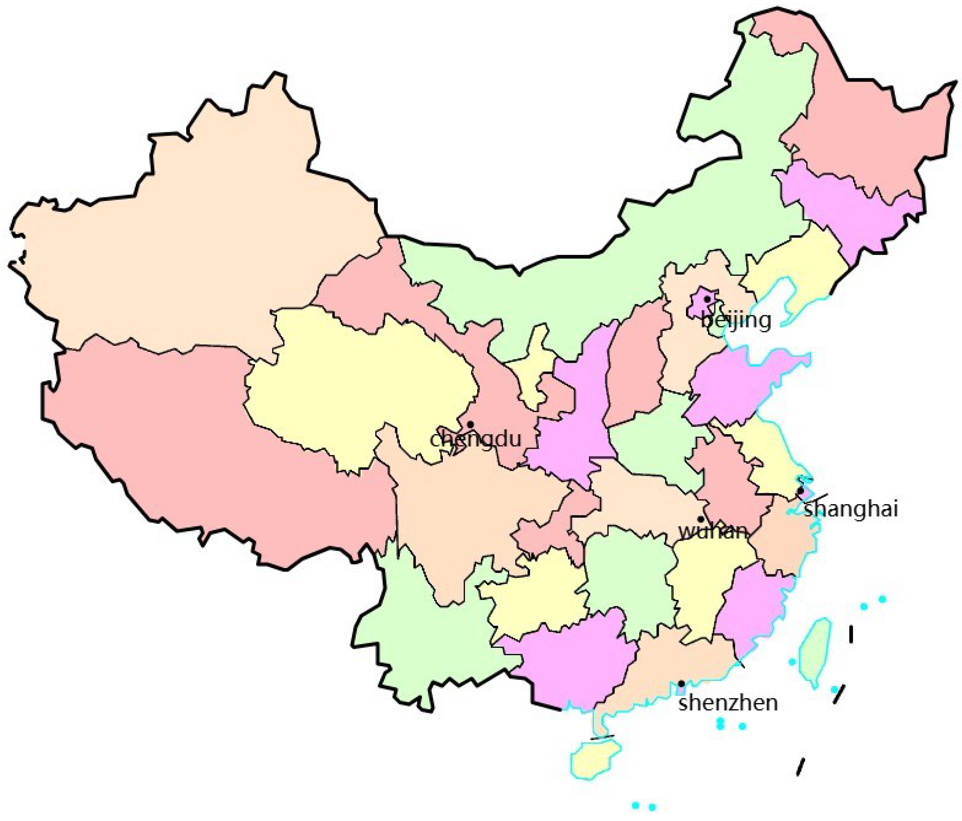
This study selected five cities in China for analysis: Shanghai, Shenzhen, Chengdu, Beijing, and Wuhan. The locations of these cities are shown in
Figure 1. The selection of these cities as the research focus was based on the following reasons and benefits:
Geographical coverage: These five cities are located in distinct regions of China: Shanghai in the east, Shenzhen in the south, Chengdu in the west, Beijing in the north, and Wuhan in the central part of the country. This diverse geographical distribution provided a broader perspective for air quality prediction, ensuring the model was not biased by regional characteristics and enhancing its generalizability across the country.
Diversity of economic and industrial activities: The five cities differ significantly in terms of their economic development and industrial structures. Shanghai and Shenzhen, as economic and industrial hubs, are characterized by high levels of traffic and industrial emissions. Beijing, influenced by its winter heating systems, Chengdu, with its unique geographical and industrial landscape, and Wuhan, representing the central region of China, each presenting distinct pollution sources. This diversity allowed for a comprehensive investigation of the impact of various air pollution factors on air quality.
Climate diversity: The climate types in these cities vary widely. Shanghai and Shenzhen have a humid climate, Beijing experiences a continental monsoon climate, Chengdu is situated in a basin climate, and Wuhan has a subtropical monsoon climate. The differences in climate affect air quality in unique ways, enabling the model to incorporate a wide range of climatic influences and enhancing its ability to adapt to varying weather conditions.
2.2. Data Collection
This study used daily data (data spanned a daily period) from the China Air Quality Online Monitoring and Analysis Platform, covering a 5-year period from 30 September 2019, to 30 September 2024, for cities throughout China, with a total of 1829 data points. The dataset included the average levels of six pollutants monitored at all air quality monitoring stations in each city: , , , , , and . Additionally, the average value of the Air Quality Index (AQI) was recorded for each monitoring station. According to the “Ambient Air Quality Standards” (GB 3095-2012), the concentration data for each pollutant were determined based on the hourly average values.
The AQI is a widely used indicator for assessing air quality in many countries. The primary benchmarks for AQI measurement include the standards set by the US Environmental Protection Agency (EPA), the European Union (EU), the World Health Organization (WHO), as well as national standards of China and other countries [
22]. Although these standards are largely similar in terms of calculation methods for the AQI and the 0–500 scale range, they differ in the average measurement periods for various pollutants and the allowable concentration thresholds over time, which results in variations between the standards. The main reasons behind these discrepancies lie in the differing objectives of the standards and the strategies adopted by policymakers. In general, compared to China’s national standards, the EPA and EU standards specify lower allowable concentrations of pollutants and lower AQI threshold values. While EPA standards are widely accepted globally, China maintains its own national AQI standards, which diverge in several aspects. China’s AQI formula is as follows:
where
C is the real-time concentration of the pollutant,
is the upper limit of the corresponding concentration interval,
is the lower limit of the corresponding concentration interval,
is the upper limit of the corresponding sub-index, and
is the lower limit of the corresponding sub-index. We calculated the
of each pollutant and took the maximum value as the AQI value:
2.3. Data Preprocessing
Due to equipment malfunctions, extreme weather conditions, and other factors, there were a small number of missing values in the collected data. Since the quantity of missing data was minimal, and considering that the Air Quality Index (AQI) is a time-series dataset, linear interpolation was employed to fill in the missing values by interpolating between adjacent data points.
The collected data were tested for normality using the Shapiro–Wilk test, which is a commonly used method to assess whether a dataset follows a normal distribution. The Shapiro–Wilk test is particularly suitable for small sample sizes (typically less than 2000 data points) and is widely used in statistics and data science to validate the assumption of normality. By examining the test statistic and p-value, we could determine whether the data significantly deviated from a normal distribution.
The Shapiro–Wilk test statistic measures the goodness-of-fit between the observed data and a normal distribution. A value closer to 1 indicates a better fit to the normal distribution. The
p-value is used to test the null hypothesis that the data follow a normal distribution. A commonly used significance level is 0.05. If the
p-value is greater than 0.05, we fail to reject the null hypothesis, meaning the data are normally distributed. Conversely, if the
p-value is less than or equal to 0.05, we reject the null hypothesis, indicating that the data do not follow a normal distribution. Based on the test results presented in
Table 1, it was found that the data did not follow a normal distribution.
2.4. Gaussian Filtering
Due to various factors, the collected data exhibited high variance, which presented a challenge for machine learning models. One common type of noise found in the data was random or white noise, which is inherently unpredictable. To address this issue, several noise reduction techniques have been proposed, with one of the most well-known and straightforward methods being the application of frequency-domain filters. These filters process the frequency components of a signal, thereby providing valuable insights into the structure and behavior of the signal.
Gaussian filtering [
23] is a linear filtering technique commonly used for smoothing images, with the goal of reducing noise and fine details. It is widely applied in image processing and computer vision, where it smooths the image by calculating a weighted average of neighboring pixels. The weights for this average are determined by a Gaussian function (i.e., a normal distribution). This method effectively preserves the overall structure of the image while removing noise. In addition to its applications in image processing, Gaussian filtering also plays a significant role in time-series analysis, particularly for data smoothing, noise reduction, and handling non-stationary data.
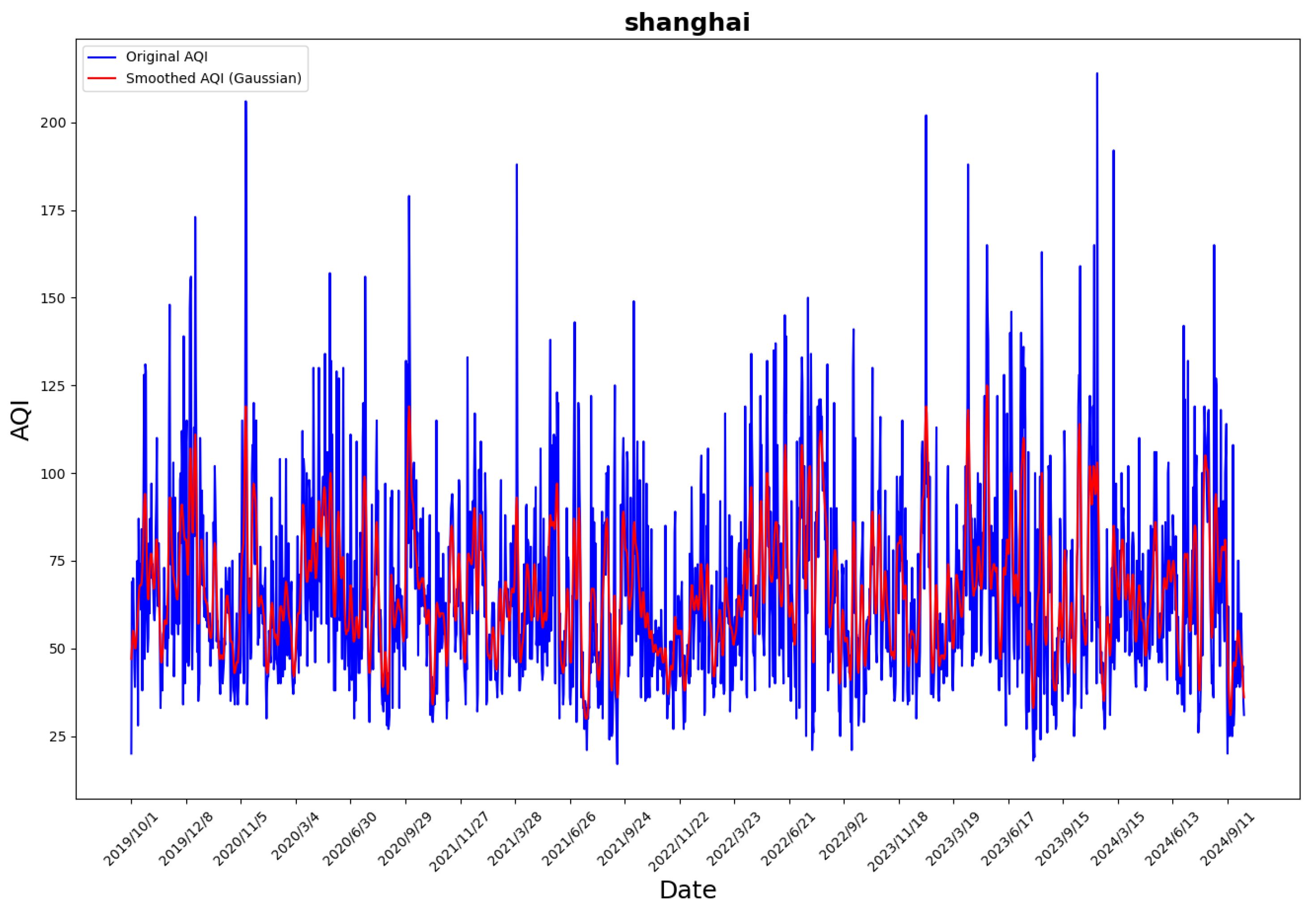
While Gaussian filtering is traditionally used in image processing, its noise-reduction and smoothing capabilities are equally applicable to time-series data. In this study, a Gaussian filter with a variance of 2 was applied to process the AQI feature in the dataset. The comparison between the original AQI data and the Gaussian-filtered AQI is shown in
Figure 2. The filtering process can be expressed by the following formula:
2.5. Min–Max Normalization
In data processing and machine learning, to enable better comparison, it is common practice to scale the original data by adjusting the minimum value to and the maximum value to 1, with other values proportionally scaled between these two extremes. This technique is referred to as feature scaling, or more specifically, Min–Max normalization.
Min–Max normalization transforms the original data features into a specific range, typically between and 1, based on the minimum and maximum values of the data. This scaling technique ensures that the features are proportionally adjusted within the desired range, facilitating more effective comparison and integration with machine learning models.
The formula for Min–Max normalization is as follows:
where
X is the original data feature value,
is the minimum value of the feature,
is the maximum value, min and max are scaled to range from −1 to 1.
2.6. Evaluation Metrics
This study used four indicators to evaluate the prediction effect of the model, namely,
,
,
, and
. Their formulas are as follows:
where
is the real value;
is the predicted;
n is sample size; and
is the mean of the samples. The primary distinction between Mean Absolute Error (MAE) and Mean Absolute Percentage Error (MAPE) stems from their error quantification methodologies and domain-specific applicability. The MAE computes the absolute deviation between predicted and observed values, expressed in the original data unit. It exhibits robustness to outliers, accommodates zero-valued observations, and is preferred in scenarios prioritizing absolute error magnitude (e.g., inventory management systems). However, its lack of scale invariance hinders direct comparisons across heterogeneous datasets. The MAPE, by contrast, quantifies relative error as a percentage of the observed value, providing scale-agnostic interpretability (e.g., “5% deviation”). This metric facilitates cross-dimensional performance benchmarking (e.g., sales volume vs. user growth predictions) and aligns with business communication standards. Nevertheless, the MAPE suffers from two critical limitations: (i) mathematical indefiniteness when actual values equal zero and (ii) asymmetric error amplification for small-denominator observations, which systematically biases predictions towards underestimation. To establish a rigorous dual evaluation framework, this study adopted both MAE and MAPE as complementary performance metrics. Their synergistic application enabled the holistic assessment of model accuracy across absolute and relative error dimensions, thereby mitigating individual metric biases and enhancing interpretative robustness.
2.7. Research Methodology
2.7.1. Convolutional Neural Network
CNN (Convolutional Neural Network) Convolutional Neural Networks (CNNs) are a class of deep learning models originally designed for image and visual tasks but that have since been widely adopted across various domains [
24]. CNNs utilize a layered architecture composed of convolutional layers and pooling layers, which work together to progressively extract hierarchical spatial features from input data. The key components of a CNN include the following layers:
Convolutional layer: This layer applies convolution operations using filters (or kernels) to the input data, extracting local features. Convolution essentially performs a local weighted summation, where each filter is designed to detect different features in the input data. This process enables the network to learn spatial hierarchies of features [
25].
Activation function: Nonlinear activation functions, such as ReLU (Rectified Linear Unit), are applied to the output of the convolutional layer to introduce nonlinearity into the model. This enhances the network’s capacity to model complex patterns and relationships in the data.
Pooling layer: The pooling layer, typically placed after convolutional layers, reduces the dimensionality of the data through downsampling, which helps decrease computational load and provides translation invariance for the features. Common pooling techniques include Max Pooling and Average Pooling, which retain the most important features while reducing the overall size of the data.
Fully connected layer: After the convolutional and pooling layers extract high-level features, these are usually passed to a fully connected layer for classification or regression tasks. The fully connected layer connects every node from the previous layer to all nodes in the current layer, enabling the model to learn more complex decision boundaries within the feature space.
In this study, the traditional fully connected layer was replaced with KANs (Kolmogorov–Arnold Networks), which offer enhanced capabilities for modeling complex, nonlinear relationships in the data.
2.7.2. Long Short-Term Memory
Long Short-Term Memory (LSTM) networks are a specialized type of Recurrent Neural Network (RNN) that are particularly effective at capturing long-term and short-term dependencies in time-series data [
26]. LSTM addresses the issues of vanishing and exploding gradients found in traditional RNNs, making it more suitable for handling long sequences of data.
The core of an LSTM unit is its gating mechanism, which controls the flow of information, allowing it to retain long-term dependencies while discarding irrelevant data. An LSTM unit consists of the following gates:
Forget gate: The forget gate decides which information should be “forgotten” or retained from the cell state. It takes the current input and the previous hidden state to compute the output, which represents the proportion of information to keep or discard. The equation for the forget gate is as follows:
where
is the output of the forget gate, indicating the proportion to be retained or forgotten (value between 0 and 1).
and
are the weight and bias parameters of the forget gate, and
is the sigmoid function.
Input gate: The input gate controls which new information is allowed to be added to the cell state. It includes two components: Candidate cell state
, which generates new candidate information at the current moment.
is the bias term for the candidate cell state, used to adjust the generation of the candidate state and control the intensity of new information generation.
Input gate
determines which parts of the candidate cell state will be added to the current cell state.
is the bias term for the input gate, used to adjust the activation level of the input gate and control how much new information is added.
Then, it updates the cell state:
where
is the current cell state, which represents the important information of the sequence data up to the current moment. The output gate determines the hidden state
at the current moment. It is used to output the result of the current time step and also as one of the inputs of the next time step. The calculation formula is as follows:
where
is the output of the output gate, which controls which part of the cell state information is output.
is the hidden state at the current moment, which is passed to the next time step as the output of LSTM.
is the bias term for the output gate, used to adjust the activation level of the output gate and control how much information is output to the hidden state.
LSTM networks are particularly useful for time-series data, where they can learn long-term trends and seasonal variations, which is critical for tasks like AQI prediction. In this study, the LSTM network processed features extracted by the CNN and performed further time-series modeling. Stacking multiple layers of LSTM enhanced the model’s representational power, enabling it to capture more complex temporal patterns.
2.7.3. Kolmogorov–Arnold Networks
Kolmogorov–Arnold Networks (KANs) [
27] are a type of neural network based on the Kolmogorov–Arnold Superposition Theorem, designed to approximate complex high-dimensional functions by decomposing them into lower-dimensional mappings and their combinations. The formula for the KAN generally follows the Kolmogorov Superposition Theorem, which asserts that any continuous function can be represented as a finite sum of continuous functions and their linear combinations. For any continuous function
, it can be expressed as a linear combination of finitely many continuous functions
and
, that is:
In the KAN model, a network is constructed to approximate complex high-dimensional mappings using multiple nonlinear transformations. The architecture of a KAN is typically implemented through a Multi-Layer Perceptron (MLP) that employs nonlinear activation functions (such as ReLU, sigmoid, or tanh) to approximate the target function. In practice, the KAN architecture optimizes the model parameters to minimize expected errors, adjusting them to better approximate the desired function.
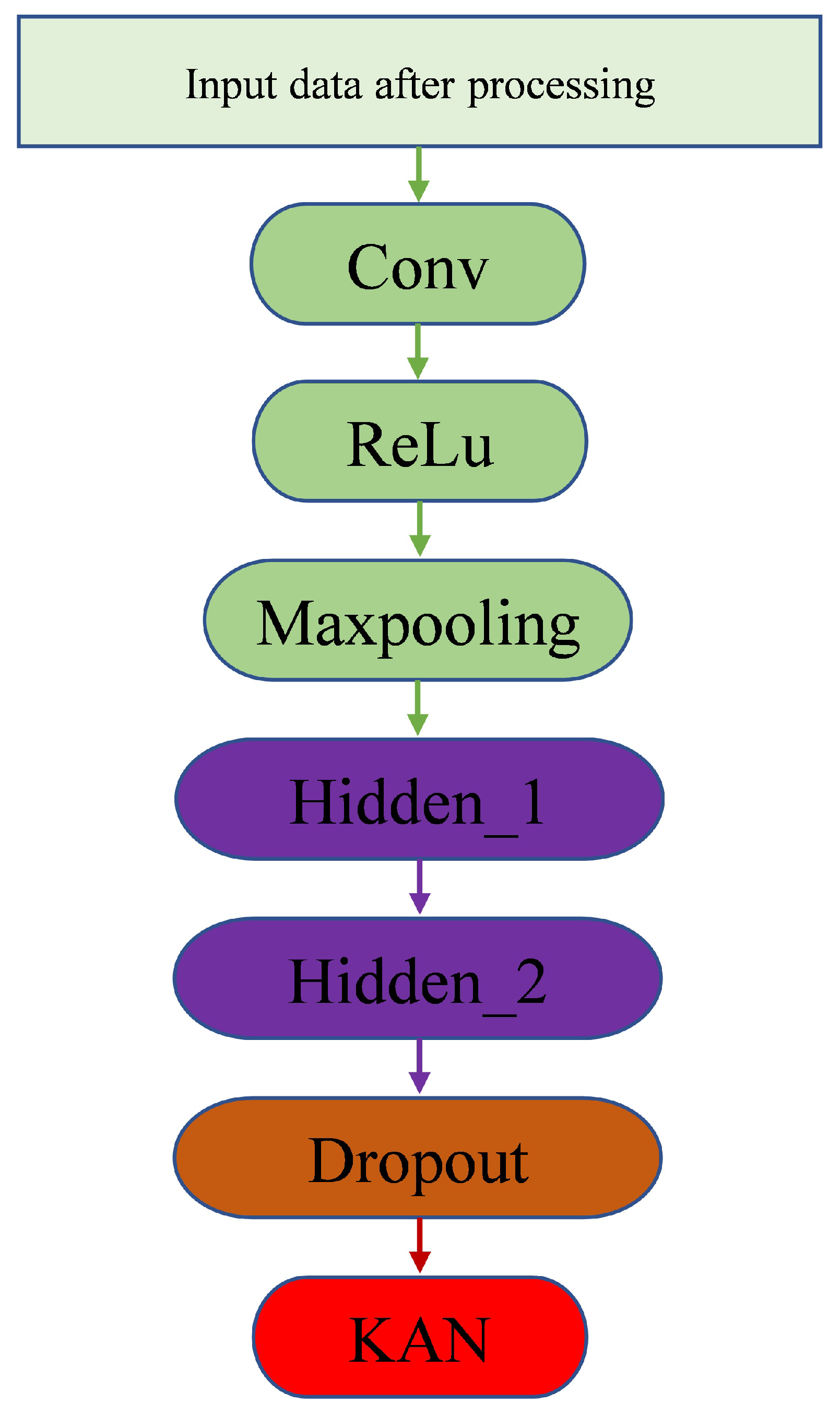
In this study, a KAN was used as a module following the LSTM layers, replacing traditional fully connected layers. While conventional fully connected layers map features to output spaces through linear transformations, a KAN uses a more sophisticated structure to integrate features from different layers, thereby capturing the nonlinear relationships in the data more effectively. Specifically, a KAN enhances the model’s generalization ability, reduces overfitting, and better handles the nonlinear relationships inherent in time-series data. The introduction of the KAN module aimed to overcome the limitations of traditional LSTM models, boosting the model’s capacity to learn from complex temporal data. By incorporating the KAN module at the final stage of the model, the network could leverage higher-dimensional features, leading to more accurate AQI predictions. The hybrid model structure is illustrated in
Figure 3.
2.8. Model Construction and Training
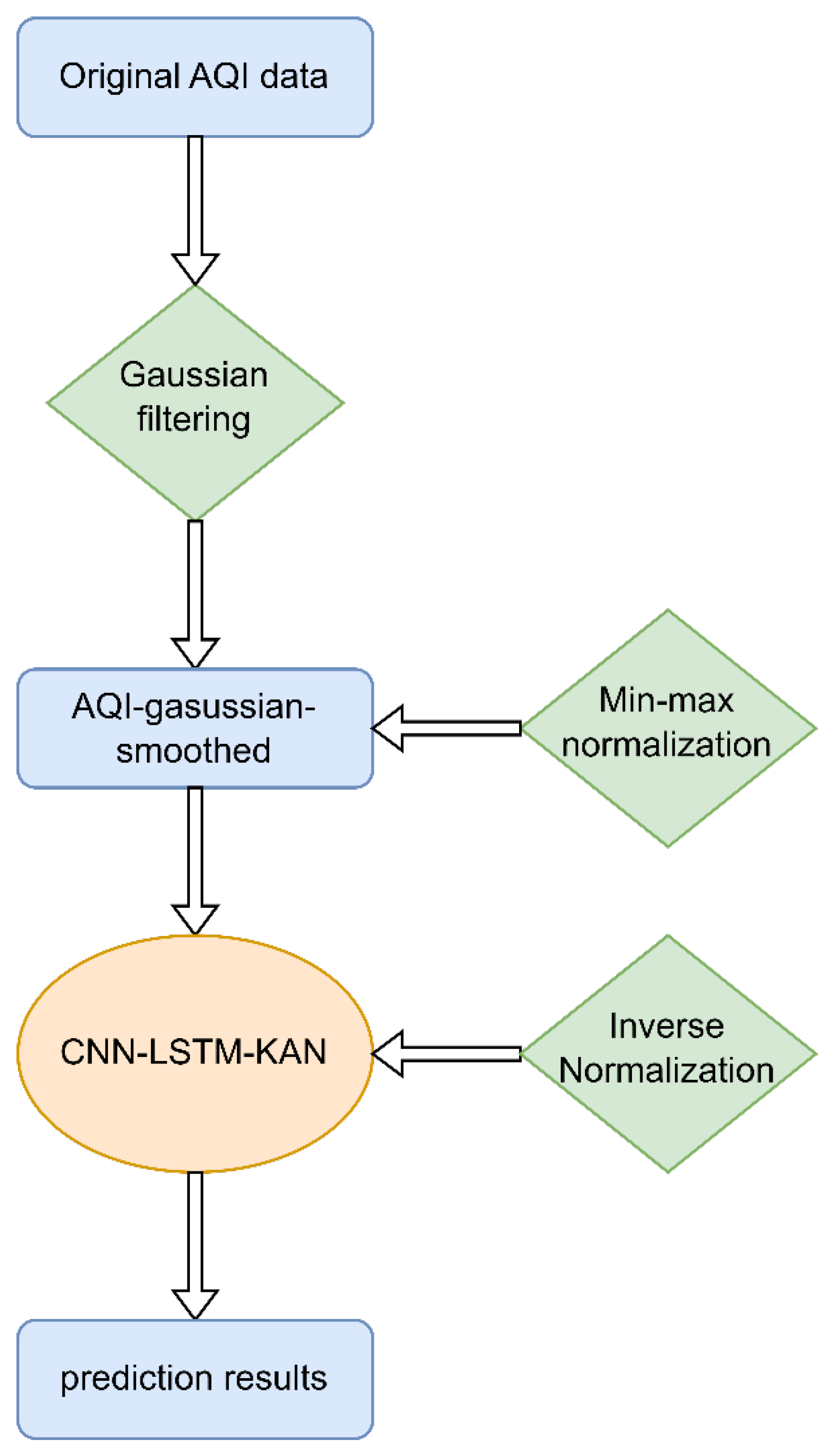
In this study, the model combined a Convolutional Neural Network (CNN), Long Short-Term Memory (LSTM) network, and Kolmogorov–Arnold Network (KAN) to predict the Air Quality Index (AQI) (The training set and the test set were divided in a ratio of 8:2). The core structure of the model consisted of multiple layers designed to efficiently extract features from time-series data and capture both short-term and long-term temporal dependencies. The hybrid model’s training and prediction process is illustrated in
Figure 4. Below is a detailed description of the model architecture:
The first part of the model was the Convolutional Neural Network (CNN), which was used to extract local features from the AQI time-series data. The CNN was designed to adapt to the temporal nature of the data, focusing on capturing time-based patterns and trends within the daily AQI sequence. This was achieved using specialized 1D convolutional layers that detected temporal patterns and trends in the AQI data.
The input data first passed through a 1D convolutional layer with a kernel size of 3, one input channel, and 32 output channels [
28]. The convolutional layer applied a sliding-window operation over the input sequence to extract local temporal features. The result of these convolution operations was a feature map that contained the local temporal correlations within the AQI data. A ReLU activation function was then applied to introduce nonlinearity and enhance the model’s expressive capability. Following this, a Max Pooling layer was used to reduce the dimensionality of the feature map while retaining the essential temporal features. This helped reduce computational complexity and prevent overfitting. The extracted features were then passed to the LSTM layer.
The LSTM layer was responsible for capturing both short-term and long-term dependencies in the time-series data. In this model, the LSTM layer consisted of 32 hidden units and was configured with two layers. The LSTM utilized its memory cell (cell state) to process temporal relationships within the sequence, enabling it to capture complex dynamic changes in the AQI data over time. The LSTM is unidirectional, meaning it generates predictions progressively, moving from past time steps toward future predictions.
To prevent overfitting, a dropout layer was introduced with a dropout rate of 0.2. Dropout works by randomly deactivating a fraction of neurons, forcing the network to learn more robust feature representations, which improves the model’s generalization ability. After the LSTM layer, a Kolmogorov–Arnold Network (KAN) was incorporated. The KAN used kernel methods to learn the significance of features and assign different weights to them, thereby emphasizing critical moments in the AQI sequence. This allowed the model to focus more precisely on key time periods, enhancing prediction accuracy. The input to the KAN layer was the output from the LSTM layer, and the output of the KAN layer generated the final prediction.
During training, the model used the Mean Squared Error (MSE) as the loss function, and the Adam optimizer was used to update the model parameters. The learning rate (lr) for the Adam optimizer was set to 0.01, which helped accelerate the convergence process. The model’s parameters were adjusted via backpropagation at each training epoch to minimize the loss function.
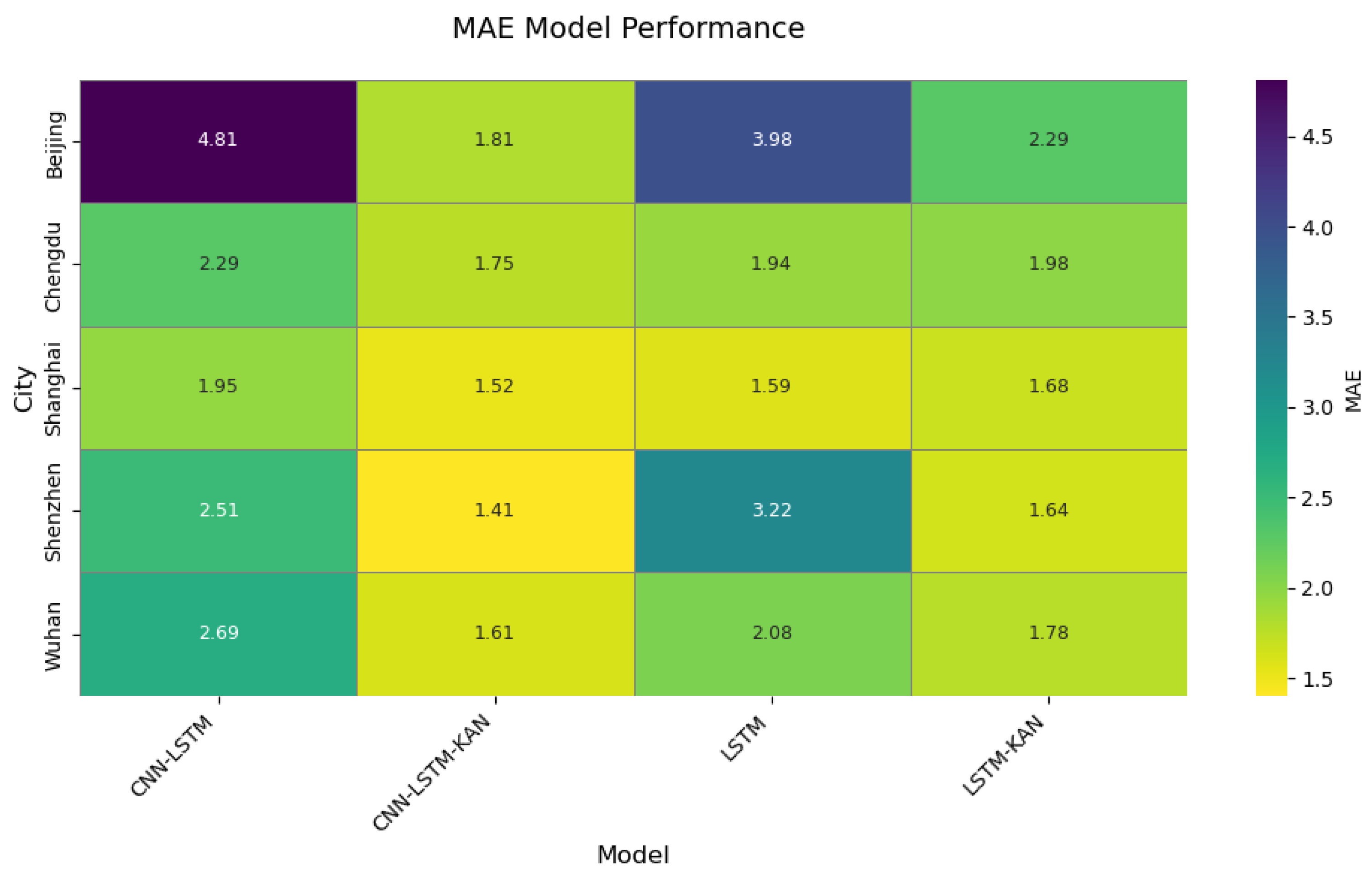
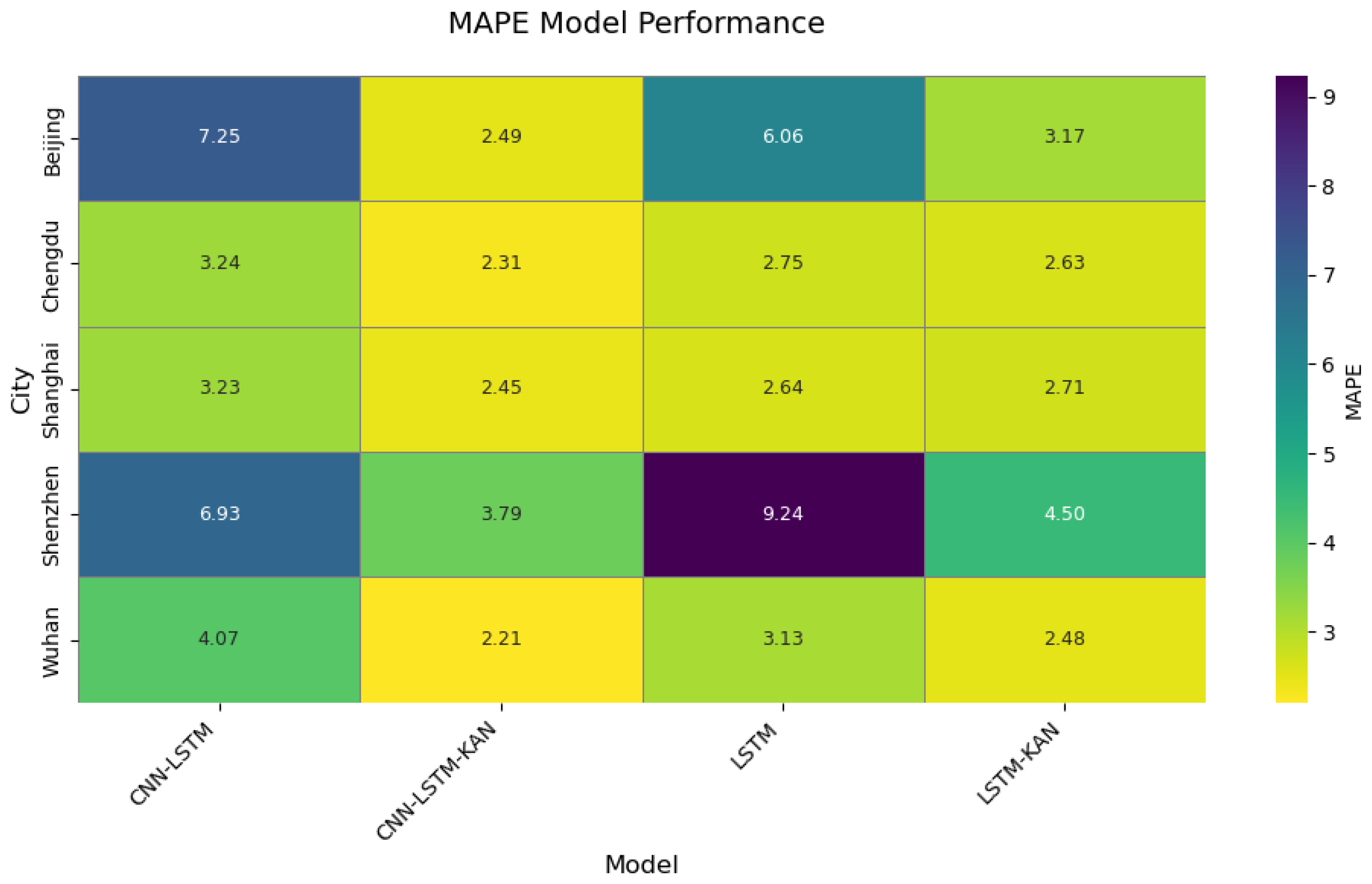
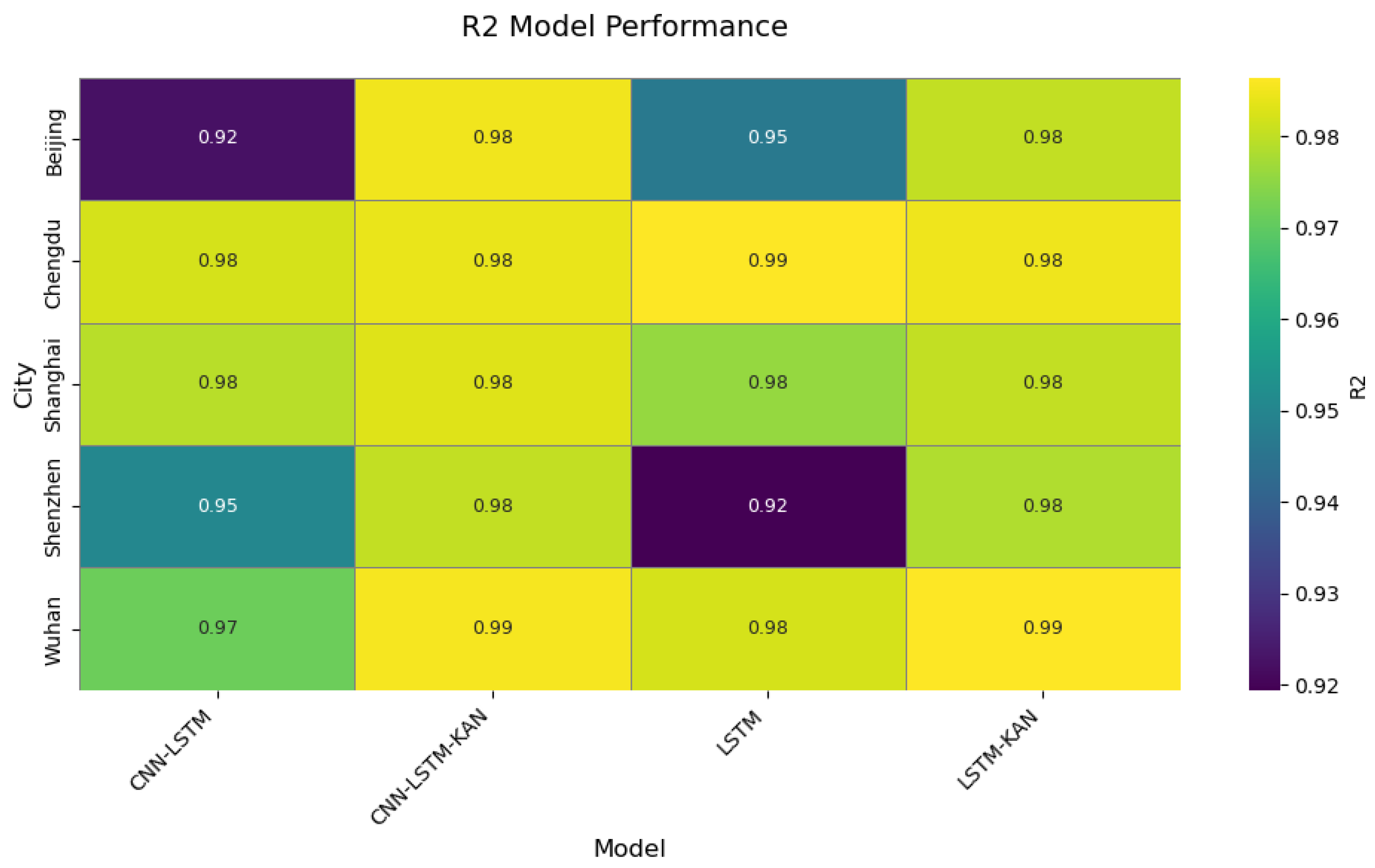
The model was trained over 200 epochs, with the training loss recorded at each epoch to optimize the parameters. After training, the model’s performance was validated using a test set. The evaluation metrics included the Root-Mean-Square Error (RMSE), R2, Mean Absolute Error (MAE), and Mean Absolute Percentage Error (MAPE). These metrics assessed the model’s prediction accuracy, explanatory power, and robustness across different datasets.
The model’s input consisted of preprocessed AQI time-series data. During preprocessing, the data were first denoised using Gaussian filtering and then normalized using MinMaxScaler to scale it to the range of [, 1]. The training and test sets were split in an 80:20 ratio, and the data were divided into different time windows. Each time window typically contained the past 20 days of data (lookback = 20) to predict future AQI values. The output was the predicted AQI, which was then reverse-normalized to the original scale for comparison with the actual data.
After model training was complete, several evaluation metrics were used to test its performance. First, the RMSE was calculated for both the training and test sets to assess prediction accuracy. A lower RMSE value indicated more accurate predictions. Next, R2 was used to evaluate the model’s ability to explain the variance in the data. A higher R2 value signified better explanatory power. Additional metrics such as MAE and MAPE further validated the model’s robustness across different datasets.
In summary, this model combined a CNN for local feature extraction, LSTM for capturing temporal dependencies, and a KAN for enhancing key feature learning. This hybrid approach enabled the model to effectively predict the AQI and served as a high-precision tool for air quality monitoring.
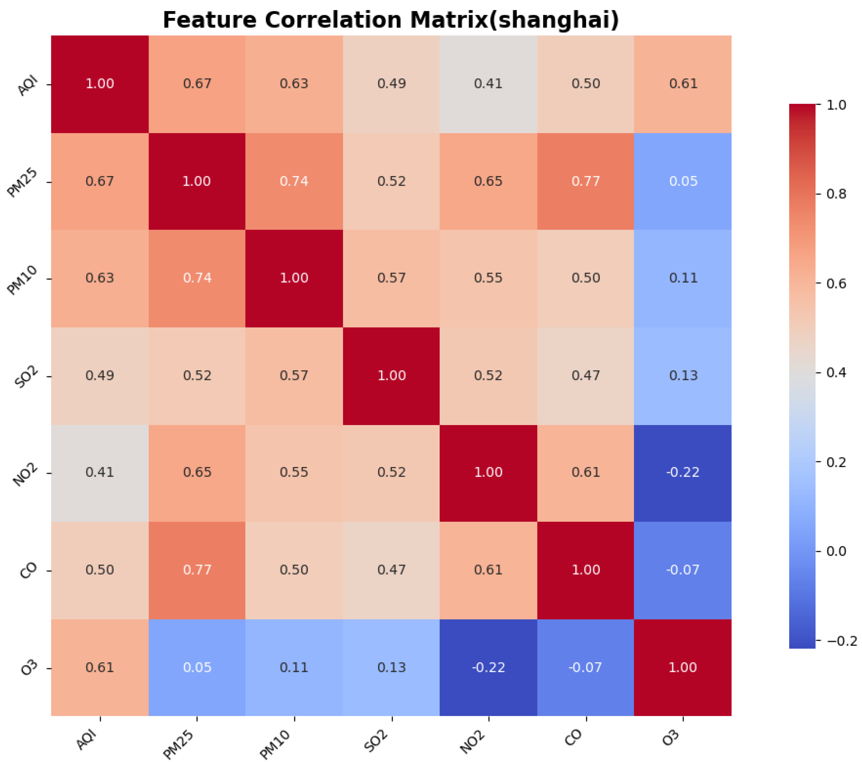
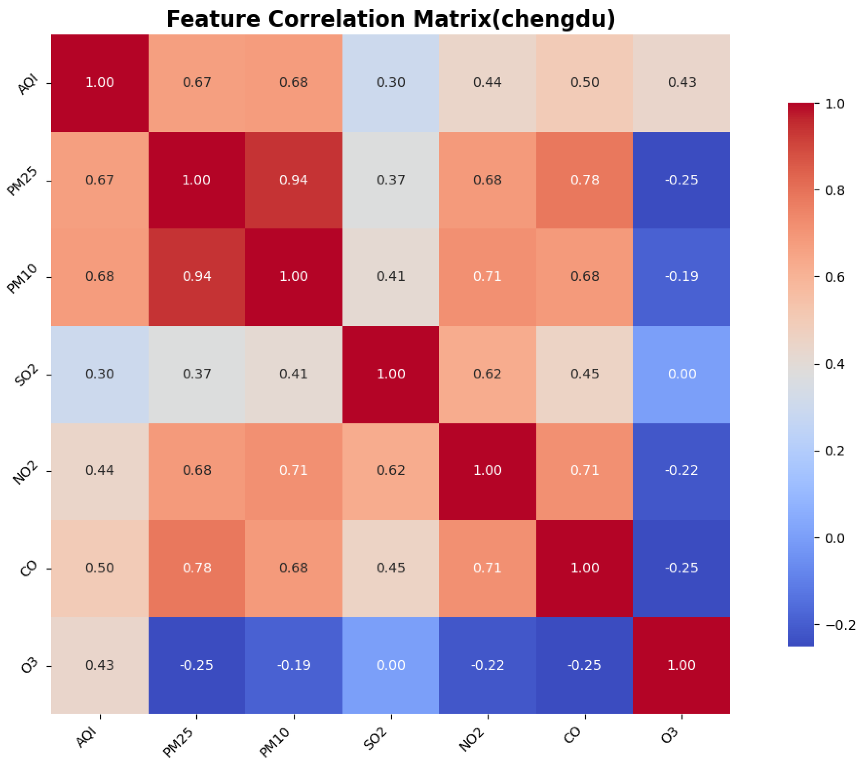
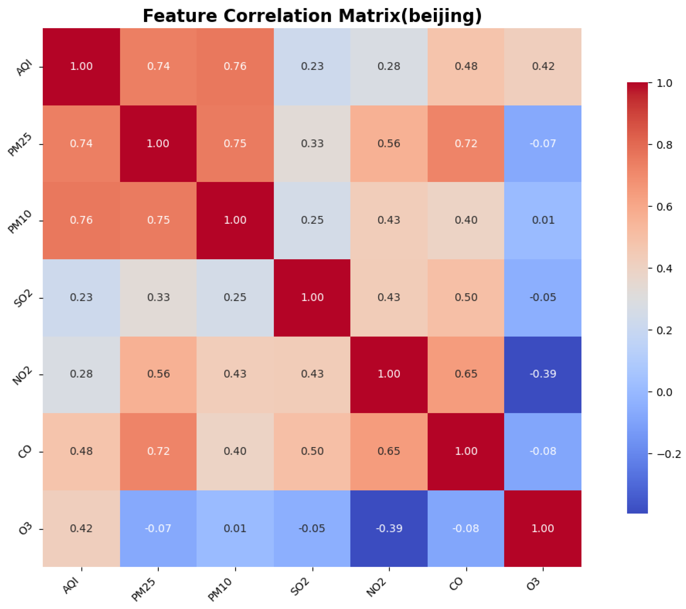
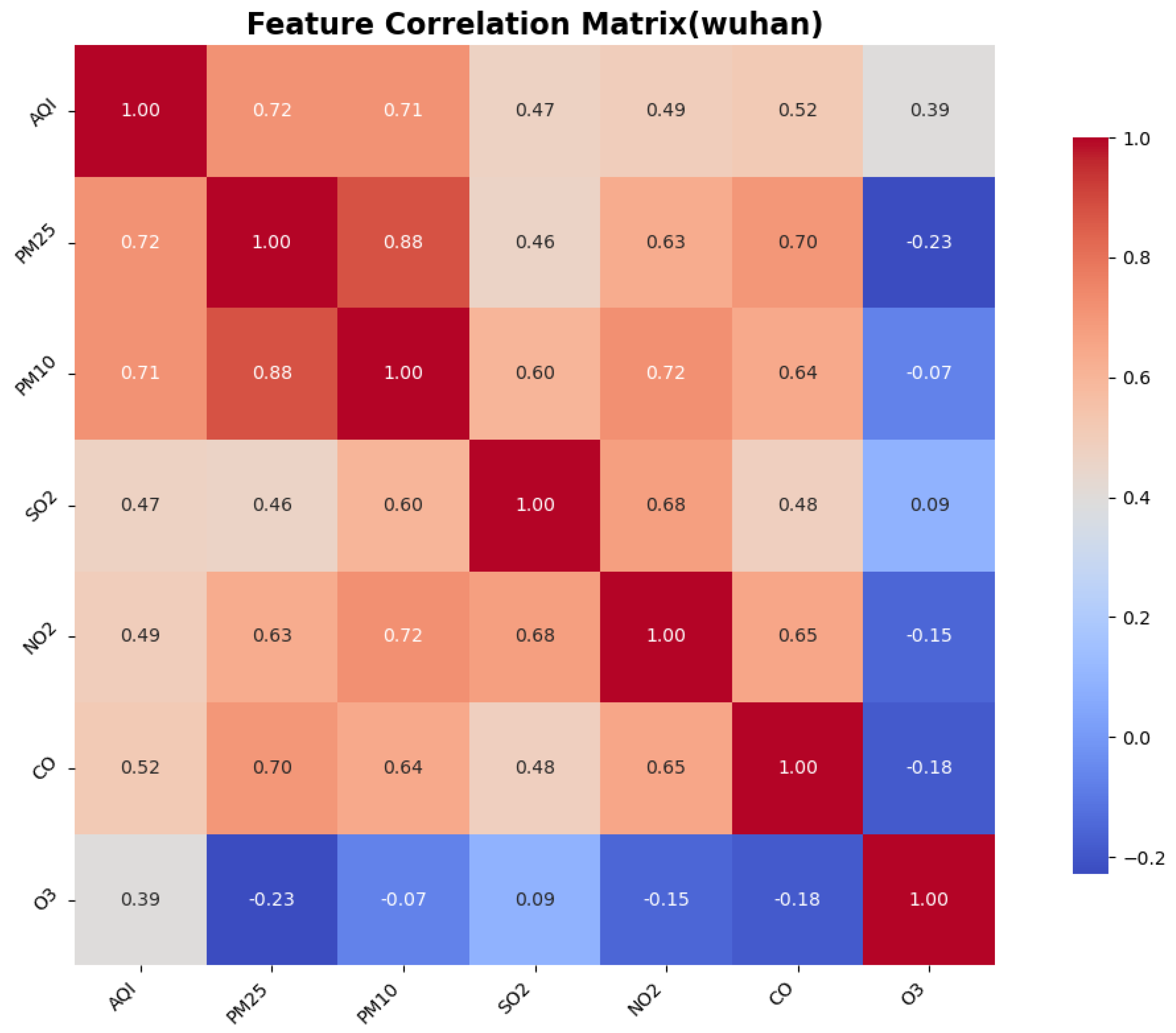
2.9. Correlation Analysis
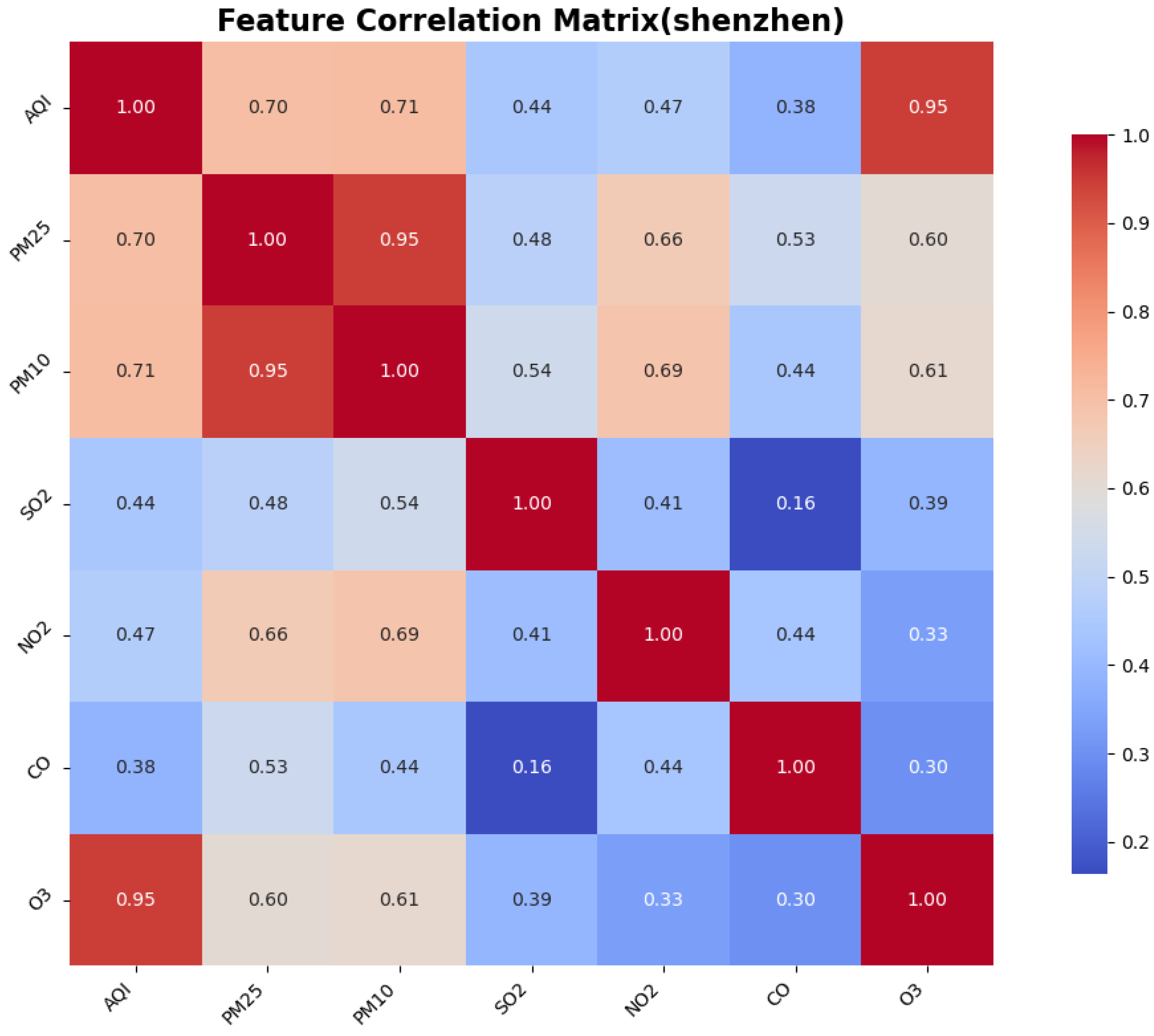
To identify the similarities and differences in pollution patterns across various cities in China and to explore the deeper relationships between the Air Quality Index (AQI) and other air pollutants, we calculated the correlations between features, particularly focusing on the correlation between the AQI and the other pollutants. This was accomplished using a correlation matrix, which helped to identify the most significant features for AQI prediction.
The Pearson correlation coefficient test is a statistical method used to assess the strength and direction of the linear relationship between two variables. It quantifies the correlation between two variables using the Pearson correlation coefficient, which ranges from to 1. This method is widely employed in scientific research, social sciences, and data analysis to determine whether significant correlations exist between variables. The correlation between AQI and the other six features is illustrated in the figure.
The formula is as follows:
where
and
represent the values of the two variables, and
and
represent the means of the two variables. The range of
r is (
, 1).
4. Conclusions
Air quality prediction plays an integral role in monitoring and predicting pollution levels, contributing significantly to urban sustainability. Given the growing concerns regarding air pollution, accurate prediction of air quality is essential for timely decision-making and urban management. This study addressed the critical challenge of air quality prediction in heterogeneous environments through the development of a CNN-LSTM-KAN hybrid deep learning framework, yielding three key theoretical contributions:
1. Methodological innovation in data governance: The non-Gaussian distribution characteristics of air quality data, validated by Shapiro–Wilk testing (p < 0.05), informed the development of an integrated preprocessing framework combining Gaussian filtering with Min–Max normalization. This approach significantly enhanced model convergence speed and noise suppression efficacy.
2. Architectural breakthrough in model design: The novel integration of Kolmogorov–Arnold Networks (KANs) with attention mechanisms, replacing conventional fully connected layers, established a dynamic feature weighting system that demonstrated superior complex pattern recognition capabilities. Comparative experiments revealed the model’s RMSE reductions of 59.6–44.7% against baseline LSTM in representative cities (Beijing and Shenzhen), with R2 values reaching 0.92–0.99.
3. Environmental heterogeneity decoding: cross-city validation identified PM2.5/PM10 as universal dominant predictors (correlation coefficients: 0.76–0.89), while simultaneously detecting ozone sensitivity in coastal cities like Shenzhen, providing theoretical foundations for region-specific pollution control strategies.
Practical implementation value: The proposed framework successfully overcame the generalization limitations of conventional models in spatiotemporally heterogeneous environments. The synergistic combination of multi-scale feature extraction (CNN-LSTM modules) and dynamic feature reconstruction (KAN modules) established an extensible technical foundation for smart-city air quality warning systems. The model’s differentiated performance in high-variability (e.g., Shenzhen) and high-pollution scenarios (e.g., Beijing) confirmed its strong adaptability to complex urban ecosystems. While significant progress has been achieved, four critical directions warrant further investigation: (1) Multimodal data fusion: integration of spatiotemporal covariates including meteorological parameters and traffic patterns to develop coupled natural-social system prediction paradigms. (2) Computational efficiency optimization: creation of lightweight Transformer-based architectures enhanced with federated learning for multi-city collaborative prediction.


