Can GCMs Simulate ENSO Cycles, Amplitudes, and Its Teleconnection Patterns with Global Precipitation?

Abstract

The ability of a general circulation model (GCM) to capture the variability of El Niño–Southern Oscillation (ENSO) is not only a scientific issue of climate model performance, but also critical for climate change and variability impact studies. Here, we assess 48 CMIP5 GCMs for their skill in simulating ENSO interdecadal variability and its teleconnection with precipitation globally. The results show that (1) only 22 out of 48 GCMs display interdecadal variability that is similar to the observations; (2) the ensemble of the 48 GCMs captures the ENSO–precipitation teleconnection at the global scale; (3) no single GCM can capture the observed ENSO–precipitation teleconnection globally; and (4) a GCM that can realistically simulate ENSO variability does not necessarily capture the ENSO-precipitation teleconnection, and vice versa. The results could also be used by climate change impact studies to select suitable GCMs, especially for regions with a statistically significant teleconnection between ENSO and precipitation, as well as for the comparison of CMIP5 and CMIP6.

1. Introduction

It is well documented that ENSO is a dominant driver of climate (precipitation and temperature) [1,2,3] and streamflow [4,5] variability, as well as their extreme events such as drought [6], in many locations throughout the world, and its teleconnection provides the scientific basis for long-range weather forecasts. On the other hand, general circulation models, or global climate models (GCMs), are the primary tools to simulate present climate and probably the best available models to project future climate for given greenhouse gas emission scenarios and pathways [7]. The outputs of GCMs are useful for understanding future global climatic changes and for assessing the impact of future climate on processes of interest [8]. Therefore, the ability of a GCM to capture ENSO variability and its relationship with precipitation is not only a scientific issue of climate model performance, but also critical for climate change and variability impact studies, e.g., water resource management to cope with projected climate change and variability.

Numerous studies have investigated ENSO variability and its impact on precipitation using GCMs. For example, Lin [9] assessed the interdecadal variability of ENSO with 21 Intergovernmental Panel on Climate Change (IPCC) Fourth Assessment Report (AR4) or phase 3 of the Coupled Model Intercomparison Project (CMIP3) GCMs, and found that the GCMs displayed a wide range of skills in simulating the interdecadal variability of ENSO. Jin et al. [10] investigated the overall skill of ENSO predictions in retrospective forecasts made with ten CMIP3 coupled GCMs. They concluded that the simulation of the interannual SST variability was far from perfect in most coupled models and the forecast skill of individual GCM depends strongly on season, ENSO phase, and ENSO intensity. Neelin and Langenbrunner [11] analyzed the ENSO–precipitation (December to February, or DJF) teleconnection in 15 CMIP5 and 13 CMIP3 GCMs for 1979–2005. They showed that within regions of strong observed teleconnections between ENSO and precipitation, there was little improvement from the CMIP5 ensemble relative to CMIP3 in amplitude and spatial correlation metrics of precipitation. Jiang et al. [12] examined whether 16 GCMs and 10 RCMs could represent the multi-scale temporal variability of observed station data in the southwestern United States. They found that the GCMs/RCMs tended to simulate longer storm duration and lower storm intensity in comparison with those from observed records. Rowell [13] provided an overview of the state of the art modelling of SST teleconnections to Africa. King et al. [14] investigated the ENSO–Australia precipitation teleconnection in reanalysis and CMIP5 GCMs and concluded that some GCMs captured the asymmetric nature of the ENSO–rainfall relationship (the magnitude of La Niña events has a greater effect on rainfall than does the magnitude of El Niño events) whilst others do not. Kristóf et al. [15] evaluated the historical simulations of GCMs based on detected atmospheric teleconnections and concluded that major teleconnection patterns are similar for GCMs and reanalysis datasets; however, spatial differences in their intensities were severe in some cases. Yin et al. [6] investigated the combined impacts of ENSO and Indian Ocean Dipole (IOD) on global seasonal droughts. Zhao et al. [16] quantified overlapping and differing information of global precipitation for GCM forecasts and ENSO. The results confirmed the effectiveness of GCMs in capturing the ENSO-related variability in global precipitation and illustrated where there is room for improvement of GCM forecasts. Yeh er al. [3] reviewed the ENSO atmospheric teleconnections and their response to greenhouse gas forcing, including the changes in ENSO teleconnection patterns that have affected their predictability and the statistics of extreme events.

However, no studies in the literature have investigated ENSO–precipitation teleconnection of CMIP5 GCMs globally, which is the objective of this study. It is investigated in two parts: first, we use the normalized Fourier spectrum of Lin [9] to explore the cycles and amplitudes of ENSO for 48 CMIP5 GCMs. This is an update of Lin’s CMIP3 GCM analysis [9]. Secondly, we investigate the ENSO–precipitation relationship by correlation analysis and by the precipitation anomalies at different phases of ENSO, i.e., La Niña and El Niño episodes [17]. The results could be used to select suitable GCMs for global and regional studies on climate change and variability impacts, especially for regions with a statistically significant correlation between ENSO and regional precipitation.

2. Materials and Methods

2.1. Datasets

Three types of data are used in this study:

(a)

Observed sea surface temperature (SST) datasets to derive ENSO indices. Two different SST datasets are used in this study: the Extended Reconstruction of SST (ERSST) [18], and the Met Office Hadley Centre’s Sea Ice and SST (HADISST) [19]. They are chosen because previous studies with AR4 (CMIP3) models used them [9].

(b)

GCM data. A total of 48 CMIP5 GCMs are used in this study, and their names, acronyms, country, and horizontal and vertical resolutions are listed in

Table 1. The 48 GCMs used in this study.

GCM	Institute	Lat	Lon
ACCESS1-0	The Centre for Australian Weather and Climate Research (Commonwealth Scientific and Industrial Research Organisation, CSIRO, and Bureau of Meteorology, BoM)	145	192
ACCESS1-3		145	192
bcc-csm1-1	Beijing Climate Centre, China Meteorological Administration	64	128
bcc-csm1-1-m		160	320
BNU-ESM	Beijing Normal University	64	128
CanESM2	Canadian Centre for Climate Modelling and Analysis	64	128
CCSM4	National Center for Atmospheric Research, USA	192	288
CESM1-BGC	National Science Foundation, Department of Energy, National Center for Atmospheric Research, USA	192	288
CESM1-CAM5-1-FV2		96	144
CESM1-CAM5		192	288
CESM1-FASTCHEM		192	288
CESM1-WACCM		96	144
CMCC-CESM	Centro Euro-Mediterraneo per I Cambiamenti Climatici	48	96
CMCC-CM		240	480
CMCC-CMS		96	192
CNRM-CM5-2	Centre National de Recherches Meteorologiques/Centre Europeen de Recherche et Formation Avancees en Calcul Scientifique	128	256
CNRM-CM5		128	256
CSIRO-Mk3-6-0	Commonwealth Scientific and Industrial Research Organisation	96	192
EC-EARTH	EC-EARTH consortium	160	320
FGOALS-g2	LASG, Institute of Atmospheric Physics, Chinese Academy of Sciences; and CESS, Tsinghua University	60	128
FGOALS-s2	LASG, Institute of Atmospheric Physics, Chinese Academy of Sciences	108	128
FIO-ESM	The First Institute of Oceanography, SOA, China	64	128
GFDL-CM2p1	Geophysical Fluid Dynamics Laboratory, USA	90	144
GFDL-CM3		90	144
GFDL-ESM2G		90	144
GFDL-ESM2M		90	144
GISS-E2-H-CC	NASA Goddard Institute for Space Studies, USA	90	144
GISS-E2-H		90	144
GISS-E2-R-CC		90	144
GISS-E2-R		90	144
HadCM3	Met Office Hadley Centre, UK	73	96
HadGEM2-AO		145	192
HadGEM2-CC		145	192
HadGEM2-ES	Met Office Hadley Centre (Realizations contributed by Instituto Nacional de Pesquisas Espaciais)	145	192
inmcm4	Institute for Numerical Mathematics	120	180
IPSL-CM5A-LR	Institut Pierre-Simon Laplace	96	96
IPSL-CM5A-MR		143	144
IPSL-CM5B-LR		96	96
MIROC-ESM-CHEM	Japan Agency for Marine-Earth Science and Technology, Atmosphere and Ocean Research Institute (The University of Tokyo), and National Institute for Environmental Studies	64	128
MIROC-ESM		64	128
MIROC5	Atmosphere and Ocean Research Institute (The University of Tokyo), National Institute for Environmental Studies, and Japan Agency for Marine-Earth Science and Technology	128	256
MPI-ESM-LR	Max Planck Institute for Meteorology (MPI-M)	96	192
MPI-ESM-MR		96	192
MPI-ESM-P		96	192
MRI-CGCM3	Meteorological Research Institute, Japan	160	320
MRI-ESM1		160	320
NorESM1-ME	Norwegian Climate Centre	96	144
NorESM1-M		96	144

.

(c)

Observed global precipitation. The Global Precipitation Climatology Centre (GPCC) monthly precipitation is used in this study. It comprises gridded datasets interpolated based on quality-controlled data from 67,200 stations globally [20]. For ENSO interdecadal variability, monthly data covering 115 years (1890–2004) are used because a few CMIP5 GCM historical runs end in 2004. The ENSO–precipitation teleconnection analysis is limited to 1950–2004 for two reasons: (1) to be consistent with National Weather Service La Niña and El Niño episodes by (http://www.cpc.ncep.noaa.gov/products/analysis_monitoring/ensostuff/ensoyears.shtml, accessed on 30 September 2024), which started in 1950, and (2) because the quality of precipitation data in the early 1950s is relatively poor due to a limited number of stations.

2.2. Methods

The interdecadal variability, i.e., cycles and amplitudes, of ENSO is investigated with the normalized Fourier spectrum. The power spectra, or power spectral densities, are estimated with the sine multitaper approach of Riedel and Sidorenko [21] through the R package “psd: Adaptive, sine multitaper power spectral density estimation for R” [22]. The sum of densities is set to 1 to normalize it.

The ENSO–precipitation relationship is investigated by a correlation analysis and precipitation anomalies at different phases of ENSO, i.e., La Niña and El Niño episodes [17]. The temporal correlation coefficients between Niño3.4 SST anomalies and annual precipitation at every 1° by 1° land grid are used. Only regions or grids with a temporal correlation coefficient which is statistically significant at the α = 0.05 level are reported. It is tested with the statistic:

$$t={\displaystyle \frac{r}{\sqrt{\frac{1-r^2}{n-2}}}},$$

(1)

distributed approximately as a t-distribution with a degree of freedom n − 2. r is the correlation coefficient, and n is the number of years.

The long-term monthly precipitation is averaged for every 1° land grid based on three categories: La Niña, El Niño, and neutral episodes [17]. The sum of monthly precipitation from January to December is treated as “annual” precipitation in La Niña, El Niño, and neutral events, so the numbers of months to be averaged will vary given the different lengths of three episodes. For example, for the La Niña episode, there are 16 Januarys but only 4 Julys from the ACCESS1-0 model. The “annual” precipitation anomalies for La Niña/El Niño are then used to explore their differences. The definition of the National Weather Service is adopted in this study based on the SST anomalies for the Niño3.4 region: a La Niña (El Niño) episode can be said to occur if the 3-month running means of SST anomalies in the Niño 3.4 region (averaged between 5° N and 5° S, 170° W and 120° W) are below −0.5 °C (exceed 0.5 °C) for a minimum of 5 consecutive over-lapping seasons. A month which is neither within a La Niña or El Niño episode is then defined as a neutral episode. In order to remove the warming trend, moving 30-year base periods are used to define the SST anomaly. These 30-year base periods are used to calculate the anomalies for successive 5-year periods in the historical record: the anomaly during 1950–1955 will be based on the 1936–1965 base period, and the values during 1956–1960 will be based on the 1941–1970 base period, and so on (http://www.cpc.ncep.noaa.gov/products/analysis_monitoring/ensostuff/ensoyears.shtml, accessed on 30 September 2024).

3. Results

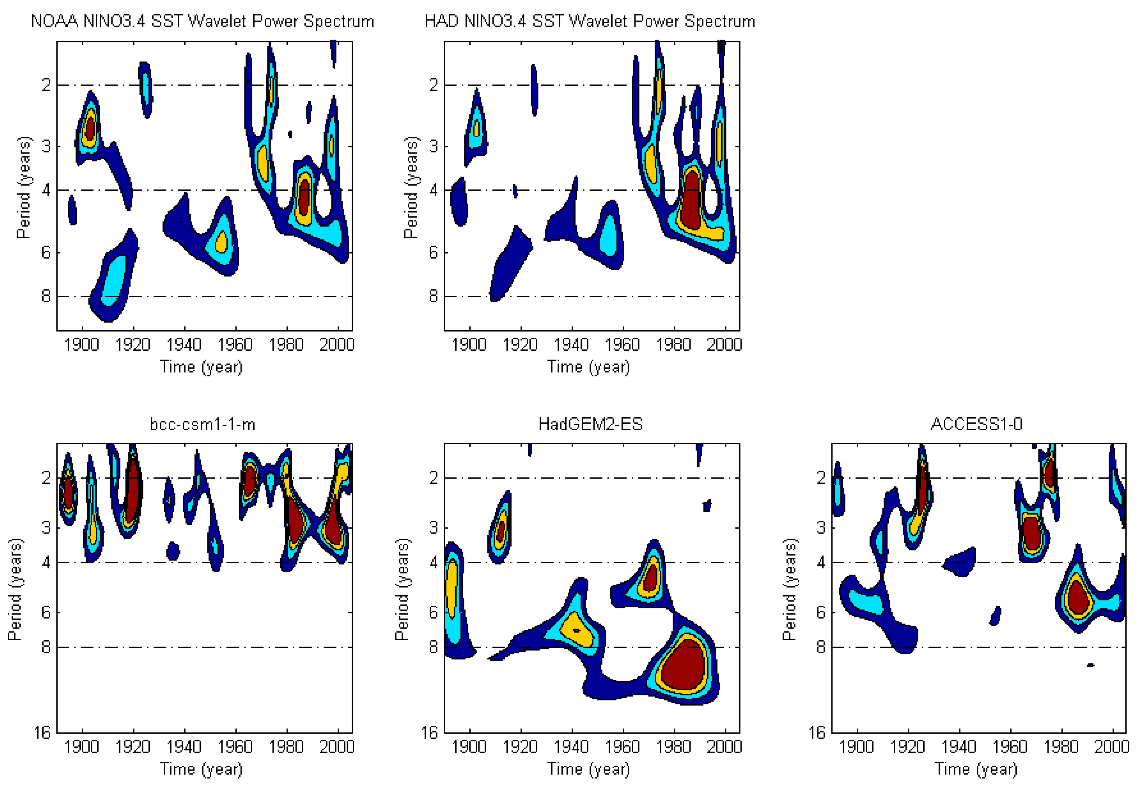
3.1. Interdecadal Variability of ENSO

The normalized Fourier spectra of the Niño3.4 SST in both observations (red and blue lines) and the 48 CMIP5 GCMs (black lines) are shown in Figure 1. The observed ENSO shows a broadband signal with two spectral peaks between 3 and 7 years (two vertical grey lines). The 48 GCMs can be categorized into four groups:

(a)

Seven GCMs displayed a pronounced spectral peak with a period shorter than the observed ENSO period (first row);

(b)

Nine GCMs produced one prominent peak with a period longer than 7 years (second row);

(c)

Ten GCMs displayed a spectral peak that is similar to an ENSO-like 3–7-year period, but with a larger amplitude (third row);

(d)

The remaining twenty-two GCMs displayed a relatively good spectral peak with a 3–7-year period as well as a similar amplitude to the observed one (fourth row).

A caveat on these groupings is that the category boundaries are subjectively judged by visual inspection. For example, GISS-E2-H-CC, as plotted in Figure 2, sits between groups (a) and (d).

This conclusion is confirmed with the results of a wavelet analysis [23,24] (Figure 3): both observations, NOAA NINO3.4 SST and HAD (Met Office Hadley Centre) NINO3.4 SST, show a wavelet spectrum of 3–7 years, and their frequences over time in the past 100 years are also identical. This is additional information in terms of frequency components in both time and frequency, in comparison to the Fourier spectrum analysis (Figure 1). On the other hand, the bcc-csm1-1m GCM displayed a shorter period of 2–4 years and it was consistent in the past 100 years; HadGEM2-ES showed a longer period of 7–12 years; and ACCESS1-0 displayed the same 3–7-year period as the observations.

There is an improvement in CMIP5 over CMIP3 models in terms of the dominant period and its amplitude. Only 8 out of 21 CMIP3 GCMs, or 38%, had a similar ENSO variability as the observations [9], compared to 46% (22 out of 48) for the CMIP5 GCMs. This is consistent with existing studies. For example, Bellenger et al. [25] showed that the ENSO amplitude exhibits less diversity in CMIP5 than in CMIP3: 65% of CMIP5 model ENSO amplitude falls within 25% of the observed value against 50% for CMIP3; the ENSO cycle is also slightly improved in CMIP5, although the CMIP5 multi-model ensemble does not improve greatly compared to CMIP3. Zhang et al. [26] also showed a modest improvement in the CMIP5 simulations of ENSO-SSTA meridional width over CMIP3 models.

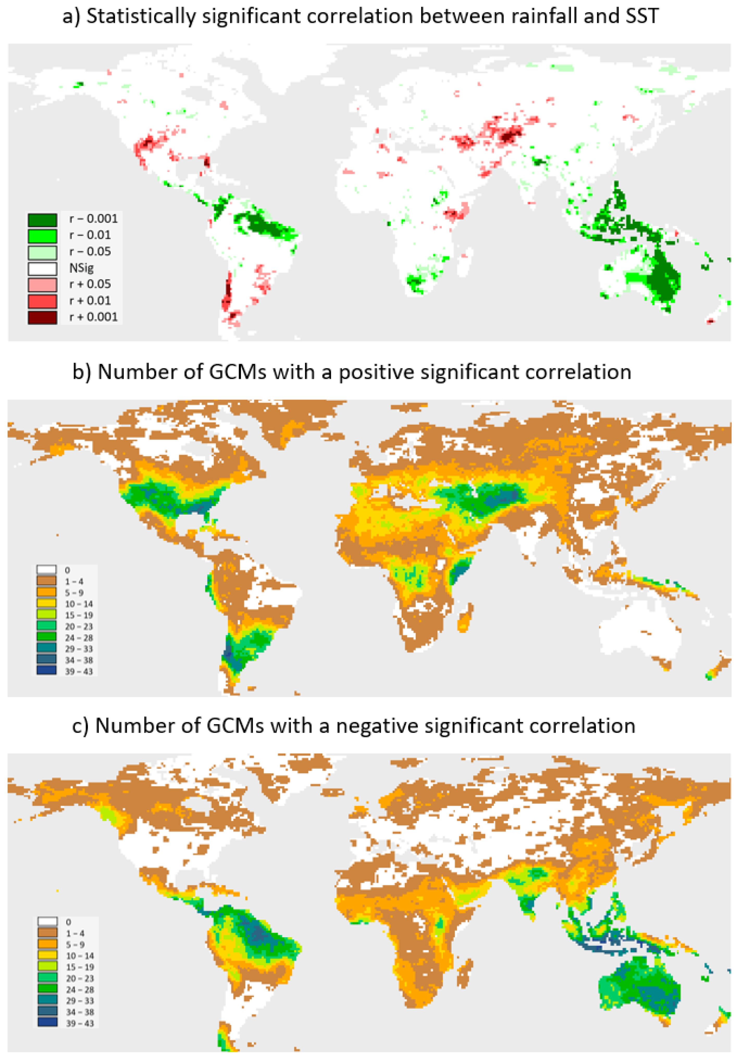
3.2. ENSO–Precipitation Teleconnections

Overall, the ensemble of 48 GCMs (Figure 4, second and third rows in comparison to the first row) can capture the ENSO–precipitation teleconnection at the global scale, showing the four statistically significant positive centers in east Africa, the Middle East, southern USA, and the southern portion of South America (first and second rows), as well as three of the four statistically significant negative centers in Indonesia, Australia, and the northern portion of South America (first and third rows). This conclusion is expected as the CMIP5 multi-model ensemble provides a conservative estimate of local/regional trends in precipitation [27]. However, very few GCMs simulated the teleconnection in South Africa and a large number of GCMs simulated a teleconnection in southern India where the observations do not show such a teleconnection.

Figure 5 shows the correlation coefficients between annual precipitation and Niño3.4 SST, and the precipitation anomalies (%) during the La Niña and El Niño episodes of 1950 to 2004 from the observations and four GCMs selected to show the range of possible responses, i.e., ACCESS1-3 (the same signs of statistically significant correlation coefficient, and the same positive/negative precipitation anomaly during the La Niña/El Niño episodes for Australia as those observed), CESM1-CAM5 (statistically insignificant correlation coefficients and little precipitation anomalies during La Niña/El Niño episodes), MRI- ESM1 (an opposite precipitation anomaly to that observed for southeastern Australia during the La Niña/El Niño episodes and, accordingly, a statistically insignificant correlation coefficient), and GFDL-ESM2M (an overestimation of areas with statistically significant correlation coefficients and precipitation anomalies). Supplementary File S2 presents the correlation coefficients and the precipitation anomalies during both La Niña and El Niño episodes for all 48 GCMs.

Unfortunately, none of the 48 GCMs can capture all of these correlations and anomalies at the global scale (Figure 6 and

Table 2. Numbers (observations, GPCC) and percentage of cells (48 GCMs) with precipitation anomaly (P) during La Niña/El Niño episodes.

GCMs	Coincident Precipitation Anomaly				Non-Coincident Precipitation Anomaly
	La Niña		El Niño		La Niña		El Niño
	P > 110%	P < 90%	P > 110%	P < 90%	P > 110%	P < 90%	P > 110%	P < 90%
GPCC	1962	1229	1463	1833
ACCESS1-0	40.9	41.6	42.9	35.3	32.4	113.8	99.6	47.0
ACCESS1-3	36.1	43.3	48.2	44.5	36.1	86.7	82.6	50.4
bcc-csm1-1	32.8	18.2	11.8	21.4	31.4	76.6	49.1	15.3
bcc-csm1-1-m	28.6	37.8	47.2	29.9	22.5	95.9	78.3	29.7
BNU-ESM	59.8	35.2	35.3	57.8	57.2	73.1	48.4	55.0
CanESM2	44.7	57.2	63.7	48.9	60.8	133.8	90.2	71.0
CCSM4	44.2	39.6	52.2	48.6	43.7	77.5	71.2	49.0
CESM1-BGC	31.9	31.1	46.1	42.2	43.2	49.3	54.8	37.9
CESM1-CAM5-1-FV2	44.5	53.2	58.1	56.4	51.7	97.7	78.3	54.3
CESM1-CAM5	0.7	9.5	1.6	1.1	6.8	17.6	3.9	13.9
CESM1-FASTCHEM	45.9	31.9	43.7	33.3	41.1	65.6	51.5	37.0
CESM1-WACCM	49.3	43.0	47.2	54.4	47.0	60.2	55.5	58.9
CMCC-CESM	52.7	30.8	57.7	53.9	50.1	55.6	99.3	48.4
CMCC-CM	33.6	49.1	30.4	17.2	54.9	172.5	76.1	30.0
CMCC-CMS	54.7	56.4	62.4	43.8	27.4	116.7	104.2	27.3
CNRM-CM5-2	45.2	42.1	46.9	24.5	36.4	86.1	86.1	19.0
CNRM-CM5	32.8	44.1	45.4	26.2	20.2	66.2	66.4	16.7
CSIRO-Mk3-6-0	60.6	41.2	56.9	54.1	79.0	102.3	100.1	74.0
EC-EARTH	23.1	10.5	16.0	11.7	48.2	41.7	22.2	8.3
FGOALS-g2	35.1	26.1	23.3	33.8	16.7	60.6	52.4	19.1
FGOALS-s2	56.5	38.5	32.7	37.0	62.1	116.1	68.5	39.0
FIO-ESM	49.6	40.4	36.2	38.1	40.6	82.3	51.7	36.2
GFDL-CM2p1	58.7	51.2	60.2	67.2	79.9	98.4	100.1	92.0
GFDL-CM3	36.2	51.1	46.3	39.2	29.9	98.6	72.4	28.8
GFDL-ESM2G	50.6	49.4	47.1	43.0	48.1	104.1	71.5	30.9
GFDL-ESM2M	56.3	67.7	81.3	50.5	68.3	136.2	147.9	88.3
GISS-E2-H-CC	38.9	32.8	7.4	23.6	38.5	107.4	23.9	25.5
GISS-E2-H	21.3	26.8	30.7	8.3	24.4	84.9	74.8	15.3
GISS-E2-R-CC	19.3	21.0	7.9	15.8	46.9	79.1	19.9	40.8
GISS-E2-R	11.9	18.1	20.1	11.9	21.8	61.8	57.3	37.2
HadCM3	26.8	46.2	23.0	33.0	33.3	96.4	36.6	44.6
HadGEM2-AO	44.7	43.4	20.4	35.4	56.8	98.4	63.0	37.0
HadGEM2-CC	32.2	27.8	23.8	23.2	46.2	76.6	37.2	43.3
HadGEM2-ES	32.1	28.5	28.9	19.5	39.3	74.3	51.5	22.5
inmcm4	32.3	20.4	14.4	34.6	51.5	69.3	36.9	48.8
IPSL-CM5A-LR	44.6	40.2	23.8	37.8	51.7	97.6	53.5	41.1
IPSL-CM5A-MR	42.2	28.9	35.5	42.8	53.4	64.5	92.6	83.1
IPSL-CM5B-LR	28.6	48.7	54.3	18.3	33.4	160.2	147.7	20.3
MIROC-ESM-CHEM	32.2	6.1	16.8	44.6	69.7	46.9	40.3	128.5
MIROC-ESM	16.5	9.9	7.9	28.5	81.1	62.6	34.9	63.3
MIROC5	46.3	32.6	74.8	46.8	37.8	79.3	105.3	67.5
MPI-ESM-LR	54.0	47.8	40.2	46.1	41.1	82.5	59.1	36.1
MPI-ESM-MR	53.7	58.5	38.3	48.0	27.0	117.7	83.3	40.5
MPI-ESM-P	4.0	21.7	16.4	17.1	16.6	66.4	39.5	28.3
MRI-CGCM3	16.2	55.9	38.6	23.0	45.8	175.9	94.1	30.6
MRI-ESM1	34.0	42.5	40.2	22.2	69.6	156.6	114.2	34.4
NorESM1-ME	48.7	37.6	39.5	48.8	48.5	69.6	55.8	39.4
NorESM1-M	40.6	34.7	42.1	48.9	54.0	77.8	52.2	38.0

). The coincident correlation coefficient and precipitation anomaly, i.e., the percentage of global land areas where a GCM can successfully simulate the statistically significant correlation coefficients and the positive/negative precipitation during La Niña/El Niño episodes to observations, ranges from 0.7% to 81.3% with a mean and median value of 35–40% (Figure 6 and Table 2).

Overall, GCMs cannot simulate the ENSO–precipitation teleconnection for 60–65% of global land areas where the observations show such a teleconnection. In contrast, a GCM can simulate a statistically significant correlation coefficient and a positive/negative precipitation anomaly during the La Niña/El Niño episodes for a specific region, but where the observations do not show such a teleconnection. This is defined as non-coincident correlation coefficient and precipitation anomaly. Unfortunately, this ranges from 3.9% to 314.8% (percentage of observed coincidence area). The mean and median values vary with correlation coefficient, positive/negative precipitation anomaly, and La Niña/El Niño episodes (Figure 6 and Table 2). For example, they are 89.2% and 82.4% for the negative precipitation anomaly during La Niña episodes, and 42.6% and 37.9% for the negative precipitation anomaly during El Niño episodes (Figure 6 and Table 2).

CESM1-CAM5 (Figure 5, third row) shows very little ENSO–precipitation teleconnection during both La Niña and El Niño episodes for Australia, as well as for the global precipitation. Its areas of coincident precipitation anomalies are only 0.7%, 9.5%, 1.6%, and 1.1% for the positive/negative precipitation anomaly during La Niña and El Niño episodes, respectively (Table 2). It is interesting to note that CAM5 is given a modest score for ENSO links to Australia in the Climate Change in Australia project (http://www.climatechangeinaustralia.gov.au/, accessed on 12 March 2025) [28,29], and it is perhaps the best model for climate field assessment [30]. MRI-ESM1, in contrast, has an opposite precipitation anomaly for southeastern Australia during La Niña episodes and for southern Australia during El Niño episodes (Figure 5, fourth row).

It is not surprising that many GCMs overestimate the precipitation anomalies, given the high values of non-coincident precipitation correlation coefficient and precipitation anomaly (Figure 6). For example, GFDL-ESM2M overestimates both ENSO–precipitation teleconnection areas and the magnitude of precipitation anomalies for northern and southern America, northern Africa, southeast Europe, and the Middle East (Figure 5, fifth row). These results indicate that the ENSO–precipitation teleconnection is poorly simulated by the current generation of GCMs globally, although some GCMs do simulate the precipitation responses to ENSO variability for some regions (e.g., Australia). This performance may be partly due to the unpredictable nature of multi-decadal periods of high and low ENSO variability [31].

4. Discussion

4.1. Implications of This Study

ENSO is a dominant driver of climate variability [1,2] and GCMs are the primary tools to simulate present climate and probably the best available models to project future climate for given greenhouse gas emission scenarios and pathways [7]. Therefore, the ability of a GCM to capture ENSO variability and its relationship with precipitation is not only a scientific issue of climate model performance, but also critical for climate change and variability studies, such as the selection of suitable GCMs, especially for regions with a statistically significant teleconnection, in order to explore the impacts of climate change and variability on hydrology and water resources, agriculture, ecology, energy, and health [32].

4.2. Uncertainties and Limitations

4.2.1. CMIP5 vs. CMIP6 GCMs

While 48 CMIP5 GCMs are used in this study, we fully understand that CMIP6 GCM results are available. These new generation GCMs, in theory, should improve climate simulations because of their higher resolution and better representation of physical processes. However, the results of this study are still useful, especially for the comparison of CMIP5 and CMIP6 in terms of ENSO and its teleconnection with precipitation. For example, Liao et al. [33] investigated the bias of the ENSO phase-locking behavior persisting in 42 CMIP6 GCMs and 43 CMIP5 GCMs, and found that there was no difference between CIPM5 and CMIP6 GCMs, with only 12 CMIP5 and 15 CMIP6 being used to simulate ENSO with a majority proportion of winter-peaking events. Brown et al. [34] compared the past and future simulations of ENSO in CMIP5/PMIP3 and CMIP6/PMIP4 models and concluded that no consistent relationship between changes in ENSO amplitude and annual cycle was identified across experiments. Beobide-Arsuaga et al. [35] investigated the uncertainty of ENSO amplitude projections in CMIP5 and CMIP6 models and found that the total uncertainty increased from CMIP5 to CMIP6.

In addition, CMIP6 GCMs seem to underestimate ENSO teleconnections in the Southern Hemisphere [36], which was not seen from the results of this study with CMIP5 GCMs.

4.2.2. Data Quality

Data quality is always the core of scientific research. (a) GPCC rainfall data are used in this study. This is probably one of the best rainfall products with global coverage. But it still has limitations, such as regions with limited weather stations, mismatch of the point rainfall data at weather station with grid rainfall data, and the potential underestimation of rainfall in dry seasons. (b) GCMs have different spatial resolutions and some GCMs are much coarser (Table 1), but we interpolated them to the same 1° by 1° resolution for comparison. This may bring uncertainties and affect the results. (c) Visual inspection was used to separate GCMs into four groups in terms of the normalized Fourier spectra and ENSO periods. In theory, an objective clustering method should be used instead of subjective grouping. In fact, we did test two clustering analysis methods, i.e., hierarchical clustering analysis and self-organizing maps [37]. However, the results are a little hard to explain and not as clear as visual inspection. The main reason could be that there are two dimensions in the normalized Fourier spectra: period and density. Having said that, visual inspection clearly has its own limitations; for example, GISS-E2-H-CC, as plotted in Figure 2, sits between Group 1 and Group 2. (d) There are different definitions of indices of ENSO.

4.2.3. Physical Processes of GCMs

This study investigates how GCMs simulate ENSO cycles and amplitudes, as well as its teleconnections with global precipitation. However, the uncertainties of GCMs, in which physical processes of climate (such as atmospheric dynamics, ocean circulation, and land surface interactions) are represented with mathematical equations and algorithms, are not further explored in terms of why some GCMs can simulate the ENSO characteristics and its teleconnections with global precipitation and others cannot. These include, but are not limited to, discrepancies between GCMs and the real world, limited ability to simulate local-scale physical processes (such as two sides of a mountain), the parameterization and sensitivity of model processes, and their inability to accurately simulate current climate [38]. This is a very important scientific challenge for which further investigation is needed, but it probably is outside the scope of this study.

5. Conclusions

Forty-eight CMIP5 GCMs are used in this study to assess their skill in simulating ENSO interdecadal variability and its teleconnection with precipitation globally. The results indicate that 22 of 48 GCMs display similar interdecadal variability as the observations, and the ensemble of 48 GCMs captures the regional ENSO–precipitation teleconnection at the global scale. However, no single GCM can capture the observed ENSO–precipitation teleconnection globally. Overall, GCMs do not simulate an ENSO–precipitation teleconnection for 60–65% of the globe where there is an observed teleconnection, and they show a significant teleconnection for large areas where the observations do not show a teleconnection. Moreover, a GCM that can realistically simulate ENSO variability does not necessarily capture the ENSO–precipitation teleconnection at global and regional scales, and vice versa.

The results of this study can be further analyzed to explore the ENSO mechanism, especially under global warming scenarios, as it is not clear whether ENSO activity will be enhanced or damped, or if the frequency of events will change in the coming decades [3,31,39], despite considerable progress in understanding the impact of climate change on many of the processes that contribute to ENSO variability. The results could also be used by climate change impact studies to select suitable GCMs, especially for regions with a statistically significant teleconnection, as well as for the comparison of CMIP5 and CMIP6.

References

1. Ropelewski, C.F.; Halpert, M.S. Global and Regional Scale Precipitation Patterns Associated with the El-Nino Southern Oscillation. Mon. Weather. Rev. 1987, 115, 1606–1626. [Google Scholar] [CrossRef]
2. Power, S.; Delage, F.; Chung, C.; Kociuba, G.; Keay, K. Robust twenty-first-century projections of El Nino and related precipitation variability. Nature 2013, 502, 541–545. [Google Scholar] [CrossRef]
3. Yeh, S.W.; Cai, W.; Min, S.; McPhaden, M.J.; Dommenget, D.; Dewitte, B.; Collins, M.; Ashok, K.; An, S.; Yim, B.; et al. ENSO Atmospheric Teleconnections and Their Response to Greenhouse Gas Forcing. Rev. Geophys. 2018, 56, 185–206. [Google Scholar] [CrossRef]
4. Chiew, F.H.S.; McMahon, T.A. Global ENSO-streamflow teleconnection, streamflow forecasting and interannual variability. Hydrol. Sci. J.-J. Des Sci. Hydrol. 2002, 47, 505–522. [Google Scholar] [CrossRef]
5. Ouyang, R.; Liu, W.; Fu, G.; Liu, C.; Hu, L.; Wang, H. Linkages between ENSO/PDO signals and precipitation, streamflow in China during the last 100 years. Hydrol. Earth Syst. Sci. 2014, 18, 3651–3661. [Google Scholar] [CrossRef]
6. Yin, H.; Wu, Z.; Fowler, H.J.; Blenkinsop, S.; He, H.; Li, Y. The Combined Impacts of ENSO and IOD on Global Seasonal Droughts. Atmosphere 2022, 13, 1673. [Google Scholar] [CrossRef]
7. IPCC. Summary for Policymakers. In Climate Change 2023: Synthesis Report. A Report of the Intergovernmental Panel on Climate Change. Contribution of Working Groups I, II and III to the Sixth Assessment Report of the Intergovernmental Panel on Climate Change; Lee, H., Romero, J., Eds.; IPCC: Geneva, Switzerland, 2023; p. 36. [Google Scholar]
8. Fu, G.; Charles, S.P.; Kirshner, S. Daily rainfall projections from general circulation models with a downscaling nonhomogeneous hidden Markov model (NHMM) for south-eastern Australia. Hydrol. Process. 2013, 27, 3663–3673. [Google Scholar] [CrossRef]
9. Lin, J.L. Interdecadal variability of ENSO in 21 IPCC AR4 coupled GCMs. Geophys. Res. Lett. 2007, 34, L12702. [Google Scholar] [CrossRef]
10. Jin, E.K.; Kinter, J.L.; Wang, B.; Park, C.-K.; Kang, I.-S.; Kirtman, B.P.; Kug, J.-S.; Kumar, A.; Luo, J.-J.; Schemm, J.; et al. Current status of ENSO prediction skill in coupled ocean–atmosphere models. Clim. Dyn. 2008, 31, 647–664. [Google Scholar] [CrossRef]
11. Langenbrunner, B.; Neelin, J.D. Analyzing ENSO Teleconnections in CMIP Models as a Measure of Model Fidelity in Simulating Precipitation. J. Clim. 2013, 26, 4431–4446. [Google Scholar] [CrossRef]
12. Jiang, P.; Gautam, M.R.; Zhu, J.; Yu, Z. How well do the GCMs/RCMs capture the multi-scale temporal variability of precipitation in the Southwestern United States? J. Hydrol. 2013, 479, 75–85. [Google Scholar] [CrossRef]
13. Rowell, D.P. Simulating SST Teleconnections to Africa: What is the State of the Art? J. Clim. 2013, 26, 5397–5418. [Google Scholar] [CrossRef]
14. King, A.D.; Donat, M.G.; Alexander, L.V.; Karoly, D.J. The ENSO-Australian rainfall teleconnection in reanalysis and CMIP5. Clim. Dyn. 2014, 44, 2623–2635. [Google Scholar] [CrossRef]
15. Kristóf, E.; Barcza, Z.; Hollós, R.; Bartholy, J.; Pongrácz, R. Evaluation of Historical CMIP5 GCM Simulation Results Based on Detected Atmospheric Teleconnections. Atmosphere 2020, 11, 723. [Google Scholar] [CrossRef]
16. Zhao, T.; Chen, H.; Tian, Y.; Yan, D.; Xu, W.; Cai, H.; Wang, J.; Chen, X. Quantifying overlapping and differing information of global precipitation for GCM forecasts and El Niño–Southern Oscillation. Hydrol. Earth Syst. Sci. 2022, 26, 4233–4249. [Google Scholar] [CrossRef]
17. Trenberth, K.E. The definition of El Nino. Bull. Am. Meteorol. Soc. 1997, 78, 2771–2777. [Google Scholar] [CrossRef]
18. Smith, T.M.; Reynolds, R.W. Improved Extended Reconstruction of SST (1854–1997). J. Clim. 2004, 17, 2466–2477. [Google Scholar] [CrossRef]
19. Rayner, N.A.; Parker, D.E.; Horton, E.B.; Folland, C.K.; Alexander, L.V.; Rowell, D.P.; Kent, E.C.; Kaplan, A. Global analyses of sea surface temperature, sea ice, and night marine air temperature since the late nineteenth century. J. Geophys. Res. Atmos. 2003, 108, 4407. [Google Scholar] [CrossRef]
20. Schneider, U.; Becker, A.; Finger, P.; Meyer-Christoffer, A.; Rudolf, B.; Ziese, M. GPCC Full Data Reanalysis Version 6.0 at 1.0°: Monthly Land-Surface Precipitation from Rain-Gauges Built on GTS-Based and Historic Data. 2011. Available online: https://cir.nii.ac.jp/crid/1883679867557616512 (accessed on 30 September 2024).
21. Riedel, K.; Sidorenko, A. Minimum bias multiple taper spectral estimation. IEEE Trans. Signal Process. 1995, 43, 188–195. [Google Scholar] [CrossRef]
22. Barbour, A.J.; Parker, R.L. psd: Adaptive, sine multitaper power spectral density estimation for R. Comput. Geosci. 2014, 63, 1–8. [Google Scholar] [CrossRef]
23. Torrence, C.; Webster, P.J. Interdecadal changes in the ENSO-monsoon system. J. Clim. 1999, 12, 2679–2690. [Google Scholar] [CrossRef]
24. Gobena, A.K.; Gan, T.Y. The Role of Pacific Climate on Low-Frequency Hydroclimatic Variability and Predictability in Southern Alberta, Canada. J. Hydrometeorol. 2009, 10, 1465–1478. [Google Scholar] [CrossRef]
25. Bellenger, H.; Guilyardi, E.; Leloup, J.; Lengaigne, M.; Vialard, J. ENSO representation in climate models: From CMIP3 to CMIP5. Clim. Dyn. 2013, 42, 1999–2018. [Google Scholar] [CrossRef]
26. Zhang, W.; Jin, F.F. Improvements in the CMIP5 simulations of ENSO-SSTA meridional width. Geophys. Res. Lett. 2012, 39, L23704. [Google Scholar] [CrossRef]
27. Kumar, S.; Merwade, V.; Kinter, J.L.; Niyogi, D. Evaluation of Temperature and Precipitation Trends and Long-Term Persistence in CMIP5 Twentieth-Century Climate Simulations. J. Clim. 2013, 26, 4168–4185. [Google Scholar] [CrossRef]
28. Whetton, P.; Hennessy, K.; Clarke, J.; McInnes, K.; Kent, D. Use of Representative Climate Futures in impact and adaptation assessment. Clim. Change 2012, 115, 433–442. [Google Scholar] [CrossRef]
29. Clarke, J.; Whetton, P.; Hennessy, K. Providing application-specific climate projections datasets: CSIROs climate futures framework. In Proceedings of the MODSIM, International Congress on Modelling and Simulation, Modelling and Simulation Society of Australia and New Zealand, Perth, Western Australia, 12–16 December 2011. [Google Scholar]
30. Watterson, I.G. Improved Simulation of Regional Climate by Global Models with Higher Resolution: Skill Scores Correlated with Grid Length*. J. Clim. 2015, 28, 5985–6000. [Google Scholar] [CrossRef]
31. Wittenberg, A.T.; Rosati, A.; Delworth, T.L.; Vecchi, G.A.; Zeng, F. ENSO Modulation: Is It Decadally Predictable? J. Clim. 2014, 27, 2667–2681. [Google Scholar] [CrossRef]
32. McGregor, G.R.; Ebi, K. El Niño Southern Oscillation (ENSO) and Health: An Overview for Climate and Health Researchers. Atmosphere 2018, 9, 282. [Google Scholar] [CrossRef]
33. Liao, H.; Wang, C.; Song, Z. ENSO phase-locking biases from the CMIP5 to CMIP6 models and a possible explanation. In Deep Sea Research Part II: Topical Studies in Oceanography; Elsevier: Amsterdam, The Netherlands, 2021; pp. 189–190. [Google Scholar]
34. Brown, J.R.; Brierley, C.M.; An, S.-I.; Guarino, M.-V.; Stevenson, S.; Williams, C.J.R.; Zhang, Q.; Zhao, A.; Abe-Ouchi, A.; Braconnot, P.; et al. Comparison of past and future simulations of ENSO in CMIP5/PMIP3 and CMIP6/PMIP4 models. Clim. Past 2020, 16, 1777–1805. [Google Scholar] [CrossRef]
35. Beobide-Arsuaga, G.; Bayr, T.; Reintges, A.; Latif, M. Uncertainty of ENSO-amplitude projections in CMIP5 and CMIP6 models. Clim. Dyn. 2021, 56, 3875–3888. [Google Scholar] [CrossRef]
36. Fang, Y.; Screen, J.A.; Hu, X.; Lin, S.; Williams, N.C.; Yang, S. CMIP6 Models Underestimate ENSO Teleconnections in the Southern Hemisphere. Geophys. Res. Lett. 2024, 51, 16295. [Google Scholar] [CrossRef]
37. Fu, G.; Clark, S.R.; Gonzalez, D.; Rojas, R.; Janardhanan, S. Spatial and Temporal Patterns of Groundwater Levels: A Case Study of Alluvial Aquifers in the Murray–Darling Basin, Australia. Sustainability 2023, 15, 16295. [Google Scholar] [CrossRef]
38. Giorgi, F.; Francisco, R. Uncertainties in regional climate change prediction: A regional analysis of ensemble simulations with the HADCM2 coupled AOGCM. Clim. Dyn. 2000, 16, 169–182. [Google Scholar] [CrossRef]
39. Stevenson, S.L. Significant changes to ENSO strength and impacts in the twenty-first century: Results from CMIP5. Geophys. Res. Lett. 2012, 39, 17703. [Google Scholar] [CrossRef]
Figure 1. Normalized Fourier spectrum of Niño3.4 SST for two observational datasets (red and blue) and 48 CMIP5 GCMs (black). Two vertical grey lines are 3 and 7 years, respectively.
Atmosphere 16 00507 g001
Figure 2. Normalized Fourier spectrum of GISS-E2-H-CC GCM.
Atmosphere 16 00507 g002
Figure 3. Wavelet power spectrum from two observation datasets and three selected GCMs. The results for all 48 GCMs can be found in Supplementary File S1.
Atmosphere 16 00507 g003
Figure 4. (a) First row: the statistically significant correlation between precipitation and Niño3.4 SST from observations (α = 0.05 level; green color for negative and red color for positive correlation), and the number of GCMs showing (b) positive (second row) and (c) negative (third row) significant correlations.
Atmosphere 16 00507 g004
Figure 5. The correlation between precipitation and Niño3.4 SST (first column; only data significant at the α = 0.05 level are plotted), precipitation anomaly (%) during La Niña (second column), and El Niño (third column) episodes from observations (first row) and four selected GCMs (second–fifth rows). The results for all 48 GCMs can be found in Supplementary File S2.
Atmosphere 16 00507 g005
Figure 6. Boxplot of coincident (a) (first row) and (b) (second row) non-coincident correlation coefficients between precipitation and Niño3.4 SST and precipitation anomaly (%) from 48 CMIP5 GCMs (R+: positive correlation coefficient significant at the α = 0.05 level; R−: negative correlation coefficient significant at the α = 0.05 level; LaP+: precipitation anomaly (%) >110% during La Niña episodes; LaP−: precipitation anomaly (%) <90% during La Niña episodes; ElP+: precipitation anomaly (%) >110% during El Niño episodes; ElP−: precipitation anomaly (%) <90% during El Niño episodes). The red solid dots represent the mean values of the 48 GCMs, and black open circles are statistical outliers.
Atmosphere 16 00507 g006