Article

Comparison of the Chemical Composition of the Middle Atmosphere During Energetic Particle Precipitation in January 2005 and 2012

1
St. Petersburg State University, 199034 St. Petersburg, Russia
2
Physikalisch-Meteorologisches Observatorium Davos/World Radiation Center (PMOD/WRC), 7260 Davos, Switzerland
*
Authors to whom correspondence should be addressed.
Atmosphere 2025, 16(5), 506; https://doi.org/10.3390/atmos16050506
Submission received: 11 March 2025 / Revised: 6 April 2025 / Accepted: 24 April 2025 / Published: 27 April 2025
(This article belongs to the Section Climatology)

Abstract

:
We compare enhancements of mesospheric volume mixing ratios of hydroperoxyl radical HO 2 and nitric acid HNO 3 , as well as ozone depletion in the Northern Hemisphere (NH) polar night regions during energetic particle precipitation (EPP) in January of 2005 and 2012. We utilize mesospheric observations of HO 2 , HNO 3 , and ozone from the Microwave Limb Sounder (MLS/Aura). During the second half of January 2005 and 2012, the GOES satellite identified strong solar proton events with virtually the same proton flux parameters. Geomagnetic disturbances in January of 2005 were stronger, with Dst decreasing up to 100 nT compared to January 2012 while the Dst drop did not exceed 70 nT. Comparison of observations made with the MLS/Aura shows the highest change of HO 2 and HNO 3 concentrations and also the deepest ozone destruction at the latitudinal range from 60 NH to 80 NH inside the north polar vortex right after the spike in energetic particle flux registered by GOES satellites. MLS/Aura observations show HNO 3 maximum enhancements of about 1.90 ppb and 1.66 ppb around 0.5 hPa (about 55 km) in January 2005 and January 2012, respectively. The HO x increases lead to short-term ozone destruction in the mesosphere, which is seen in MLS/Aura ozone data. The maximum HO 2 enhancement is about 1.05 ppb and 1.62 ppb around 0.046 hPa (about 70 km) after the onset of EPP in the second half of January 2005 and January 2012, respectively. Ozone maximum depletion is observed around 0.02 hPa (about 75 km). Ozone recovery after EPP was much faster in January 2005 than in January 2012.

1. Introduction

Energetic particle precipitation (EPP), including protons and electrons penetrates the Earth’s atmosphere mostly over the high latitudes of both hemispheres, where they can significantly disrupt the chemistry of the upper and middle atmosphere and contribute to ozone depletion in the stratosphere and mesosphere [1,2,3,4,5,6]. Precipitating particles collide with air molecules and enhance atmospheric ionization rates (formation of ion pairs per second) [7,8,9,10,11,12]. The ionization rate induced by EPP affects excitation, dissociation, and recombination processes, as well as chemical reactions, which ultimately affect ozone layer and radiation doses at flight altitudes [13,14,15,16,17,18,19,20,21,22,23]. There are many papers showing that the enhanced ionization caused by EPP forcing impacts middle atmosphere chemistry and causes ozone depletion [2,3,5,24,25,26,27,28].
The ionization of neutral molecules by energetic particles activates chains of complex ionic reactions, which ultimately produce such important products for atmospheric chemistry as nitrogen and hydrogen oxides. The odd hydrogen group (or family of hydrogen-containing radicals HO x ) includes hydrogen (H), hydroxyl (OH), and hydroperoxide ( HO 2 ) [29]. The lifetime of such radicals is short. Interacting with mesospheric ozone, HO x radicals participate in chains of rapid reactions at altitudes between about 60 and 80 km. However, there are longer-lived chemical families, such as the nitrogen group NO y , which includes the following constituents: N, NO, NO 2 , NO 3 , HNO 3 , HNO 4 , ClNO 3 , N 2 O 5 [30]. Since elements of this group survive longer (hours and months in polar night conditions) [30], they can be transported to the stratosphere leading to stratospheric ozone depletion.
HNO 3 is a reservoir species for the nitrogen group and an important constituent in the middle atmosphere because of its role in polar stratospheric cloud formation, denitrification, and ozone depletion. Possible mechanisms that could produce HNO 3 during and after EPP include reactions with positive ion clusters and recombination between positive and negative ions [29]. It was noted [29] that in the lower mesosphere, ion–ion recombination with NO 3 ions leads to the formation of HNO 3 instead of H.
Ozone destruction in the mesosphere occurs through catalytic cycles. The enhancement of the chemical composition contents is caused by ionization induced by energetic particle precipitation. Components of the HO x and NO x (N, NO, NO 2 ) families are involved in chains of chemical reactions leading to the destruction of mesospheric ozone. The main catalytic reactions with NO x lead to the destruction of ozone: NO + O 3 = NO 2 + O 2 and NO 2 + O = NO + O 2 O 3 + O = 2O 2 . The catalytic reactions with odd hydrogen HO x are also effective catalysts for the destruction of O 3 , especially in the mesosphere: OH + O 3 = HO 2 + O 2 and HO 2 + O = OH + O 2 O 3 + O = 2O 2 .
Presently, there are many works devoted to the assessment of ozone destruction and the formation of ozone-destroying components of the atmosphere during the precipitation of various types of energetic particles. In particular, there are assessments of ozone destruction during solar cycles [2,25,28], seasons, and geomagnetic activities [27,31]. It was shown that ozone destruction is more strongly observed during winter time than oin ther periods when solar light is present. In many papers, special attention was paid to the analysis of a single solar proton event (SPE) [16,32,33,34]. However, there are no investigations that estimated mesospheric ozone destruction after the same intensity of SPEs and geomagnetic activity occurring in the same month; for example, January 2005 and 2012, when virtually the same geomagnetic activity and proton fluxes occurred. Therefore, in this paper, we compare the chemical composition of the middle atmosphere, such as HNO 3 , HO 2 , and O 3 , collected by MLS/Aura during energetic particle precipitation in January 2005 and 2012.

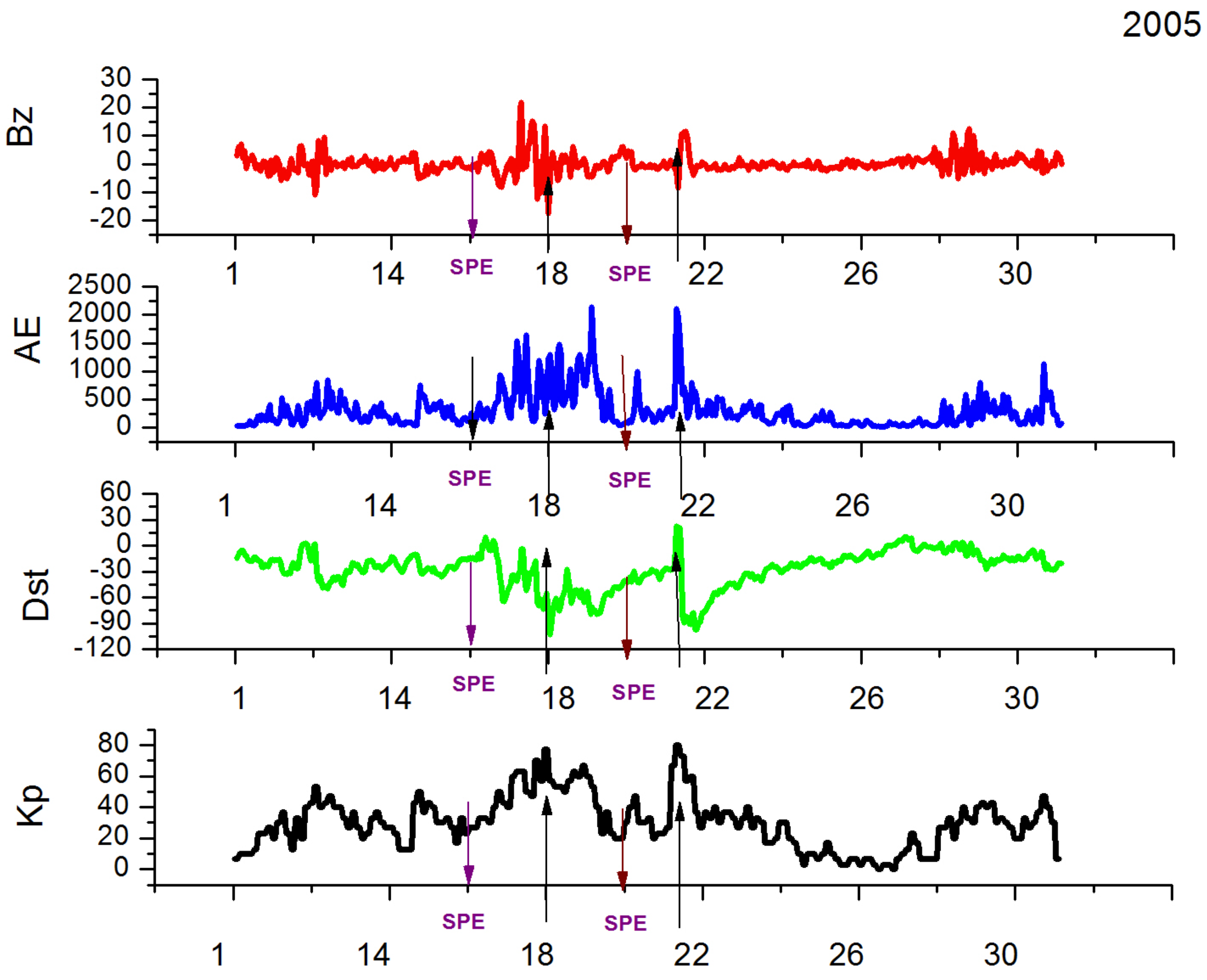
2. EPP During Solar Proton Events and Geomagnetic Disturbances in January of 2005 and 2012

EPPs are associated with fast, powerful energy-release phenomena, such as solar flares, coronal mass ejections, and geomagnetic disturbances. Precipitating solar protons, auroral, and radiation belt electrons are considered an important part of the natural forcing of the ionosphere and atmosphere.
Solar particle events, also known as solar proton events, occur when particles are emitted by the Sun, primarily protons accelerated either in the Sun’s atmosphere during a solar flare or in interplanetary space by the shock wave of a coronal mass ejection, penetrate the Earth’s magnetic field into the atmosphere, causing further ionization.
The NOAA Space Weather Prediction Center (SWPC) collects solar particle events regularly using data from geostationary GOES (Geosynchronous Operational Environmental Satellite) from 1976 till the present. The dataset includes proton flux information, which is a 5-minute average for energies more than 10 MeV, given in particle flux units (pfu or number of particles per cm 2 sr 1 s 1 ). Table 1 shows the NOAA SWPC collection of solar particle events (https://umbra.nascom.nasa.gov/SEP/, accessed on 20 January 2025) that took place in January of 2005 and 2012.
These four solar proton events (SPEs), see Table 1, can be ranked by their magnitude using the peak flux unit pfu. Virtually the same SPEs with energies more than 10 MeV are the SPE on 17 January 2005, with a proton flux of 5040 pfu, and the SPE on 24 January 2012, with a proton flux of 6310 pfu. A solar proton event on 28 January 2012 had a maximum magnitude peak flux of 796 pfu for energies greater than 10 MeV. On 20 January 2005, a solar proton event with an exceptionally hard spectrum was observed. This SPE was an event with the highest (more than 100 MeV) proton flux level observed since 1989 October (https://umbra.nascom.nasa.gov/SEP/, accessed on 20 January 2025). Energetic particles with energies below 500 MeV are well-measured onboard numerous spacecraft, but energetic particles with higher energies are detectable by ground-based neutron monitors [3,7,35]. Such types of solar proton events are named ground-level enhancement (GLE) events. Typically, solar proton events with a soft spectrum of energies more than 10 MeV play a major role in variations in the mesospheric chemical composition of the high-latitude ionosphere/atmosphere [2,3,16,28,32,36], while solar proton events of the GLE type with a harder spectrum do not have a significant effect on the chemistry of mesospheric altitudes [26,33].
The electron precipitation is strongly dependent on geomagnetic disturbances, although the relationship is complex. Many processes, such as the supply and accumulation of energy in the magnetosphere from the solar wind, the development of various waves, and the interaction of waves with particles, lead to the acceleration of electrons and their entry into the loss cone, which leads to the precipitation of energetic electrons into the Earth’s ionosphere/atmosphere. The strength of the geomagnetic field plays one of the main roles in the solar–Earth chain of relationships.
EPP intensity strongly depends on the north–south Bz component of the interplanetary magnetic field (IMF). The south direction of the Bz component of the IMF in near-Earth space determines intense geoeffective events connected with geomagnetic disturbances. Key criteria for intense geomagnetic disturbances are extended periods of the large southward Bz component of the IMF, which points opposite to the Earth’s magnetic field polarity. The largest southward Bz disturbances in the IMF lead to strong geomagnetic storms. Varying conditions in the solar wind cause changes in the structure of the magnetosphere and, accordingly, magnetospheric currents, which manifest themselves on the Earth’s surface as irregular geomagnetic variations. It is convenient to characterize magnetospheric dynamics, in general, by the level of these geomagnetic variations, in particular, by geomagnetic indices.
Geomagnetic indices describe variations in the Earth’s magnetic field caused by the impact of the solar wind on the Earth’s magnetosphere, as well as by changes within the magnetosphere, and the interaction of the magnetosphere and ionosphere. Geomagnetic disturbances are usually defined using various geomagnetic indices such as AE, Kp, Dst, etc. Different geomagnetic indices are usually defined at different latitudes, and each of the indices determines different current systems and associated precipitation of particles of a certain nature and different energies.
AE, the geomagnetic activity index characterizes magnetic disturbance in the polar auroral zone caused by the amplification of currents in the ionosphere flowing along the boundary of the auroral oval (eastern and western currents of the polar electrojet). The method for calculating AE is based on determining the magnitude of the deviation of the horizontal H component of the geomagnetic field from the quiet level. To calculate the AE index, geomagnetic data from 12 observatories located at auroral and subauroral latitudes and uniformly distributed over longitude are used. Increases in this index are mostly characterized by the precipitation of auroral electrons.
The Dst index of geomagnetic activity is obtained at low latitudes and characterizes the field change due to ring currents arising in the magnetosphere during geomagnetic storms. The influence of ring currents is reflected in a decrease in the horizontal H component of the geomagnetic field of the Earth with a maximum decrease at low latitudes. The Dst index is calculated as the average perturbation of the horizontal component of the Earth’s magnetic field intensity in an hourly interval, measured from a quiet level, determined using data from four low-latitude observatories uniformly distributed over longitude.
The Kp index is a planetary index characterizing the global disturbance of the Earth’s magnetic field in an hour time interval. The Kp index is defined as the average value of the disturbance levels of two horizontal components of the geomagnetic field observed at selected magnetic observatories located in the subauroral zone between about 50 and 60 degrees north and south geomagnetic latitudes.
Many data collections combine the variability of magnetospheric magnetic fields and geomagnetic indices that characterize geomagnetic disturbances. In our study, we used hourly AE and Dst indices obtained from the World Data Center for Geomagnetism, operated by the Data Analysis Center for Geomagnetism and Space Magnetism at Kyoto University. Kp*10 index and Bz component of the interplanetary magnetic field are obtained from the OMNI data sets.
Figure 1 and Figure 2 demonstrate temporal variations of the geomagnetic disturbances for January 2005 and January 2012. In these figures, the up arrows mark the starting points of the geomagnetic storm’s main phase, and the down arrows show the starting dates of solar proton events.
Figure 1 shows that on 16 January 2005, the IMF Bz component underwent strong variability, with the deepest negative value | B z | reaching 18 nT on 18 January 2005. The southward or negative value of the IMF Bz component largely determines the amount of energy and momentum transferred by the solar wind to the Earth’s magnetosphere, ionosphere, and atmosphere. That is clearly seen in the variability of geomagnetic indexes AE, Dst, and Kp; see Figure 1. On 18 January 2005, Dst decreased up to | D s t | = 103 nT, and Kp*10 reached 70. The maximum of the AE index up to 2136 nT was observed on 19 January 2005. It can be noted that the first disturbing geomagnetic period started from coronal mass ejection (CME) and solar flare class X2 at 23:02 UTC on 15 January. That led to a solar proton event started on 16 January at 02:10 UTC with a maximum proton flux of energies more than 10 MeV on 17 January at 17:50 UTC, see Table 1, and the disturbed geomagnetic activity started on 16 January 2005; see Figure 1. The second disturbing geomagnetic period started more suddenly with outstanding CME and solar flare class X7 on 20 January 2005 that stimulated the largest GLE in the last 50 years [35]. On 21 January 2005, the Bz component IMF decreased up to | B z | = 7 nT, the AE index increased up to 2111 nT, and Kp*10 reached 80. On 22 January 2005, Dst decreased up to | D s t | = 97 nT. The third disturbed geomagnetic period was less intense compared to the two previous and led to 163 standard substorms, with AE = 1130 nT and Kp*10 = 40.
Figure 2 shows temporal variations in the geomagnetic disturbances in January 2012. Moderate geomagnetic storms occurred on 21–25 January 2012. The geomagnetic disturbance period in January 2012 started from CME and solar flare class M2 on 19 January. IMF Bz is also consistent with the occurrence of CMEs. After the CME and magnetic clouds, the Bz component IMF sharply increased up to 20 nT and then strongly decreased to | B z | = 10 nT on 22 January 2012. Kp*10 reached 50, and on the next day, Dst decreased to | D s t | = 70 nT. AE increased to 1148 nT on 24 January 2012. Solar proton events were registered twice in January 2012, on 24 January 2012 at 15:30 UTC with maximum proton flux of energies more than 10 MeV 6310 pfu and on 28 January at 02:05 UTC with maximum proton flux of energies more than 10 MeV 796 pfu (Table 1).
Comparing Figure 1 and Figure 2 and the information from Table 1, we can conclude that stronger geomagnetic storms occurred during 16–23 January 2005 than during 21–25 January 2012; however, maximum proton fluxes of energies more than 10 MeV were observed during 23–24 January 2012 than during 16–17 January 2005. Both intervals had the same period of geomagnetic disturbances, and both took place in January.

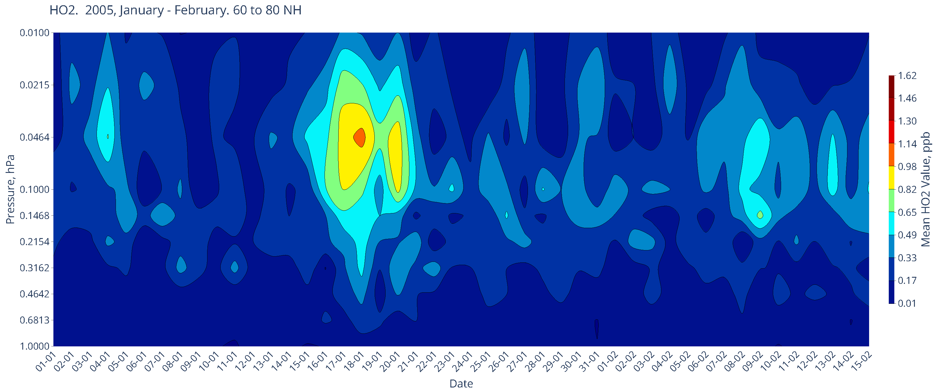
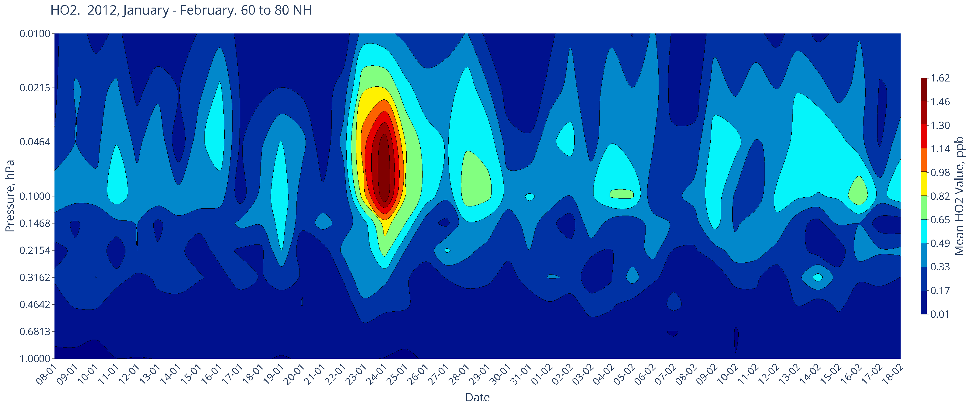
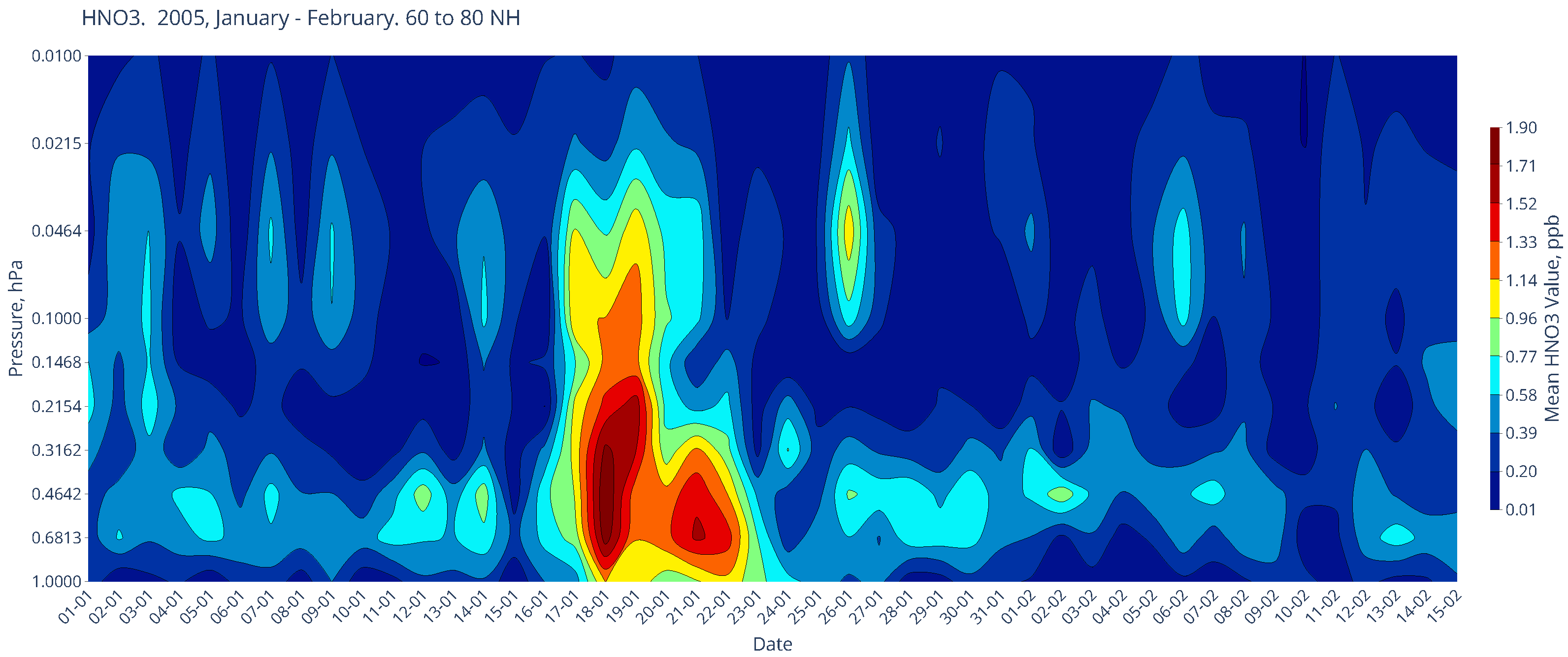
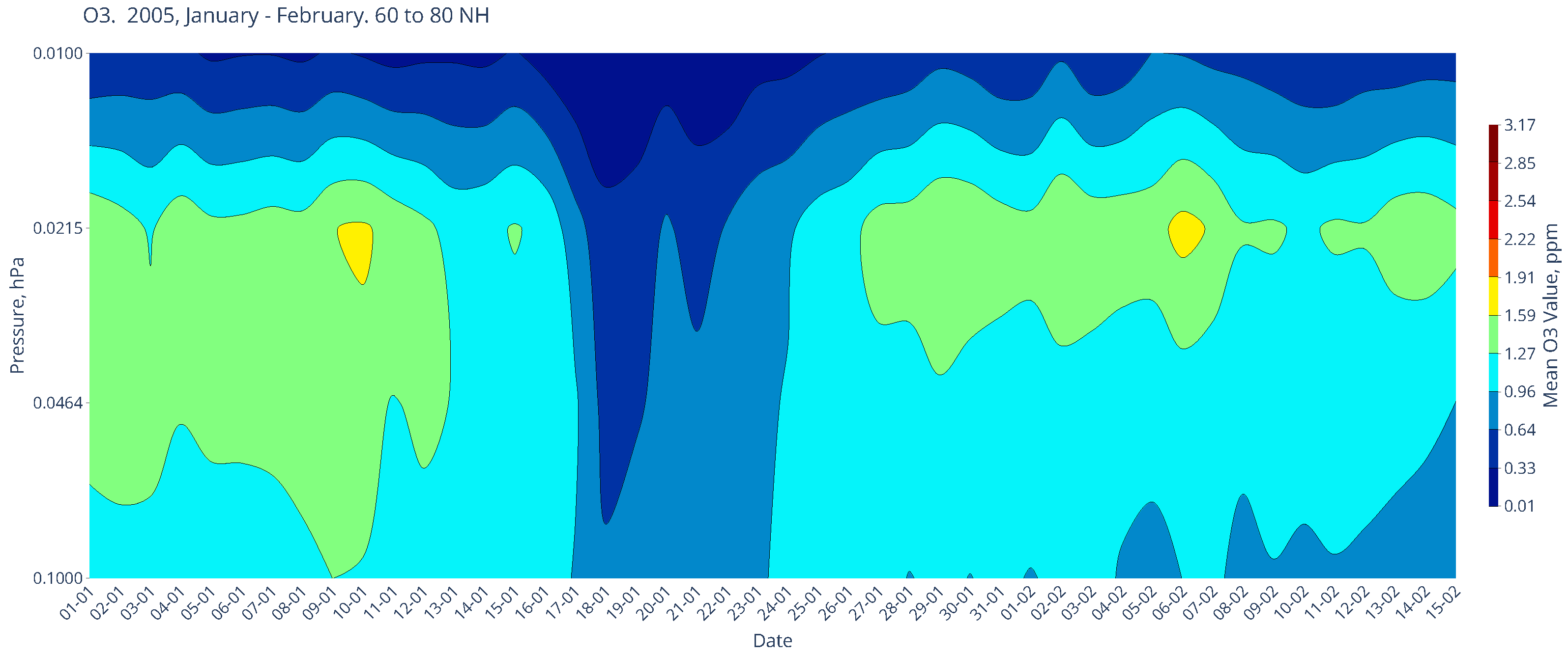
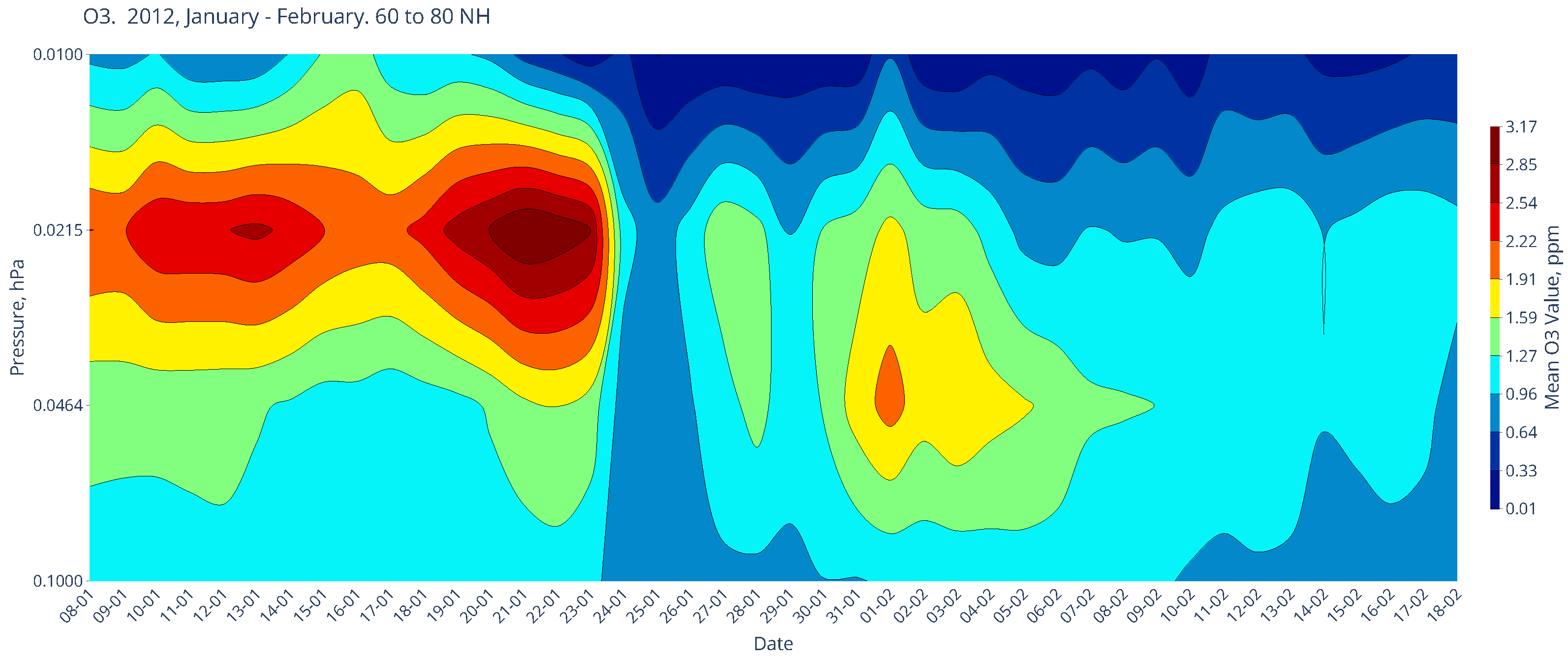
Chemical Composition in January of the Boreal Winters of 2005 and 2012

The Earth Observing System (EOS) Microwave Limb Sounder (MLS) is an instrument on NASA’s Aura spacecraft launched in July 2004. Aura is in a quasi-polar Sun-synchronous orbit at an altitude of 705 km. MLS registers millimeter and sub-millimeter wavelength thermal emissions, vertically scanning Earth’s limb in the orbit plane to give daily near-global coverage at about 80 NH to 80 NH latitude, with 15 orbits per day, making measurements during both day and night. Among the most interesting MLS/Aura retrieval products are H N O 3 , H O 2 , and ozone.
In our study, we consider the latest (version 5) MLS/Aura data with increased vertical range for ozone and some other species [37]. A new version of data retrieval has better quality in the upper mesosphere. Preliminary research has shown that the improvements are sufficient to increase the vertical range recommended for scientific use, for details, see https://mls.jpl.nasa.gov/data/v5-0_data_quality_document.pdf (accessed on 20 January 2025).
The response of the atmosphere to EPP depends on atmospheric conditions and availability of solar UV radiation that depends on the solar zenith angle [28,31,36]. In the absence of UV radiation, EPP plays an important role in the formations of the HO x and NO x families and leads to deeper ozone depletion in comparison to the periods when solar UV presents [28,31,36]. Although MLS/Aura provides chemical composition data for both hemispheres, we were unable to observe any significant response to EPP over the Southern Hemisphere in January 2005 and 2012. For this reason, we focus on the response in the northern mesosphere (the region from 0.01 hPa to 1 hPa, which is about 80–50 km) to the EPP observed in January 2005 and 2012. It is necessary to note that in the polar night mesosphere, primary increases in chemical compositions, like H N O 3 and H O 2 , can be induced only by EPP (electrons or protons) with electron energies that vary from tens of keV up to several MeV and with proton energies that vary from several MeV up to hundreds of MeV [3,38,39]. These particle energies can be observed during geomagnetic disturbances in January 2005 and 2012.
An increase in particle precipitation results in the production of H O x through complex positive ion chemistry [29]. The H O x produced by EPP is a direct function of ion pair production. In the mesosphere, H O x has a relatively short lifetime of several hours [3,29,40].
Figure 3 and Figure 4 demonstrate the altitudinal and temporal variability of H O 2 over 60 80 NH in January 2005 and 2012. In January 2005, a strong increase in H O 2 in the mesosphere started from 15 January 2005 and had a maximum enhancement around 0.046 hPa (about 70 km) after the onset of solar proton events; see Table 1. The second H O 2 maximum took place on 20 January 2005, on the day of the CME and GLE record; see Figure 3. Here, we can conclude that the maximum H O 2 production is strongly dependent on proton precipitation while the persistence of H O 2 in the mesosphere is connected with energetic electron precipitation that is strongly dependent on geomagnetic disturbances of the Earth’s magnetic field. It is explained by Figure 1 and Section 2, which illustrate strong geomagnetic storms that occurred 16–22 January 2005. In January 2012, a strong H O 2 increase in the mesosphere started from 22 January and reached maximum enhancement up to 1.62 ppb around 0.046 hPa (about 70 km) after the onset of solar proton events; see Figure 4. The second H O 2 maximum is associated with the SPE that began on January 27 and is less intense; see Figure 4. The first increase in H O 2 was due to a proton flux with a peak flux of up to 6310 pfu, and the second increase in H O 2 was due to a solar proton flux with a peak flux of 796 pfu; see Table 1. The comparison of Figure 3 and Figure 4 shows the maximum H O 2 enhancement of about 1.05 ppb and 1.62 ppb around 0.046 hPa (about 70 km) after the onset of solar proton precipitation in the second half of January 2005 and January 2012, respectively. The EPP-induced H O 2 enhancement is observed in the altitude range from 0.0215 hPa to 1 hPa over about 1 week; see Figure 3 and Figure 4.
The distribution of H N O 3 in polar night regions during the EPP is controlled by the ion chemistry, and the effects can cover the entire polar region [29,34,41,42]. Figure 5 and Figure 6 show altitudinal and temporal variability of H N O 3 over 60 80 NH in January 2005 and 2012. The EPP-induced increases of H N O 3 are observed between 0.0215 hPa and 1 hPa pressure levels over about 1 week. In January 2005, a strong increase of H N O 3 up to 1.9 ppb was noticeable near 0.46 hPa (about 50 km) after the onset of solar proton events on 17 January 2005; see Table 1. The second maximum of H N O 3 was observed near 0.6813 hPa after the GLE. Here, as in the case of H O 2 , the preservation of H N O 3 in the mesosphere is associated with the precipitation of energetic electrons, which strongly depends on geomagnetic disturbances of the Earth’s magnetic field; see Figure 1. Figure 6 shows the H N O 3 enhancement caused by EPP during the SPE on January 23, and the second, less intense H N O 3 increase is associated with the SPE on 27 January 2012. The comparison of Figure 3 and Figure 4 shows that the maximum H N O 3 enhancement is about 1.9 ppb and 1.66 ppb around 0.46 hPa (about 50 km) after the onset of solar proton precipitation in the second half of January 2005 and 2012, respectively.
The EPP-produced HO x is relatively short-lived (in our case HO 2 lived about a week) and leads to the destruction of mesospheric ozone. Figure 7 and Figure 8 illustrate the altitude and time variability of O 3 in the latitudinal range 60 80 NH in January 2005 and 2012. The O 3 depletion in January 2005 began on 17 January 250 and continued until 23 January 2005 in the height range of 0.01 hPa to 0.1 hPa (see Figure 7). At the same time, two peaks of ozone depletion were observed, one associated with the increase in HO 2 after the SPE on 17 January, and the second with the increase in HO 2 caused by the EPP on 20–21 January 2005. After 23 January 2005, O 3 content was completely recovered. Thus, it can be concluded that in January 2005, destruction of the ozone layer in the mesosphere after energetic particle precipitation and geomagnetic disturbances continued for about 1 week as the HO x components changed.
In January 2012, the situation with mesospheric O 3 destruction was quite different. MLS/Aura ozone observations show that O 3 volume mixing ratios were three times higher in January 2012 than in January 2005. Figure 8 shows the ozone loss starting from 23 January and associated with a CME and SPE; see Table 1. The second SPE in January 2012 started on 27 January and resulted in a weak H O x formation but did not result in mesospheric O 3 destruction. However, it is important to note that after 27 January, the MLS/Aura shows a small increase in O 3 and subsequent ozone destruction for about 1 month; see Figure 8. The comparison of Figure 7 and Figure 8 confirms that ozone recovery from EPP was much faster in January 2005 than in January 2012.

3. Summary and Conclusions

In this work, we analyzed observations of the Microwave Limb Sounder (MLS/Aura) measurements and found substantial enhancement of the hydroperoxyl radical HO 2 and nitric acid HNO 3 concentrations, as well as ozone depletion in the Northern Hemisphere (NH) polar night regions during energetic particle precipitation (EPP) in January of 2005 and 2012.
Strong EPP events with virtually the same proton flux were observed by GOES satellites in the second half of January 2005 and 2012. Geomagnetic disturbances in January 2005 were stronger, and Dst decreased to 103 nT compared to January 2012, when Dst decreased to 70 nT. In January 2005, the maximum Kp*10 reached 70, and in January 2012, the maximum Kp*10 reached 50. The strongest disturbances in the auroral zone were observed in January 2005, when the maximum AE index reached 2136 nT, while in January 2012, AE increased only to 1148 nT. It is clearly seen that stronger geomagnetic storms occurred in the period from 16 to 23 January 2005 than in the period from 21 to 25 January 2012; however, the maximum fluxes of protons with energies greater than 10 MeV were observed in the period from 23 to 28 January 2012 rather than in the period from 16 to 23 January 2005. On 20 January 2005, the strongest SPE/GLE event was recorded, and on 27 January 2012, another SPE was recorded, but it was less intense than the first. As a brief conclusion, we note that both considered periods took place in January, and both intervals are characterized by the same type of solar and geomagnetic disturbances.
According to MLS/Aura measurements, the volume mixing ratios of HO 2 and O 3 in January 2012 are higher than in January 2005. MLS/Aura data show that the highest HO 2 and HNO 3 mixing ratios, as well as the deepest ozone depletion, are observed in the 60 80 NH latitude range within the north polar vortex immediately after the maximum energetic particle flux recorded by GOES satellites in January 2025 and 2012. A second peak in HO 2 and HNO 3 mixing ratios was observed in January 2005, immediately after the GLE and increase in geomagnetic variability, but the second increase in HO 2 and HNO 3 in January 2012 is associated with weak SPE. The increase in HO 2 in the second half of January 2005 and January 2012 resulted in short-term mesospheric ozone depletion, as seen in the MLS/Aura ozone data. The maximum ozone depletion was around 0.02 hPa (about 75 km) due to the increase in HO x . Maximum O 3 destruction up to about 90% was observed on 18 January 2005 and 25 January 2012, respectively. The ozone recovery after the EPP was much faster in January 2005 than in January 2012.
Finally, it can be concluded that the loss of mesospheric ozone during the January energetic particle precipitation of the boreal winters of 2005 and 2012 was a consequence of successive solar proton events accompanied by disturbed geomagnetic activity. Apparently, two nearly simultaneous SPEs can lead to longer ozone depletion than a single SPE. However, the strength of the northern polar vortex can also play an important role in the duration of the ozone depletion period. Therefore, a strict understanding of what caused longer ozone destruction in January 2012 compared to 2005 requires additional research. Further chemistry–climate simulations are needed for understanding and explaining the huge difference in ozone depletion after virtually the same particle precipitation events observed in January 2005 and 2012.

Author Contributions

Conceptualization, I.M.; data analysis and results discussion, G.D., I.M. and E.R.; writing—original draft preparation, I.M., G.D. and E.R. All authors have read and agreed to the published version of the manuscript.

Funding

The work was supported by Saint Petersburg State University under research grant 116234986.

Institutional Review Board Statement

Not applicable.

Informed Consent Statement

Not applicable.

Data Availability Statement

NOAA SWPC SPE data: https://umbra.nascom.nasa.gov/SEP/ (accessed on 20 January 2025). Aura MLS data: https://mls.jpl.nasa.gov/ (accessed on 20 January 2025). World Data Center for Geomagnetism, Kyoto: https://wdc.kugi.kyoto-u.ac.jp/ (accessed on 20 January 2025). OMNI data: https://omniweb.gsfc.nasa.gov/html/ow_data.html (accessed on 20 January 2025). The data presented in this study are available on request from the corresponding authors.

Acknowledgments

The authors acknowledge all open datasets.

Conflicts of Interest

The authors declare no conflicts of interest.

References

  1. Randall, C.E.; Harvey, V.L.; Manney, G.L.; Orsolini, Y.; Codrescu, M.; Sioris, C.; Brohede, S.; Haley, C.S.; Gordley, L.L.; Zawodny, J.M.; et al. Stratospheric effects of energetic particle precipitation in 2003–2004. Geophys. Res. Lett. 2005, 32, L05802. [Google Scholar] [CrossRef]
  2. Rozanov, E.; Calisto, M.; Egorova, T.; Peter, T.; Schmutz, W. Influence of the Precipitating Energetic Particles on Atmospheric Chemistry and Climate. Surv. Geophys. 2012, 33, 483–501. [Google Scholar] [CrossRef]
  3. Mironova, I.A.; Aplin, K.L.; Arnold, F.; Bazilevskaya, G.A.; Harrison, R.G.; Krivolutsky, A.A.; Nicoll, K.A.; Rozanov, E.V.; Turunen, E.; Usoskin, I.G. Energetic Particle Influence on the Earth’s Atmosphere. Space Sci. Rev. 2015, 194, 1–96. [Google Scholar] [CrossRef]
  4. Matthes, K.; Funke, B.; Andersson, M.E.; Barnard, L.; Beer, J.; Charbonneau, P.; Clilverd, M.A.; Dudok de Wit, T.; Haberreiter, M.; Hendry, A.; et al. Solar forcing for CMIP6 (v3.2). Geosci. Model Dev. 2017, 10, 2247–2302. [Google Scholar] [CrossRef]
  5. Sinnhuber, M.; Berger, U.; Funke, B.; Nieder, H.; Reddmann, T.; Stiller, G.; Versick, S.; von Clarmann, T.; Maik Wissing, J. NOy production, ozone loss and changes in net radiative heating due to energetic particle precipitation in 2002–2010. Atmos. Chem. Phys. 2018, 18, 1115–1147. [Google Scholar] [CrossRef]
  6. Randall, C.; Harvey, L.; Pedatella, N.; Bailey, S.; Maruyama, N.; Chen, T. Sun-Earth Coupling via Energetic Particle Precipitation. Bull. Am. Astron. Soc. 2023, 55, 332. [Google Scholar] [CrossRef]
  7. Usoskin, I.G.; Kovaltsov, G.A.; Mironova, I.A. Cosmic ray induced ionization model CRAC:CRII: An extension to the upper atmosphere. J. Geophys. Res. 2010, 115, D10302. [Google Scholar] [CrossRef]
  8. Fang, X.; Randall, C.E.; Lummerzheim, D.; Wang, W.; Lu, G.; Solomon, S.C.; Frahm, R.A. Parameterization of monoenergetic electron impact ionization. Geoph. Res. Lett. 2010, 37, L22106. [Google Scholar] [CrossRef]
  9. Artamonov, A.A.; Mishev, A.L.; Usoskin, I.G. Atmospheric ionization induced by precipitating electrons: Comparison of CRAC:EPII model with a parametrization model. J. Atmos. Sol.-Terr. Phys. 2016, 149, 161–166. [Google Scholar] [CrossRef]
  10. Xu, W.; Marshall, R.A.; Tyssøy, H.N.; Fang, X. A Generalized Method for Calculating Atmospheric Ionization by Energetic Electron Precipitation. J. Geophys. Res. 2020, 125, e28482. [Google Scholar] [CrossRef]
  11. Mironova, I.; Kovaltsov, G.; Mishev, A.; Artamonov, A. Ionization in the Earth’s Atmosphere Due to Isotropic Energetic Electron Precipitation: Ion Production and Primary Electron Spectra. Remote Sens. 2021, 13, 4161. [Google Scholar] [CrossRef]
  12. Usoskin, I.G.; Kovaltsov, G.A.; Mishev, A.L. Updated model of cosmic-ray-induced ionization in the atmosphere (CRAC:CRII_v3): Improved yield function and lookup tables. J. Space Weather Space Clim. 2024, 14, 20. [Google Scholar] [CrossRef]
  13. Rycroft, M.J.; Nicoll, K.A.; Aplin, K.L.; Giles Harrison, R. Recent advances in global electric circuit coupling between the space environment and the troposphere. J. Atmos. Sol. Terr. Phys. 2012, 90, 198–211. [Google Scholar] [CrossRef]
  14. Bozóki, T.; Sátori, G.; Williams, E.; Mironova, I.; Steinbach, P.; Bland, E.C.; Koloskov, A.; Yampolski, Y.M.; Budanov, O.V.; Neska, M.; et al. Solar cycle-modulated deformation of the Earth-ionosphere cavity. Front. Earth Sci. 2021, 9, 735. [Google Scholar] [CrossRef]
  15. Kirillov, A.S. Calculation of rate coefficients of electron energy transfer processes for molecular nitrogen and molecular oxygen. Adv. Space Res. 2004, 33, 998–1004. [Google Scholar] [CrossRef]
  16. Jackman, C.H.; Marsh, D.R.; Vitt, F.M.; Garcia, R.R.; Fleming, E.L.; Labow, G.J.; Randall, C.E.; López-Puertas, M.; Funke, B.; von Clarmann, T.; et al. Short and medium term atmospheric constituent effects of very large solar proton events. Atmos. Chem. Phys. 2008, 8, 765–785. [Google Scholar] [CrossRef]
  17. Tacza, J.; Raulin, J.P.; Mendonca, R.R.S.; Makhmutov, V.S.; Marun, A.; Fernandez, G. Solar Effects on the Atmospheric Electric Field During 2010–2015 at Low Latitudes. J. Geophys. Res. 2018, 123, 11970–11979. [Google Scholar] [CrossRef]
  18. Meraner, K.; Schmidt, H. Climate impact of idealized winter polar mesospheric and stratospheric ozone losses as caused by energetic particle precipitation. Atmos. Chem. Phys. 2018, 18, 1079–1089. [Google Scholar] [CrossRef]
  19. Mishev, A.L. Application of the global neutron monitor network for assessment of spectra and anisotropy and the related terrestrial effects of strong SEPs. J. Atmos. Sol.-Terr. Phys. 2023, 243, 106021. [Google Scholar] [CrossRef]
  20. Georgieva, K.; Veretenenko, S. Solar influences on the Earth’s atmosphere: Solved and unsolved questions. Front. Astron. Space Sci. 2023, 10, 1244402. [Google Scholar] [CrossRef]
  21. Chum, J.; Langer, R.; Kolmašová, I.; Lhotka, O.; Rusz, J.; Strhárský, I. Solar cycle signatures in lightning activity. Atmos. Chem. Phys. 2024, 24, 9119–9130. [Google Scholar] [CrossRef]
  22. Siingh, D.; Singh, R.; Victor, N.J.; Kamra, A. The DC and AC global electric circuits and climate. Earth-Sci. Rev. 2023, 244, 104542. [Google Scholar] [CrossRef]
  23. Winant, A.; Pierrard, V.; Botek, E.; Herbst, K. The Atmospheric Influence on Cosmic-Ray-Induced Ionization and Absorbed Dose Rates. Universe 2023, 9, 502. [Google Scholar] [CrossRef]
  24. Funke, B.; Baumgaertner, A.; Calisto, M.; Egorova, T.; Jackman, C.H.; Kieser, J.; Krivolutsky, A.; López-Puertas, M.; Marsh, D.R.; Reddmann, T.; et al. Composition changes after the “Halloween” solar proton event: The High Energy Particle Precipitation in the Atmosphere (HEPPA) model versus MIPAS data intercomparison study. Atmos. Chem. Phys. 2011, 11, 9089–9139. [Google Scholar] [CrossRef]
  25. Andersson, M.E.; Verronen, P.T.; Marsh, D.R.; Seppälä, A.; Päivärinta, S.M.; Rodger, C.J.; Clilverd, M.A.; Kalakoski, N.; van de Kamp, M. Polar Ozone Response to Energetic Particle Precipitation Over Decadal Time Scales: The Role of Medium-Energy Electrons. J. Geophys. Res. 2018, 123, 607–622. [Google Scholar] [CrossRef]
  26. Mironova, I.; Karagodin-Doyennel, A.; Rozanov, E. The effect of Forbush decreases on the polar-night HOx concentration affecting stratospheric ozone. Front. Earth Sci. 2021, 8, 669. [Google Scholar] [CrossRef]
  27. Grankin, D.; Mironova, I.; Bazilevskaya, G.; Rozanov, E.; Egorova, T. Atmospheric Response to EEP during Geomagnetic Disturbances. Atmosphere 2023, 14, 273. [Google Scholar] [CrossRef]
  28. Doronin, G.; Mironova, I.; Bobrov, N.; Rozanov, E. Mesospheric Ozone Depletion during 2004–2024 as a Function of Solar Proton Events Intensity. Atmosphere 2024, 15, 944. [Google Scholar] [CrossRef]
  29. Solomon, S.; Rusch, D.W.; Gerard, J.C.; Reid, G.C.; Crutzen, P.J. The effect of particle precipitation events on the neutral and ion chemistry of the middle atmosphere: II. Odd hydrogen. Planet. Space Sci. 1981, 29, 885–893. [Google Scholar] [CrossRef]
  30. Porter, H.S.; Jackman, C.H.; Green, A.E.S. Efficiencies for production of atomic nitrogen and oxygen by relativistic proton impact in air. J. Chem. Phys. 1976, 65, 154–167. [Google Scholar] [CrossRef]
  31. Mironova, I.; Grankin, D.; Rozanov, E. Mesospheric Ozone Depletion Depending on Different Levels of Geomagnetic Disturbances and Seasons. Atmosphere 2023, 14, 1205. [Google Scholar] [CrossRef]
  32. Jackman, C.H.; Deland, M.T.; Labow, G.J.; Fleming, E.L.; Weisenstein, D.K.; Ko, M.K.W.; Sinnhuber, M.; Russell, J.M. Neutral atmospheric influences of the solar proton events in October-November 2003. J. Geophys. Res. 2005, 110, A09S27. [Google Scholar] [CrossRef]
  33. Jackman, C.H.; Marsh, D.R.; Vitt, F.M.; Roble, R.G.; Randall, C.E.; Bernath, P.F.; Funke, B.; López-Puertas, M.; Versick, S.; Stiller, G.P.; et al. Northern Hemisphere atmospheric influence of the solar proton events and ground level enhancement in January 2005. Atmos. Chem. Phys. 2011, 11, 6153–6166. [Google Scholar] [CrossRef]
  34. von Clarmann, T.; Funke, B.; López-Puertas, M.; Kellmann, S.; Linden, A.; Stiller, G.P.; Jackman, C.H.; Harvey, V.L. The solar proton events in 2012 as observed by MIPAS. Geophys. Res. Lett. 2013, 40, 2339–2343. [Google Scholar] [CrossRef]
  35. Usoskin, I.G.; Kovaltsov, G.A.; Mironova, I.A.; Tylka, A.J.; Dietrich, W.F. Ionization effect of solar particle GLE events in low and middle atmosphere. Atmos. Chem. Phys. 2011, 11, 1979–1988. [Google Scholar] [CrossRef]
  36. Jackman, C.H.; Randall, C.E.; Harvey, V.L.; Wang, S.; Fleming, E.L.; López-Puertas, M.; Funke, B.; Bernath, P.F. Middle atmospheric changes caused by the January and March 2012 solar proton events. Atmos. Chem. Phys. 2014, 14, 1025–1038. [Google Scholar] [CrossRef]
  37. Livesey, N.J.; Tang, A.J.; Chattopadhyay, G.; Stachnik, R.A.; Jarnot, R.; Kooi, J.W.; Millan, L.; Santee, M.L.; Chang, M.C.; Huang, R. A Continuity Microwave Limb Sounder (MLS) instrument to augment the record from Aura MLS. In Proceedings of the AGU Fall Meeting, Online, 1–20 December 2020; Volume 2020, p. A197-09. [Google Scholar]
  38. Turunen, E.; Verronen, P.T.; Seppälä, A.; Rodger, C.J.; Clilverd, M.A.; Tamminen, J.; Enell, C.F.; Ulich, T. Impact of different energies of precipitating particles on NOx generation in the middle and upper atmosphere during geomagnetic storms. J. Atmos. Sol.-Terr. Phys. 2009, 71, 1176–1189. [Google Scholar] [CrossRef]
  39. Artamonov, A.; Mironova, I.; Kovaltsov, G.; Mishev, A.; Plotnikov, E.; Konstantinova, N. Calculation of atmospheric ionization induced by electrons with non-vertical precipitation: Updated model CRAC-EPII. Adv. Space Res. 2017, 59, 2295–2300. [Google Scholar] [CrossRef]
  40. Sinnhuber, M.; Nieder, H.; Wieters, N. Energetic Particle Precipitation and the Chemistry of the Mesosphere/Lower Thermosphere. Surv. Geophys. 2012, 33, 1281–1334. [Google Scholar] [CrossRef]
  41. Orsolini, Y.J.; Urban, J.; Murtagh, D.P. Nitric acid in the stratosphere based on Odin observations from 2001 to 2009–Part 2: High-altitude polar enhancements. Atmos. Chem. Phys. 2009, 9, 7045–7052. [Google Scholar] [CrossRef]
  42. Verronen, P.T.; Santee, M.L.; Manney, G.L.; Lehmann, R.; Salmi, S.M.; Seppälä, A. Nitric acid enhancements in the mesosphere during the January 2005 and December 2006 solar proton events. J. Geophys. Res. 2011, 116. [Google Scholar] [CrossRef]
Figure 1. The temporal variations in the north–south Bz (nT) component of the interplanetary magnetic field, Dst (nT) index, AE (nT) index, and Kp*10 index in January 2005. Up arrows mark starting points of the main phase of geomagnetic storms. Down arrows show the starting dates of solar proton events. Red line—temporal variability of the IMF Bz component. Blue line—temporal variability of AE (nT) index. Green line—temporal variability of Dst (nT) index. Black line—temporal variability of Kp*10 index.
Atmosphere 16 00506 g001
Figure 2. The temporal variations of the north–south Bz (nT) component of the interplanetary magnetic field, Dst (nT) index, AE (nT) index, and Kp*10 index during January 2012. Up arrows mark starting points of the main phase of geomagnetic storms. Down arrows show the starting dates of solar proton events. Red line—temporal variability of the IMF Bz component. Blue line—temporal variability of AE (nT) index. Green line—temporal variability of Dst (nT) index. Black line—temporal variability of Kp*10 index.
Atmosphere 16 00506 g002
Figure 3. Altitudinal and temporal variability of HO 2 over Northern Polar Hemisphere 60 80 NH in January 2005.
Atmosphere 16 00506 g003
Figure 4. Altitudinal and temporal variability of HO 2 over Northern Polar Hemisphere 60 80 NH in January 2012.
Atmosphere 16 00506 g004
Figure 5. Altitudinal and temporal variability of HNO 3 over Northern Polar Hemisphere 60 80 NH in January 2005.
Atmosphere 16 00506 g005
Figure 6. Altitudinal and temporal variability of HNO 3 over Northern Polar Hemisphere 60 80 NH in January 2012.
Atmosphere 16 00506 g006
Figure 7. Altitudinal and temporal variability of O 3 over Northern Polar Hemisphere 60 80 NH in January 2005.
Atmosphere 16 00506 g007
Figure 8. Altitudinal and temporal variability of O 3 over Northern Polar Hemisphere 60 80 NH in January 2012.
Atmosphere 16 00506 g008
Table 1. Solar proton events (SPEs) in January of 2005 and January of 2012.
SPE Start DateSPE Maximum Date>10 MeV Maximum (pfu)
D M Yr (UTC) Yr M/D (UTC)
16 January 2005 (02:10)17 January 2005 (17:50)5040
20 January 2005 (—)20 January 2005 (08:10)1860
23 January 2012 (05:30)24 January 2012 (15:30)6310
27 January 2012 (19:05)28 January 2012 (02:05)796
Disclaimer/Publisher’s Note: The statements, opinions and data contained in all publications are solely those of the individual author(s) and contributor(s) and not of MDPI and/or the editor(s). MDPI and/or the editor(s) disclaim responsibility for any injury to people or property resulting from any ideas, methods, instructions or products referred to in the content.

