Abstract
PM2.5 levels increase in cities during the first hours of the year due to combustion activities and the use of fireworks. In Quito (2800 masl), the capital of Ecuador, air quality records at the beginning of 2020 to 2025 (6 years) ranged between 13.4 and 217.8 µg m−3 (maximum mean levels for 24 h), most of them being higher than 15.0 µg m−3, the current recommended concentration by the World Health Organization (WHO), highlighting the need to decrease these emissions and promote actions to reduce the exposure to these extreme events. Air pollution forecasting as a preventive warning system could help achieve this objective. Therefore, the primary aim of this research was to analyze the variation in PM2.5 levels in this city during the initial hours of the year to define, through numerical experiments, the spatiotemporal configuration of PM2.5 emissions to reproduce the observed PM2.5 levels and obtain insights to build an emission-based forecasting tool. For this purpose, we modeled atmospheric variables and the PM2.5 levels using the Weather Research and Forecasting with Chemistry (WRF-Chem) model. Consistent with the behavior suggested by records of associated meteorological variables, the modeled planetary boundary layer height (PBLH) was generally lower in the city’s south compared with the center and the north. The records and modeled results indicated that in the south, the higher PM2.5 levels were produced by higher emissions and lower values of the PBLH compared with the center and north, highlighting the importance of reducing the PM2.5 emissions. The emission maps used for modeling the dispersion at the beginning of 2024 and 2025 are proposed as inputs for the future forecasting of the PM2.5 levels at the start of the year, as preventive information for the public, to discourage, in advance, both combustion activities and the use of fireworks and to take action to avoid exposure.
1. Introduction
By midnight on 31 December in Ecuador, in a festive environment, it is a tradition to burn “años viejos”, which are cloth dolls filled with sawdust and paper, and fireworks. This celebration is considered a sociocultural expression rooted in the lives of Ecuadorians, as a fire ritual for the culmination of one cycle and the birth of another. The people express their intention to leave behind the negative moments and sustain themselves in the hope of a more propitious and favorable new year [1].
However, this practice is accompanied by air pollution [2], noise, and other environmental concerns [3]. Due to the combustion activities and burning of fireworks, as in different parts of the world [2,4], the PM2.5 levels in the atmosphere typically reach concentrations higher than 15 µg m−3 (maximum mean levels for 24 h), the current concentration recommended by the World Health Organization (WHO) for short-term exposure [5]. Usually, at the beginning of the year, the PM2.5 concentrations in Quito (2800 masl) and Cuenca (2550 masl), the two Ecuadorian Andean cities currently operating air quality networks in the country, are the highest of the year [6,7].
Short-term PM2.5 pollution caused by these practices affects public health, promoting asthma attacks, lung infections, eye allergies, cough, cardiovascular disease, and respiratory mortality, while also reducing visibility [2,8,9,10]. Most particles aerosolized by burning fireworks are metals, including lead, nickel, antimony, barium, magnesium, and iron, which are used to create the vibrant colors of fireworks [4,11,12]. These metals can have adverse effects on mammalian cells and the lungs [12], as well as on the quality of water bodies [13]. The fireworks’ smoke is especially hazardous to children, older adults, pregnant women, and individuals with lung or heart disease [14].
Different studies have reported air quality levels resulting from the use of fireworks. Singh et al. (2019) reviewed their role in air quality, visibility, and human health, reporting exceptional short-term high levels of pollution in different parts of the world, with peak concentrations exceeding ambient levels by 2–8 times, and decreases of up to 92% in visibility [8], although returning to normal air quality levels, typically within 24 h after such events. Zhang et al. (2020) reported the effects of fireworks during the Chinese Lunar New Year celebrations, with remarkable increases in nationwide PM2.5 concentrations, which were 159~223% higher than the average level [15]. Manchanda et al. (2022) analyzed the chemical composition of PM2.5 during the Diwali Indian festival, reporting that PM2.5 concentrations were up to 16 times higher than pre-firework levels, while the elemental, organic, and black carbon fractions increased by factors of 46.1, 3.7, and 5.6, respectively [16]. Mousavi et al. (2021) analyzed the impact of the 4th of July (2019 and 2020) fireworks on levels in California (United States), identifying correlations between PM2.5 measurements and socioeconomic status (SES) and reporting that peaks were over two times higher among communities with a lower SES [10].
Long-term exposure to particulate matter and outdoor air pollution is carcinogenic to humans [17,18]. The mean annual levels of PM2.5 in Quito and Cuenca reached values between 17.3 and 19.8 µg m−3 [19], and 6 and 14 µg m−3 [7], respectively, which exceed the current WHO guideline of 5 µg m−3 [5].
Air pollution levels result from the interaction between emissions and atmospheric conditions [20,21]. The planetary boundary layer height (PBLH), the turbulent bottom component of the atmosphere, shows a daily cycle of depth, being lowest at sunrise and highest a couple of hours after midday [22]. The PBLH acts as an upper boundary and defines the volume of the atmosphere in which air pollutants can disperse.
Different options, such as controlling both combustion activities and the use of fireworks, can be explored to decrease the levels of PM2.5 at the beginning of the year. Another could be advancing the time for PM2.5 emissions to when the PBLH is higher than at midnight and, therefore, there are better atmospheric conditions to disperse the air pollutants. Numerical experiments in Cuenca studied the last option through a pioneering research activity in Ecuador [23].
Air pollution forecasting, as preventive warning information [24,25,26,27], is another way to help reduce exposure to PM2.5. It is connected to several of the Sustainable Development Goals (SDGs), including good health and well-being (SDG 3) and sustainable cities and communities (SDG 11) [28]. When people have access to air quality forecasts, they should adjust their activities and behaviors to minimize or avoid exposure.
Quito (longitude −78.5, latitude −0.2), Ecuador’s capital, is located near the Equator (Figure 1). Due to its high altitude above sea level, any combustion activity produces more primary emissions due to the lower availability of oxygen. Therefore, the primary objective of this research was to analyze the variation in PM2.5 levels in this city during the initial hours of the year in order to define the spatiotemporal configuration of PM2.5 emissions to operate an emission-based air pollution forecasting tool. For this purpose, in this manuscript, the following questions are addressed:
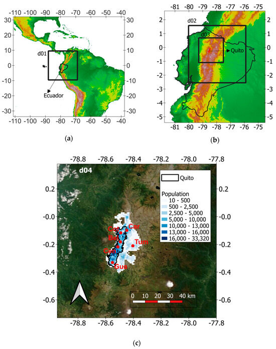
Figure 1.
(a) Location of Ecuador. (b) Location of Quito. (c) The urban area of Quito (black border). The red dots in (c) indicate the locations of the air quality stations: Car, Carapungo; Cot, Cotocollao; Bel, Belisario; Cen, Centro; Gua, Guamaní; Tum, Tumbaco. The blue colors in (c) depict the population distribution. Domains for modeling the dispersion of PM2.5: d01 ((a) master domain), d02 ((b) first subdomain), d03 ((c) second subdomain), and d04 ((c) third subdomain). Geographical coordinates are indicated in degrees.
- What were the PM2.5 levels at the beginning of recent years, and what can explain them?
- What was the magnitude of the PM2.5 emissions?
- What are the magnitude and spatiotemporal configuration of PM2.5 emissions that can be used for forecasting purposes?
To address these questions, we analyzed the atmospheric records and modeled the weather in Quito. Additionally, through numerical experiments using a state-of-the-art air quality model, we created PM2.5 emission maps, which were used to study the dispersion of PM2.5 at the beginning of the selected years.
2. Methods
2.1. The Air Quality Network
According to national regulatory requirements, the air quality network in Quito has been operational since 2004, providing reliable records of air pollution and meteorological variables at the surface, initially with eight automatic stations [6]. For this manuscript, and based on the availability of records, the data from six stations were used (Figure 1): two located in the north (Carapungo, Car; Cotocollao, Cot), and one in the center-north (Belisario, Bel), in the historic center (Centro, Cen), in the south (Guamaní, Gua), and in the Tumbaco Valley (Tumbaco, Tum).
The records from the historic center of Quito (Cen station) from 2005 to 2023 were processed to obtain the annual mean levels of PM2.5, which ranged between 12.8 and 21.5 µg m−3, all of which were higher than the current WHO guideline for long-term exposure (5 µg m−3) [15]. The lowest value corresponded to 2020, when the lockdown due to the COVID-19 pandemic occurred [29]. The highest concentration occurred in 2007 and subsequently decreased, reaching 15.1 µg m−3 in 2023. From 2005 to 2023, on 62.3% of the days, the mean daily PM2.5 levels exceeded the current WHO guideline for short-term exposure (15 µg m−3).
Focusing on the effects of combustion activities at the beginning of the year, from 2020 to 2025 (6 years), the records from the six stations (maximum mean levels for 24 h; 36 records) indicated that the PM2.5 levels ranged between 13.4 and 217.8 µg m−3, and most of them (93.3%) were higher than 15.0 µg m−3 (Figure 2). The highest records were measured at the Gua station, located south of the city, with levels ranging from 34.7 to 217.8 µg m−3. The lowest and highest concentrations were recorded at the beginning of 2025 and 2024, respectively. These concentrations were 2.3 and 14.5 times higher than the WHO’s guideline for long-term exposure, respectively.
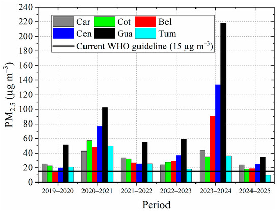
Figure 2.
PM2.5 records (maximum mean for 24 h) in Quito at the beginning of the selected years.
Figure 3 depicts the hourly PM2.5 records during 31 December and 1 January. At the Gua station (south of Quito), the maximum hourly records ranged from 200.9 µg m−3 on 1 January 2025 to 745.9 µg m−3 on 1 January 2024.
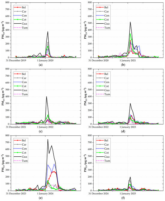
Figure 3.
Hourly PM2.5 records during 31 December and 1 January: (a) 2019–2020. (b) 2020–2021. (c) 2021–2022. (d) 2022–2023. (e) 2023–2024. (f) 2024–2025.
2.2. Meteorological Data
From the meteorological variables measured at the stations, temperature and wind speed were selected to explore their behaviors as parameters directly involved in the atmosphere’s stability [22] and, therefore, in its capacity to disperse or prevent the dispersion of air pollutants. The hourly records of these variables on 31 December and 1 January 1 were analyzed.
2.3. Weather Modeling
To gain insights into the influence of meteorological variables in the dispersion of PM2.5, the weather on 31 December and 1 January was simulated using the Weather Research and Forecasting (WRF V4.4) model, based on the selection of parameters recommended from atmospheric (meteorology and air pollution) modeling studies in Cuenca [30], a city with similar features to Quito in terms of their complex topographies, their heights above sea level, and the complexity of the land categories. WRF is a state-of-the-art numerical Eulerian 3D weather model used for research and forecasting from regional to global scales [31].
We used four domains for modeling (Figure 1): the master grid (d01, 80 × 80 cells, 27 km on each side), covering the north-western region of South America; the first subdomain (d02, 52 × 52 cells, 9 km on each side), covering the upper half of Ecuador; the second subdomain (d02, 67 × 67 cells, 3 km on each side), involving the Metropolitan Area of Quito territory; and the third and inner subdomain (d04, 121 × 121 cells, 1 km on each side), covering the urban area of Quito (Figure 1c). The atmospheric dataset of the Global Operational Analysis (Final, FNL) was selected to generate the initial and boundary conditions [32]. Table 1 indicates the main choices.

Table 1.
Schemes and options selected for atmospheric modeling in Quito [33].
2.4. PM2.5 Emission Modeling
We began estimating the emission of PM2.5 due to the combustion and use of fireworks at the beginning of the year. For this purpose, we first created a population map by processing the geographical data on Quito’s population density for 2019 [40]. The spatial distribution of the population was managed with a geographical information tool to map the population to the cells of the d04 domain (Figure 1c).
Using a reference emission factor, options for the spatial configuration of the emissions for two scenarios were explored: the first, a PM2.5 emission map to numerically reproduce the dispersion of the very high levels recorded at the beginning of 2024, and the second, a PM2.5 emission map to recreate the high levels recorded at the beginning of 2025. In each cell of d04, the basic emission model was applied (Equation (1)):
Ei: PM2.5 emissions in cell i (i = 1 to 14,400);
Pi: population in cell i;
EF: reference emission factor (2.7 g PM2.5 person−1);
Fi: factor applied in cell i.
A reference emission factor of 2.7 g PM2.5 per person was deduced for Cuenca by modeling the effects on PM2.5 levels of advancing the time of combustion activities at the beginning of the year [23]. This emission factor included the contributions from the combustion of puppets and the use of fireworks.
To generate the hourly PM2.5 emissions, the total emission in each cell (Ei) was distributed using factors of 20%, 15%, 15%, 15%, 10%, and 10% for the period from 01:00 LT to 07:00 LT on 1 January, respectively. As PM2.5 background emissions on 31 December and 1 January, the contribution from on-road traffic during holidays was considered [41,42].
2.5. PM2.5 Dispersion Modeling
To infer the configuration of the emissions maps for the two scenarios, different versions of the PM2.5 emission maps were built. They were used to simulate the dispersion in d04, using the Weather Research and Forecasting with Chemistry model (WRF-Chem V3.2). It is an extension of the WRF model that simultaneously reads emission data and models meteorological variables and air pollutant dispersion. For the chemistry option, the GOCART simple aerosol scheme (CHEM_OPT = 300) was selected, which has no ozone chemistry and does not include direct or indirect effects between aerosols and meteorology.
2.6. Metrics for Modeling Performance
The following metrics were used to assess the modeling performance of temperature [43]:
GE: gross error, n: number of records, Pi: predicted value, and Oi: observed value.
B: bias, Pm: mean predicted value, and Om: mean observed value.
IOA: index of agreement.
To assess the modeling performance of wind speed, the root-mean-square error (RMSE) and B (bias, Equation (3)) were applied:
In addition, the percentages of meteorological records captured by modeling were computed based on the desired accuracies specified in Table 2, which are suggested for applying models under the European Union’s Air Quality Directive [43]. For PM2.5 levels (mean value over 24 h), we considered the model to have properly captured the corresponding record if the difference was less than 50%.
Table 2.
Metrics for modeling atmospheric variables [43].
3. Results and Discussion
3.1. Meteorology
Figure 4 illustrates the hourly temperature records for 31 December and 1 January. They indicated that the lowest temperatures were measured at the Gua station. At 01:00 on 1 January, this station’s temperature ranged between 8.8 and 11.3 °C. The temperatures at the Car, Cot, Bel, and Cen stations ranged between 10.1 and 13.3 °C. The meteorological records of the air quality network from Quito indicate that, over the last six years (2000–2025), the city’s south experienced lower temperatures than the center and north.
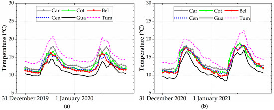
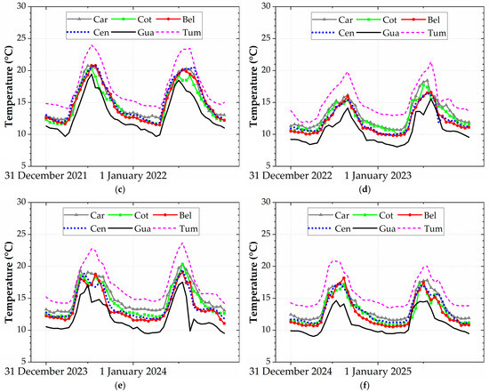
Figure 4.
Hourly temperature records during 31 December and 1 January: (a) 2019–2020. (b) 2020–2021. (c) 2021–2022. (d) 2022–2023. (e) 2023–2024. (f) 2024–2025.
The WRF model captured the surface temperature behavior (Figure 5; Table 3). For most periods and stations, the values of the GE and B were in the benchmark ranges. The IOA was higher than 0.8 for all cases, indicating a strong relationship between the measured and modeled temperatures. The percentage of the surface temperature captured by modeling ranged from 60.4% to 97.8% (Table 4), with a median value of 83.3%.
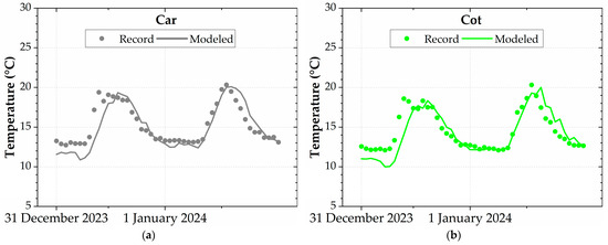
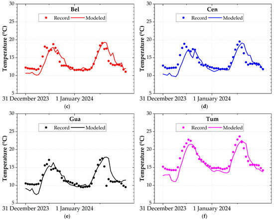
Figure 5.
Observed versus modeled temperatures during 31 December 2023 and 1 January 2024: (a) Car; (b) Cot; (c) Bel; (d) Cent; (e) Gua; (f) Tum.
Table 3.
Metrics for modeling surface temperature. Bold numbers highlight the values fitting the benchmark.
Table 4.
Percentages of capturing surface temperature by modeling. Bold numbers highlight the values more significant than 70%.
For the five stations in the urban area of Quito (Car, Cot, Bel, Cen, and Gua), the WRF model obtained RMSE values in the benchmark range for modeling wind speed (Table 5). However, the MB values were positive and higher than the benchmark upper limit. The percentage of wind speed captured by modeling ranged from 43.8% to 77.1% (Table 6), with a median value of 59.4%. The modeled wind speed values were higher than records at midday and the first hours of the afternoon. They were consistent with the records during the night and the first hours of the morning, when the PM2.5 emissions from combustion and fireworks occurred.
Table 5.
Metrics for modeling wind speed. Bold numbers highlight the values fitting the benchmark.
Table 6.
Percentages of capturing wind speed by modeling. Bold numbers highlight the values more significant than 60%.
Modeling accurately captured the surface temperature and wind speed, two atmospheric variables linked to atmospheric stability, implying that the PBLH was also accurately captured by the modeling.
Figure 6 depicts the modeled temperature maps on 1 January at 01:00 (LT). The Car station showed mostly temperatures between 12 and 15 °C. The Cot, Bel, and Cen stations mainly showed values between 10 and 12 °C. According to the records, the model consistently computed lower temperatures for the Gua station, with values ranging between 5 and 10 °C. Figure 7 depicts the modeled PBLH maps on 1 January at 01:00 (LT). The Car, Cot, Bel, and Cen stations mainly showed values between 90 and 400 m. At Gua station, the computed PBLH was primarily lower than 90 m.
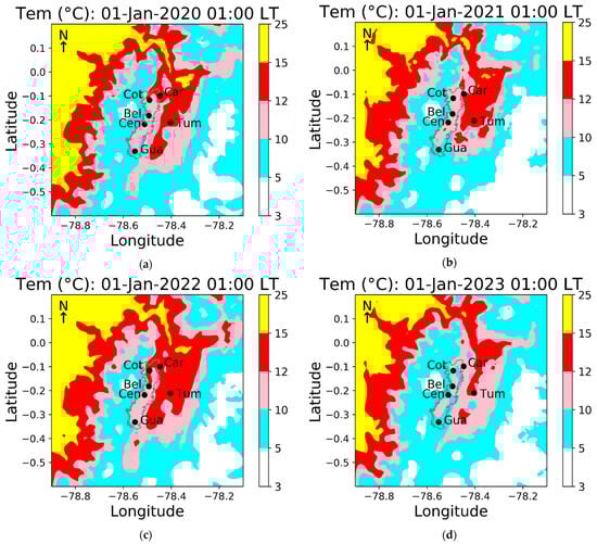
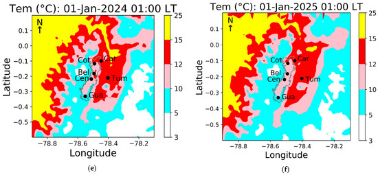
Figure 6.
Modeled temperatures on 1 January at 01:00 AM (LT): (a) 2020; (b) 2021; (c) 2022; (d) 2023; (e) 2024; (f) 2025. Geographical coordinates are indicated in degrees.

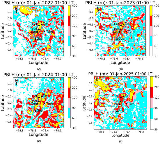
Figure 7.
Modeled planetary boundary layer height (PBLH) values on 1 January at 01:00 AM (LT): (a) 2020; (b) 2021; (c) 2022; (d) 2023; (e) 2024; (f) 2025. Geographical coordinates are indicated in degrees.
Numerical modeling consistently showed a lower temperature in the city’s south, which resulted in a lower PBLH compared with the center and north of Quito. This suggested a reduced capacity to disperse PM2.5 emissions in southern Quito, exacerbating the effects of combustion activities and fireworks at the beginning of the year.
3.2. PM2.5 Emissions and Dispersion Modeling
Initially, we created the first version of the PM2.5 emission maps for each scenario, using a value of 1 for the Fi parameter (Equation (1)) in all cells of d04. However, the modeled PM2.5 results were not consistent with the records. Therefore, various options for Fi were explored. After testing a range of configurations, we identified a suitable version for each scenario, which produced consistent computed PM2.5 concentrations compared with the records. The final version of the PM2.5 emission maps required values of the Fi parameter to range between 0.3 and 12 for 1 January 2024 and between 0.9 and 2.7 for 1 January 2025.
Figure 8 illustrates the spatial distribution of the PM2.5 emissions resulting from combustion activities and fireworks at the beginning of 2024 and 2025, totaling 10.1 and 11.2 t, respectively. On 1 January 2024, the cells with the highest emissions were located south of the city. On 1 January 2025, the highest emissions were located in the cells over the south and center. Although the total PM2.5 emissions were of a similar magnitude, the spatial configuration was particular for each scenario.
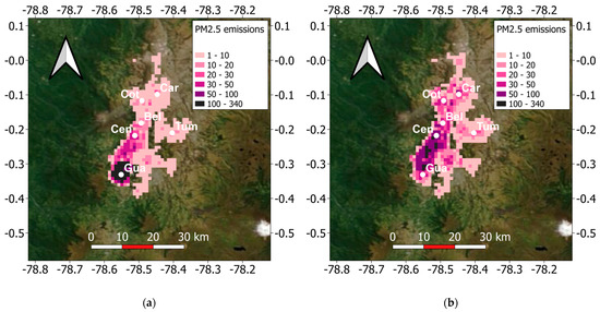
Figure 8.
PM2.5 emissions due to combustion and the use of fireworks at the beginning of 2024 (a) and 2025 (b). Geographical coordinates are indicated in degrees.
The PM2.5 emissions from on-road traffic in Quito for the year 2012 were estimated at 1211.2 t y−1 [42]. As a first reference, the percentage of PM2.5 emissions at the beginning of the year due to combustion activities and fireworks compared with the on-road traffic contribution ranged between 0.83% and 0.92%. For Cuenca, this percentage was 0.32%, considering the PM2.5 emission at the beginning of 2021 (1.73 t y−1) and the on-road traffic contribution for the same year 2021 (534.3 t y−1) [44,45].
Figure 9a–f illustrates the hourly PM2.5 levels of recorded data and modeled PM2.5 values from 31 December 2023 to 1 January 2024. The pattern of the modeled levels was consistent with the records at the six stations. The linear correlation between the PM2.5 (maximum mean over 24 h) records and the modeled values yielded a Pearson’s coefficient (r) of 0.98 (Figure 9g), comparable to the performance (r = 0.94) when modeling the dispersion of PM2.5 in Cuenca at the beginning of 2022 [23]. The records at the six stations were captured by modeling.
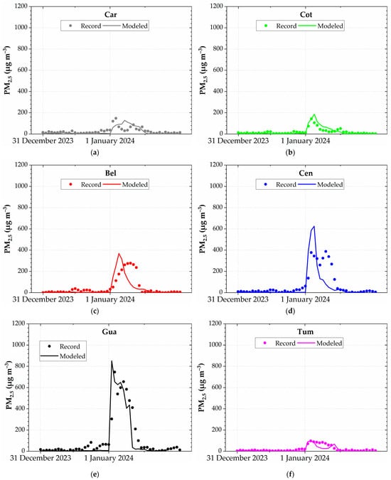
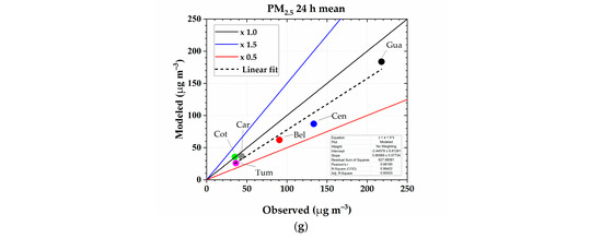
Figure 9.
Observed and modeled hourly PM2.5 levels: (a) Cot, (b) Car, (c) Bel, (d) Cen, (e) Gua, and (f) Tum. (g) Comparison of observed and modeled PM2.5 levels (maximum mean for 24 h) on 1 January 2024.
The modeled results indicated that part of the emissions from the south were transported toward the northeast and north of the city. Some of the emissions were also directed westward from the south and the center of Quito (Figure 10). The modeled peak hourly concentrations reached levels between 800 and 1100 µg m−3 in the southern part of the city. The highest PM2.5 modeled values (maximum mean over 24 h) occurred in the center and south of the city, with levels ranging from 80 to 240 µg m−3 (Figure 10).
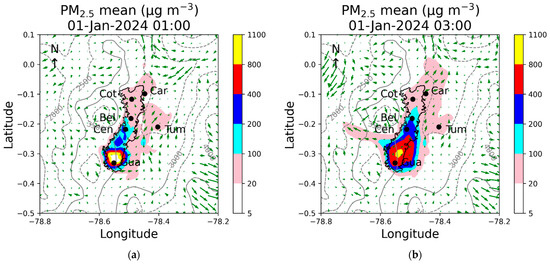
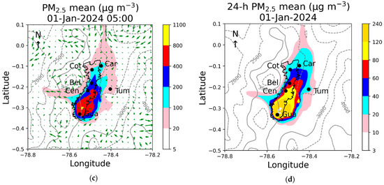
Figure 10.
Modeled PM2.5 levels for 1 January 2024: (a) 01:00, (b) 03:00, (c) 05:00, and (d) PM2.5 levels on 1 January 2024 (maximum mean for 24 h). The grey lines indicate topography. Geographical coordinates are indicated in degrees.
Figure 11 depicts the hourly PM2.5 levels of records and modeled PM2.5 values from 31 December 2024 to 1 January 2025. Similarly, the pattern of the modeled levels was consistent with the records at the six stations. The linear correlation between the PM2.5 (mean during 24 h) records and the modeled values obtained a Pearson’s coefficient (r) of 0.94 (Figure 11g).
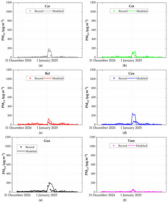
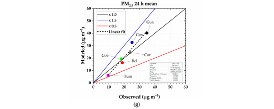
Figure 11.
Observed and modeled hourly PM2.5 levels: (a) Cot, (b) Car, (c) Bel, (d) Cen, (e) Gua, and (f) Tum. (g) Comparison of observed and modeled PM2.5 levels (maximum mean for 24 h) on 1 January 2025.
The modeled results highlight a complex wind configuration (Figure 12). Over the upper half of the city, the wind came from the north and northeast. Over the lower half, the wind coming from the west transported part of the emissions toward the east of this part of the city. The modeled peak hourly concentrations reached levels between 100 and 400 µg m−3 between the Gua and Cen stations. Over the urban area of Quito, the highest PM2.5 modeled levels (maximum mean over 24 h) occurred in the vicinity of these stations, with levels ranging from 40 to 60 µg m−3 (Figure 12).
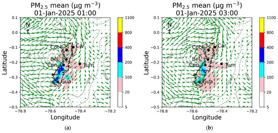
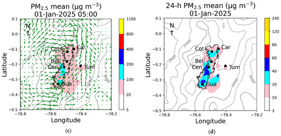
Figure 12.
Modeled PM2.5 levels for 1 January 2025: (a) 01:00, (b) 03:00, (c) 05:00, and (d) PM2.5 levels on 1 January 2025 (maximum mean for 24 h). The grey lines indicate topography. Geographical coordinates are indicated in degrees.
Meanwhile, the spatial configuration of PM2.5 emissions for the beginning of 2024 and 2025 suggested that emissions were higher in the southern and south-central regions compared with the central-north and northern areas of the city, respectively. According to the educational level, Parrado (2019) classified the population living south of Quito as mainly being in the very low and low strata [46]. This classification suggests that a similar situation to the one reported by Mousavi et al. (2021) [10] for California may also occur in the south of Quito, where populations with low socioeconomic situations produce higher PM2.5 emissions at the beginning of the year, a connection that requires confirmation.
The validity of these emissions, both in terms of their levels and spatial configuration, was assessed through the numerical modeling of PM2.5 dispersion using the WRF-Chem model, which captured the observed levels of this pollutant at the Quito air quality network stations.
The Gua station, located south of Quito, recorded the highest PM2.5 hourly peak values from 2020 to 2025, spanning six years, with concentrations ranging from 200.9 to 745.9 µg m−3 [6]. They were higher than those in Cuenca, another Ecuadorian city with an air quality network, where the hourly peak values varied between 55.8 and 182.1 µg m−3 from 2016 to 2021 [23]. Regarding other Latin American cities, Hoyos et al. (2025) reported levels of up to 200 µg m−3 at some stations in Medellín, Colombia, from 2014 to 2018 [47]. Suasnabar (2023) reported peak hourly PM2.5 levels in Lima, Peru, during the first five years (2015, 2017, 2018, 2019, and 2022) of approximately 31.4 to 223.80 µg m−3 [48]. Retama et al. (2019) reported maximum hourly PM2.5 levels in Mexico DF during the first hours of six years (2012 to 2017) of about 75 to 140 µg m−3 [49], lower than in Queretaro, another Mexican city, with levels of up to 300 µg m−3 at the beginning of 2024 [50].
Tanda et al. (2019) reported a mean level of 110 µg m−3 between 00:00 and 06:00 at the beginning of 2017 and 2018 in two European cities (Brno, Czech Republic; Graz, Austria) [4]. Seidel and Birnbaum (2015) reported a mean maximum hourly PM2.5 concentration of up to about 500 µg m−3 during the Independence Day celebration in Utah, USA [51]. Kong et al. (2015) reported a peak hourly PM2.5 concentration between approximately 300 and 1000 µg m−3 on the eve of the Chinese New Year (CNY) in 2014 in Nanjing [52]. Brimblecombe and Lai reported levels of approximately 600 µg m−3 during the CNY in Beijing from 2014 to 2019 [9]. The maximum PM2.5 concentration reported for New Delhi, India (600 µg m−3), was during the Diwali fireworks in 2019 [16]. The peak PM2.5 levels recorded in the south of Quito were of a similar order to those reported during the celebration of the Chinese New Year in China and Diwali in India.
The results of our numerical experiments indicated that higher emissions and lower values of the PBLH produced higher PM2.5 levels in the south of Quito compared with the center and north.
The case of Quito highlighted the complexity of the emission configuration at the beginning of the year, which can present variations in time and spatial distribution. Although we identified that the emissions could be higher, especially in the south of Quito, the final configuration will be defined by various factors, such as people’s behavior, the selected places for celebrating the new year, and their decision to travel out of the city. These components suggest that the estimation of emissions will be subject to a high level of uncertainty, potentially resulting in significant year-to-year variations in emissions, as observed for 2024 and 2025.
Based on our results, we propose these emission maps as inputs for forecasting future PM2.5 levels at the start of the year in Quito, considering scenarios with very high and high PM2.5 concentrations. The forecasted levels of PM2.5 will be made public in advance to protect especially vulnerable groups, such as the elderly, pregnant women, and children, and to discourage both combustion activities and the use of fireworks. This research also provides the WRF-Chem configuration for modeling the dispersion of short-term events in Quito, characterized by very high levels of PM2.5, a type of event that has received few studies in Ecuador and warrants dedicated assessments.
Preliminarily, the following steps are proposed for forecasting PM2.5 levels in Quito at the beginning of the year, working with the WRF-Chem V3.2 model:
- On 29 December, create the weather forecast for Quito using a one-way nesting approach for the three domains in Figure 1 (d01, master domain, 27 km; d02, first subdomain, 9 km; d03, second subdomain, 3 km). This step will be used to produce the IC (wrfinput_d01) files and boundary conditions (BC) (wrfbdy_d01) for 31 December and 1 January for the inner subdomain (d04), which covers the territory of Quito with a spatial resolution of 1 km. For this purpose, apply the results of the Global Forecast System (GFS), produced by the National Centers for Environmental Prediction [53].
- Prepare the hourly PM2.5 emissions files for 31 December (background emissions from on-road traffic for a holiday) and for 1 January (adding the emissions by combustion activities and fireworks).
- Simulate the dispersion of PM2.5 on 31 December and 1 January, selecting the GOCART simple aerosol scheme (CHEM_OPT = 300) as the chemistry option.
- Process the results to determine the dynamics of PM2.5 concentrations and levels over 24 h.
- Analyze and deliver the results.
A component that warrants a dedicated assessment for building a future air quality forecasting system based on numerical models, such as WRF-Chem, is the influence of the startup time from the IC. As weather forecasting is an initial value problem [22], due to the nonlinearity of atmospheric motions, the forecast skills of weather models extend only a few days from the IC. Therefore, if the IC is generated too early for the weather on 1 January, the modeled weather could be poor compared with the records. Meanwhile, if the IC is too close to 1 January, there is insufficient time for numerical processing to simulate the dispersion of PM2.5 and to deliver the results to the public properly. Therefore, it is necessary to define a proper startup time for Quito to balance the quality of the forecasting results, which should be available at a time that is pragmatic enough to be delivered to the population. In light of this assessment, the proposed scheme for forecasting would be updated.
4. Conclusions
This study demonstrated that higher PM2.5 levels in the southern part of Quito result from increased emissions and a lower PBLH. The emission maps developed in this study can serve as input data for forecasting air pollution levels, thereby helping to mitigate adverse health impacts. As combustion activities and fireworks were the primary sources of pollution at the beginning of the year, a simple aerosol scheme from WRF-Chem was selected to model the PM2.5 dispersion, with no ozone chemistry and without direct and indirect effects between aerosols and meteorology, thereby reducing the computational time for numerical processing.
In future research activities, to improve our understanding of the effects on air quality, it is necessary to speciate particulate matter from samples taken at the beginning of the year and quantify the metal content. The air quality network should incorporate the measurement of ultrafine particles and the particle number concentration, which will support future health impact assessments.
As combustion activities and the use of fireworks are considered traditional in Ecuadorian cities, the public needs to be informed about their health effects. It is time to encourage the community to consider the cultural significance of fireworks alongside the risks to human health and the environment. Some municipalities have made efforts in this direction, such as banning certain materials for dolls and regulating areas for burning activities. However, they have not been enough. More control over the unauthorized sale of fireworks is necessary. Local authorities can promote new options, such as using drones to replace the colorful shapes produced by fireworks, to reduce PM2.5 emissions throughout the entire city, especially in the south, where people with low socioeconomic conditions are exposed to the highest PM2.5 levels at the beginning of the year.
The health research community could conduct dose–response studies to investigate the relationships between short-term exposure (1–6 h) to PM2.5 produced by fireworks and specific health outcomes.
Funding
This research was funded by the USFQ Poli-Grants 2025 program.
Institutional Review Board Statement
Not applicable.
Informed Consent Statement
Not applicable.
Data Availability Statement
The data are contained within this article.
Acknowledgments
This research is part of the “Emisiones atmosféricas y Calidad del Aire en el Ecuador 2025” project. The simulations were performed with the high-performance computing system at the Universidad San Francisco de Quito. We thank the Secretaría de Ambiente, GAD del Distrito Metropolitano de Quito, which provided the meteorological and quality records.
Conflicts of Interest
The author declares no conflicts of interest.
References
- Hidalgo, A.E. Años viejos. Origen, transición y permanencia de una fiesta popular ecuatoriana. In Los años Viejos: Ensayos Contemporáneos; Vera, M.P., Ed.; Fondo de Salvamento del Patrimonio Cultural de Quito: Quito, Ecuador, 2007; ISBN 978-9978-92-523-2. [Google Scholar]
- Greven, F.E.; Vonk, J.M.; Fischer, P.; Duijm, F.; Vink, N.M.; Brunekreef, B. Air Pollution during New Year’s Fireworks and Daily Mortality in the Netherlands. Sci. Rep. 2019, 9, 5735. [Google Scholar] [CrossRef] [PubMed]
- Birds Flee En Mass from New Year’s Eve Fireworks, Behavioral Ecology, Oxford Academic. Available online: https://academic.oup.com/beheco/article/22/6/1173/218852 (accessed on 31 March 2025).
- Tanda, S.; Ličbinský, R.; Hegrová, J.; Goessler, W. Impact of New Year’s Eve Fireworks on the Size Resolved Element Distributions in Airborne Particles. Environ. Int. 2019, 128, 371–378. [Google Scholar] [CrossRef]
- World Health Organization. WHO Global Air Quality Guidelines: Particulate Matter (PM2.5 and PM10), Ozone, Nitrogen Dioxide, Sulfur Dioxide and Carbon Monoxide; World Health Organization: Geneva, Switzerland, 2021. [Google Scholar]
- Red Metropolitana de Monitoreo de la Calidad del Aire. Secretaría de Ambiente. Available online: https://ambiente.quito.gob.ec/red-metropolitana-de-monitoreo-de-la-calidad-del-aire/ (accessed on 25 July 2024).
- EMOV. Available online: https://caire.emov.gob.ec/ (accessed on 22 February 2025).
- Singh, A.; Pant, P.; Pope, F.D. Air Quality during and after Festivals: Aerosol Concentrations, Composition and Health Effects. Atmos. Res. 2019, 227, 220–232. [Google Scholar] [CrossRef]
- Brimblecombe, P.; Lai, Y. Effect of Fireworks, Chinese New Year and the COVID-19 Lockdown on Air Pollution and Public Attitudes. Aerosol Air Qual. Res. 2020, 20, 2318–2331. [Google Scholar] [CrossRef]
- Mousavi, A.; Yuan, Y.; Masri, S.; Barta, G.; Wu, J. Impact of 4th of July Fireworks on Spatiotemporal PM2.5 Concentrations in California Based on the PurpleAir Sensor Network: Implications for Policy and Environmental Justice. Int. J. Environ. Res. Public Health 2021, 18, 5735. [Google Scholar] [CrossRef] [PubMed]
- Saporito, A.F.; Gordon, T.; Kim, B.; Huynh, T.; Khan, R.; Raja, A.; Terez, K.; Camacho-Rivera, N.; Gordon, R.; Gardella, J.; et al. Skyrocketing Pollution: Assessing the Environmental Fate of July 4th Fireworks in New York City. J. Expo Sci. Environ. Epidemiol. 2024, 35, 214–222. [Google Scholar] [CrossRef]
- Hickey, C.; Gordon, C.; Galdanes, K.; Blaustein, M.; Horton, L.; Chillrud, S.; Ross, J.; Yinon, L.; Chen, L.C.; Gordon, T. Toxicity of Particles Emitted by Fireworks. Part Fibre Toxicol. 2020, 17, 28. [Google Scholar] [CrossRef]
- Wen, J.; Shi, G.; Tian, Y.; Chen, G.; Liu, J.; Huang-Fu, Y.; Ivey, C.E.; Feng, Y. Source Contributions to Water-Soluble Organic Carbon and Water-Insoluble Organic Carbon in PM2.5 during Spring Festival, Heating and Non-Heating Seasons. Ecotoxicol. Environ. Saf. 2018, 164, 172–180. [Google Scholar] [CrossRef] [PubMed]
- Association, A.L. The Hidden Dangers of Fireworks. Available online: https://www.lung.org/blog/fireworks-hidden-dangers (accessed on 22 February 2025).
- Zhang, X.; Shen, H.; Li, T.; Zhang, L. The Effects of Fireworks Discharge on Atmospheric PM2.5 Concentration in the Chinese Lunar New Year. Int. J. Environ. Res. Public Health 2020, 17, 9333. [Google Scholar] [CrossRef]
- Manchanda, C.; Kumar, M.; Singh, V.; Hazarika, N.; Faisal, M.; Lalchandani, V.; Shukla, A.; Dave, J.; Rastogi, N.; Tripathi, S.N. Chemical Speciation and Source Apportionment of Ambient PM2.5 in New Delhi before, during, and after the Diwali Fireworks. Atmos. Pollut. Res. 2022, 13, 101428. [Google Scholar] [CrossRef]
- Homepage—IARC. Available online: https://www.iarc.who.int (accessed on 8 February 2025).
- Loomis, D.; Grosse, Y.; Lauby-Secretan, B.; El Ghissassi, F.; Bouvard, V.; Benbrahim-Tallaa, L.; Guha, N.; Baan, R.; Mattock, H.; Straif, K. International Agency for Research on Cancer Monograph Working Group IARC. The Carcinogenicity of Outdoor Air Pollution. Lancet Oncol. 2013, 14, 1262–1263. [Google Scholar] [CrossRef]
- Air Quality Database 2022. Available online: https://www.who.int/data/gho/data/themes/air-pollution/who-air-quality-database/2022 (accessed on 8 February 2025).
- Sokhi, R.S.; Moussiopoulos, N.; Baklanov, A.; Bartzis, J.; Coll, I.; Finardi, S.; Friedrich, R.; Geels, C.; Grönholm, T.; Halenka, T.; et al. Advances in Air Quality Research—Current and Emerging Challenges. Atmos. Chem. Phys. 2022, 22, 4615–4703. [Google Scholar] [CrossRef]
- Baklanov, A.; Schlünzen, K.; Suppan, P.; Baldasano, J.; Brunner, D.; Aksoyoglu, S.; Carmichael, G.; Douros, J.; Flemming, J.; Forkel, R.; et al. Online Coupled Regional Meteorology Chemistry Models in Europe: Current Status and Prospects. Atmos. Chem. Phys. 2014, 14, 317–398. [Google Scholar] [CrossRef]
- Stull, R. Meteorology for Scientists and Engineers, 3rd ed.; University of British Columbia: Vancouver, BC, Canada, 2011; ISBN 978-0-88865-178-5. Available online: https://www.eoas.ubc.ca/books/Practical_Meteorology/mse3.html (accessed on 7 February 2025).
- Parra, R.; Saud, C.; Espinoza, C. Simulating PM2.5 Concentrations during New Year in Cuenca, Ecuador: Effects of Advancing the Time of Burning Activities. Toxics 2022, 10, 264. [Google Scholar] [CrossRef] [PubMed]
- World Meteorological Organization (WMO). Global Air Quality Forecasting and Information System (GAFIS) Implementation Plan: 2022–2026. Available online: https://library.wmo.int/records/item/58216-global-air-quality-forecasting-and-information-system-gafis-implementation-plan-2022-2026#.Y7e_kXZBw2w (accessed on 5 March 2025).
- Baklanov, A.; Zhang, Y. Advances in Air Quality Modeling and Forecasting. Glob. Transit. 2020, 2, 261–270. [Google Scholar] [CrossRef]
- Kumar, R.; Peuch, V.-H.; Crawford, J.H.; Brasseur, G. Five Steps to Improve Air-Quality Forecasts. Nature 2018, 561, 27–29. [Google Scholar] [CrossRef]
- Bai, L.; Wang, J.; Ma, X.; Lu, H. Air Pollution Forecasts: An Overview. Int. J. Environ. Res. Public Health 2018, 15, 780. [Google Scholar] [CrossRef]
- The 17 Goals. Sustainable Development. Available online: https://sdgs.un.org/goals (accessed on 4 May 2024).
- Parra, R.; Espinoza, C. Insights for Air Quality Management from Modeling and Record Studies in Cuenca, Ecuador. Atmosphere 2020, 11, 998. [Google Scholar] [CrossRef]
- Impact of Cumulus Options from Weather Research and Forecasting with Chemistry in Atmospheric Modeling in the Andean Region of Southern Ecuador. Available online: https://www.mdpi.com/2073-4433/15/6/693 (accessed on 7 February 2025).
- WRF Model Users Site. Available online: https://www2.mmm.ucar.edu/wrf/users/ (accessed on 30 December 2022).
- CISL RDA: NCEP FNL Operational Model Global Tropospheric Analyses, Continuing from July 1999. Available online: https://rda.ucar.edu/datasets/ds083.2/ (accessed on 30 December 2022).
- WRF Users’ Guide. Available online: https://www2.mmm.ucar.edu/wrf/users/docs/user_guide_v4/v4.4/contents.html (accessed on 7 February 2025).
- Hong, S.-Y.; Dudhia, J.; Chen, S.-H. A Revised Approach to Ice Microphysical Processes for the Bulk Parameterization of Clouds and Precipitation. Mon. Wea. Rev. 2004, 132, 103–120. [Google Scholar] [CrossRef]
- Mlawer, E.J.; Taubman, S.J.; Brown, P.D.; Iacono, M.J.; Clough, S.A. Radiative Transfer for Inhomogeneous Atmospheres: RRTM, a Validated Correlated-k Model for the Longwave. J. Geophys. Res. 1997, 102, 16663–16682. [Google Scholar] [CrossRef]
- Chou, M.-D.; Suarez, M.J. A Solar Radiation Parameterization for Atmospheric Studies; NASA/TM-1999-104606/VOL15; 1999. Available online: https://ntrs.nasa.gov/citations/19990060930 (accessed on 30 December 2022).
- Jiménez, P.A.; Dudhia, J.; González-Rouco, J.F.; Navarro, J.; Montávez, J.P.; García-Bustamante, E. A Revised Scheme for the WRF Surface Layer Formulation. Mon. Weather Rev. 2012, 140, 898–918. [Google Scholar] [CrossRef]
- Hong, S.-Y.; Noh, Y.; Dudhia, J. A New Vertical Diffusion Package with an Explicit Treatment of Entrainment Processes. Mon. Weather Rev. 2006, 134, 2318–2341. [Google Scholar] [CrossRef]
- Chen, F.; Dudhia, J. Coupling an Advanced Land Surface–Hydrology Model with the Penn State–NCAR MM5 Modeling System. Part II: Preliminary Model Validation. Mon. Weather Rev. 2001, 129, 587–604. [Google Scholar] [CrossRef]
- Home CIUQ. Available online: https://www.ciuq.ec/ (accessed on 7 February 2025).
- Vega, D.; Narváez, R.P. Caracterización de la intensidad media diaria y de los perfiles horarios del tráfico vehicular del Distrito Metropolitano de Quito. ACI Av. Cienc. Ing. 2014, 6, 40–45. [Google Scholar] [CrossRef]
- Vega, D.; Ocaña, L.; Narváez, R.P. Inventario de emisiones atmosféricas del tráfico vehicular en el Distrito Metropolitano de Quito. Año base 2012. ACI Av. Cienc. Ingenierías 2015, 7, 86–94. [Google Scholar] [CrossRef]
- The Application of Models Under the European Union’s Air Quality Directive: A Technical Reference Guide—European Environment Agency. Available online: https://www.eea.europa.eu/publications/fairmode (accessed on 30 December 2022).
- Parra, R.; Molina, C.; Caguana, C.; Heredia, E. Inventario de Emisiones Atmosféricas Del Cantón Cuenca 2021; 2023. Available online: https://www.researchgate.net/publication/373830159_Inventario_de_Emisiones_Atmosfericas_del_Canton_Cuenca_2021 (accessed on 22 April 2025).
- Parra, R.; Espinoza, C.; Caguana, C.; Heredia, E. Influence on Air Quality of Moving from Diesel to Electric Buses: The Case of the City of Cuenca, Ecuador; WIT Transactions on Ecology and the Environment: Seville, Spain, 2024; pp. 669–681. [Google Scholar] [CrossRef]
- Parrado, C. Segregación En Quito 2001-2010. Evolución de La Concentración de Los Grupos y Composición Social de Las Áreas Residenciales. Cuest. Urbanas 2018, 1, 61–88. [Google Scholar]
- Hoyos, C.D.; Herrera-Mejía, L.; Roldán-Henao, N.; Isaza, A. Effects of fireworks on particulate matter concentration in a narrow valley: The case of the Medellín metropolitan area. Environ. Monit. Assess. 2020, 192, 6. [Google Scholar] [CrossRef]
- Suasnabar, R.; Daniel, L. Evaluación del Impacto de las Celebraciones de Fin de Año Sobre la Calidad del Aire en Lima Metropolitana; 2023. Available online: https://hdl.handle.net/20.500.12996/5647 (accessed on 22 April 2025).
- Retama, A.; Neria-Hernández, A.; Jaimes-Palomera, M.; Rivera-Hernández, O.; Sánchez-Rodríguez, M.; López-Medina, A.; Velasco, E. Fireworks: A Major Source of Inorganic and Organic Aerosols during Christmas and New Year in Mexico City. Atmos. Environ. X 2019, 2, 100013. [Google Scholar] [CrossRef]
- Rodríguez-Trejo, A.; Böhnel, H.N.; Ibarra-Ortega, H.E.; Salcedo, D.; González-Guzmán, R.; Castañeda-Miranda, A.G.; Sánchez-Ramos, L.E.; Chaparro, M.A.E.; Chaparro, M.A.E. Air Quality Monitoring with Low-Cost Sensors: A Record of the Increase of PM2.5 during Christmas and New Year’s Eve Celebrations in the City of Queretaro, Mexico. Atmosphere 2024, 15, 879. [Google Scholar] [CrossRef]
- Seidel, D.J.; Birnbaum, A.N. Effects of Independence Day Fireworks on Atmospheric Concentrations of Fine Particulate Matter in the United States. Atmos. Environ. 2015, 115, 192–198. [Google Scholar] [CrossRef]
- Kong, S.F.; Li, L.; Li, X.X.; Yin, Y.; Chen, K.; Liu, D.T.; Yuan, L.; Zhang, Y.J.; Shan, Y.P.; Ji, Y.Q. The Impacts of Firework Burning at the Chinese Spring Festival on Air Quality: Insights of Tracers, Source Evolution and Aging Processes. Atmos. Chem. Phys. 2015, 15, 2167–2184. [Google Scholar] [CrossRef]
- Global Forecast System (GFS). National Centers for Environmental Information (NCEI). Available online: https://www.ncei.noaa.gov/products/weather-climate-models/global-forecast (accessed on 4 March 2025).
Disclaimer/Publisher’s Note: The statements, opinions and data contained in all publications are solely those of the individual author(s) and contributor(s) and not of MDPI and/or the editor(s). MDPI and/or the editor(s) disclaim responsibility for any injury to people or property resulting from any ideas, methods, instructions or products referred to in the content. |
© 2025 by the author. Licensee MDPI, Basel, Switzerland. This article is an open access article distributed under the terms and conditions of the Creative Commons Attribution (CC BY) license (https://creativecommons.org/licenses/by/4.0/).