Article

Air Quality-Driven Traffic Management Using High-Resolution Urban Climate Modeling Coupled with a Large Traffic Simulation

1
Institute of Land and Sea Transport Systems, Transport Systems Planning and Transport Telematics, Technische Universität Berlin, Kaiserin-Augusta-Allee 104-106, 10365 Berlin, Germany
2
Institute of Meteorology, Tropospheric Environmental Research, Freie Universität Berlin, Carl-Heinrich Becker-Weg 6-10, 12165 Berlin, Germany
3
Mubadala Arabian Center for Climate and Environmental Sciences (ACCESS), New York University Abu Dhabi, Abu Dhabi P.O. Box 129188, United Arab Emirates
*
Author to whom correspondence should be addressed.
Atmosphere 2025, 16(2), 128; https://doi.org/10.3390/atmos16020128
Submission received: 17 December 2024 / Revised: 20 January 2025 / Accepted: 23 January 2025 / Published: 25 January 2025

Abstract

:
This study presents a framework for integrating traffic simulation with high-resolution air pollution modeling to design adaptive traffic management policies aimed at reducing urban air pollution. Building on prior work that establishes the coupling of the MATSim traffic model with the PALM-4U urban climate model, this second part focuses on implementing a feedback loop to inform traffic management decisions based on simulated air pollution concentration levels. The research explores how traffic volumes and atmospheric conditions, such as boundary layer dynamics, influence air quality throughout the day. In an artificial case study of Berlin, a time-based toll is introduced, aimed at mitigating concentration peaks in the morning hours. The toll scheme is tested in two simulation scenarios and evaluated regarding the effectiveness of reducing air pollution levels, particularly NO2 during the morning hours. The case study results serve to illustrate the framework’s capabilities and highlight the potential of integrating traffic and environmental models for adaptive policy design. The presented approach provides a model for responsive urban traffic management, effectively aligning transportation policies with environmental goals to improve air quality in urban settings.

1. Introduction

Air pollution is one of the most significant environmental health risks in the EU (European Union) [1,2]. Prolonged exposure to pollutants such as NO2 (nitrogen dioxide) and particulate matter affects the respiratory, cardiovascular, metabolic, and neurological functions of the human body, leading to a wide range of health problems [3]. With more than half of the global population living in urban areas [4], air pollution caused by road traffic is a major problem [5], as it is the main source of NO2 and particulate matter in urban settings [2].
Understanding the complex relationship between traffic and its environmental impact is essential for addressing air pollution in urban areas. Statistical modeling can give valuable insight into this relationship [6,7,8], as can the investigation of past events, such as the COVID-19 pandemic [9,10]. However, assessing the impact of future changes in our transportation system requires advanced modeling techniques such as traffic, emission, and dispersion modeling. The application of such modeling techniques allows policymakers to simulate and compare various scenarios, enabling the selection of the most effective strategies.

1.1. Aim of the Study

In a previous study, we presented a coupling mechanism between the traffic simulation framework MATSim (Multi-Agent Transport Simulation) [11] and the CFD (computational fluid dynamics) model PALM-4U [12]. This integration allows for high-resolution dispersion modeling of traffic-related emissions in large-scale urban settings. The study detailed the development and validation of this coupling mechanism, demonstrating its feasibility through an idealized case study, including a comparison to air quality monitoring data [13].
Building upon our previous work, this study expands the capabilities of the coupling approach as follows:
  • We evaluate a traffic management approach based on air pollution concentrations attributed to street segments versus a time-specific approach.
  • Since pollution concentrations fluctuate more over the course of the day than they do spatially, we propose a time-specific traffic management policy. This approach mitigates peak pollution periods, particularly during morning hours.
  • The effectiveness of this policy is then evaluated through multiple simulation setups, assessing its impact on modal split, traffic volumes, and pollution concentrations.
This study demonstrates the value of integrating a traffic simulation model with a high-resolution urban climate model, focusing on traffic management policies that address air quality challenges.
Unlike the existing literature discussed in the next section, our work integrates the responsive traffic and emission model MATSim [11] with the high-resolution CFD model PALM-4U [12], which accurately predicts pollutant concentrations in urban areas. This dual-model approach enables the precise simulation of both spatial and temporal air pollution concentrations in response to policy interventions. While prior studies have demonstrated the potential of either high-resolution pollutant dispersion modeling or detailed traffic modeling, few integrate both components within a single framework that directly links policy scenarios to pollution concentration changes. The presented approach thus represents a significant step forward in understanding and managing traffic-induced air pollution in urban settings.

1.2. Related Work

Comprehensive research overviews on traffic emission modeling are provided by Mądziel [14], Forehead and Huynh [15], and Ma et al. [16]. Important traffic emission models include COPERT (Computer Programme to Calculate Emissions from Road Transport) [17], MOVES (Motor Vehicle Emission Simulator) [18], CMEM (Comprehensive Modal Emission Model) [19], and EMIT (Environmental Model of Individual Traffic) [20]. These models provide the foundation for emissions data, which can then be used to study emission dispersion in urban environments.
To investigate the distribution of pollutants, atmospheric dispersion models are utilized. Overviews of dispersion modeling approaches applicable for the local scale are provided by Johnson [21] and Liang et al. [22], while traffic-related dispersion models are discussed by Vardoulakis et al. [23] and Forehead and Huynh [15]. Relevant models for this purpose include line source models, such as CALINE (a line source air quality dispersion model) [24] and RLINE (a dispersion model for near-road applications) [25], along with operational models like OSPM (Operational Street Pollution Model) [26], ADMS (Atmospheric Dispersion Modelling System) [27], and IMMIS (Integrated Model for the Management of Traffic-related Emissions) [28]. These dispersion models typically parameterize turbulence in street canyons, and some also include parameterized atmospheric chemistry reactions.
For higher accuracy in simulating urban dispersion, CFD-based dispersion models are applied. Unlike parameterized dispersion models, CFD-based models compute atmospheric flow and pressure within the simulation domain, capturing finer details of atmospheric turbulence, particularly in urban canopies [29]. To accurately predict pollutant concentrations and dispersion, these simulations couple turbulence with transport equations and chemical reaction models [22]. Comprehensive overviews of CFD models, which incorporate the dispersion of pollutants within the atmospheric boundary layer, are provided by Tominaga and Stathopoulos [30] and Khan et al. [31].
Several studies apply emission and dispersion models to investigate traffic-related air quality impacts in urban environments. For example, Ioannidis et al. [32], Khan et al. [31], and Zhang et al. [33] use high-resolution CFD-based dispersion models with either parameterized or simplified traffic emission models. In a different approach, Zheng and Yang [34] and Woodward et al. [35] incorporate vehicle trajectories from microscopic traffic models. They simulate emissions and pollutant concentrations, as well as the turbulence caused by moving vehicles, in small artificial domains. San José et al. [36] and Sanchez et al. [37] couple traffic emission models with CFD RANS (Reynolds-averaged Navier–Stokes) models to capture both emissions and pollutant dispersion dynamics.
Traffic emission and pollutant dispersion models are used to evaluate the impact of traffic management policies on urban air quality. Several studies demonstrate this potential by simulating policy scenarios and their impact on traffic emissions and pollutant concentrations; for example, Samad et al. [38] use a high-resolution LES (large-eddy simulation) CFD dispersion model for Stuttgart, Germany. In their study, they investigate the effects of upgrading the vehicle fleet from Euro 4 emission standard to the stricter Euro 6 standard. Their study implements the policy by uniformly adjusting parameterized traffic emissions across the entire simulation domain. In contrast, Kaddoura [39] simulate the effects of increasing BEV (battery electric vehicle) adoption in Berlin, Germany, with a detailed agent-based traffic model. The agent-based approach allows for simulating individual vehicles and their impact on local traffic emissions. However, this study lacks a pollutant dispersion component, limiting its estimates to aggregate emission impacts without a spatial pollutant distribution analysis. Similarly, Xiong et al. [40] explore policy impacts by simulating the environmental effects of new highway infrastructure near Washington DC, USA, by computing aggregate differences in traffic emissions. In urban traffic management contexts, Sánchez et al. [41] evaluate a pedestrianization scenario in Madrid, Spain. They combine a macroscopic traffic model with the RLINE dispersion model to analyze localized air quality improvements. Finally, Bin Thaneya et al. [42] develop a traffic assignment model that minimizes public exposure to pollutant concentrations, using a simplified dispersion model to guide routing choices.

2. Methodology

In our previous work, we have presented a coupling pipeline between the traffic simulation framework MATSim and the urban climate model PALM-4U [13]. As a first step, the traffic simulation framework MATSim is used to obtain traffic patterns with which traffic emissions are calculated. The traffic emissions are then converted into the required PALM-4U input file format, which is used to run the corresponding PALM-4U simulation and generate detailed air pollution concentration data. Building on this, traffic management policies aimed at mitigating peak air pollution concentrations in the study area can be developed, as described in this study. Before discussing the design of these policies, the following sections provide a more detailed explanation of the existing building blocks of the modeling pipeline.

2.1. MATSim—Traffic Model

MATSim is an open-source traffic simulation that models travelers as individual synthetic persons [11]. Synthetic persons have daily plans consisting of activities which they try to accomplish throughout the course of a simulated day. To reach activities, synthetic persons must travel on a simulated road network, which is limited in capacity. The goal for synthetic persons is to maximize their utility by adapting their behavior, while competing with other synthetic persons for limited network capacity. Maximizing utility is achieved through a co-evolutionary algorithm, which simulates the same typical day multiple times. Each iteration of the simulated day consists of three main phases:
  • During the mobility simulation, synthetic persons execute their individual plans and interact with other synthetic persons. In contrast to microscopic traffic simulations, MATSim does not calculate complex vehicle behavior, but uses a simple queue model instead. Due to the low computational demand for simulating traffic flow, it is possible to simulate large traffic scenarios.
  • The executed plans of the synthetic persons are scored, with the execution of activities yielding positive utility and time spent in traffic yielding negative utility. Additionally, monetary costs like public transit fares or congestion charges are considered as well.
  • A predefined share of synthetic persons adjusts their behavior by creating new plans. This includes alternative routes, switching to another mode, or altering start and end times of activities. The remaining synthetic persons sticks to the currently selected plan and try it again in the next iteration.
After a sufficient number of iterations, an equilibrium is reached where individual synthetic persons can no longer unilaterally increase their utility.

2.2. MATSim—Emission Model

The MATSim traffic simulation framework includes a traffic emission model which calculates emissions based on emission factors from the HBEFA (Handbook Emission Factors for Road Transport) database, version 4.1 [43]. Emission factors are selected based on multiple parameters, which include the road type, current traffic flow, vehicle speed, vehicle type, and engine type as most important factors.
The calculation of traffic emissions is performed per road segment and corresponds to the level of detail at which traffic is simulated in MATSim. After a vehicle passes a road segment in the network, the corresponding emission factors are selected from the HBEFA considering the aforementioned parameters. The emission factors for the various pollutants are multiplied by the length of a road segment and stored as an emission event.
The emission module included in MATSim already features a simple dispersion model for traffic emissions, in which emissions from a link are parameterized as line emissions over its entire length and then dispersed using a Gaussian distribution [44,45]. However, important aspects such as wind, buildings, atmospheric chemical reactions, and the formation of an atmospheric boundary layer are ignored.

2.3. PALM-4U—Dispersion Model

PALM-4U is an urban climate model which simulates turbulence in the atmospheric boundary layer using a CFD model [12]. The model can be operated in both RANS and LES modes, of which the LES mode is more suitable for urban canopies, as turbulence is fully resolved, yielding more precise results when modeling buildings and street canyons. The PALM-4U model scales on parallel HPC (high-performance computing) hardware, enabling it to simulate large model domains with fine grid resolution [46]. The urban canopy includes the topography of the domain, buildings, street types, vegetation, and surface information, which is supplied to the simulation setup using a static driver file.
The PALM-4U model includes an atmospheric chemistry model [31], which includes the transport, chemical reactions, and deposition of air pollutants. By using the PALM-4U chemistry model, the dispersion of traffic emissions can be modeled with high accuracy. The chemistry model supports different options to input traffic emissions into the PALM-4U simulation with varying levels of detail. When operated in LOD (level of detail) 0 mode, the chemistry model approximates emission inflows into the simulation based on the street types included in the static driver file. This mode makes it easy to set up an urban climate simulation, but fully parameterizes traffic emissions. When traffic emissions from an external source such as MATSim are used, the chemistry module is operated in LOD 2 mode, where emission inflows are provided by a chemistry driver file. The coupling mechanism described next uses LOD 2 mode to integrate traffic emissions from a MATSim simulation into a PALM-4U simulation setup.

2.4. MATSim–PALM-4U Integration

The integration of MATSim and PALM-4U is achieved through the chemistry model of the PALM model system and requires converting the traffic emissions calculated in MATSim into the chemistry driver format of PALM-4U. The data format conversion is carried out after the completion of a MATSim simulation run using the methodology developed in our previous work [13,47]. Traffic emissions generated with MATSim are stored in its events format. To make the traffic emissions accessible in the PALM-4U simulation, the traffic emission events are converted into the NetCDF format required by the PALM-4U chemistry driver. MATSim and PALM-4U use different data models for the spatial and temporal resolution of a simulation. In MATSim, space is modeled in vector representation, whereas in a PALM-4U scenario, the simulation space is divided into a uniform grid, where each grid cell represents a discrete volume. Time resolution in MATSim is in seconds, which is also the granularity at which simulation results are stored. The PALM chemistry driver format requires the simulation period to be divided into uniform time intervals. Within each interval, a constant emission flow is generated in the PALM simulation. To meet this requirement, traffic emissions, which are recorded per second, must be transformed into emission flows that correspond to each time interval. The study conducted in Section 3 uses an hourly interval, so the emission flow into the PALM-4U simulation changes once per hour.

2.5. Simulation Setup

The objective of this work is to design and implement a traffic management policy aimed at mitigating urban air pollution hotspots using the coupling mechanism presented in Laudan et al. [13]. This traffic management policy is based on simulated air pollution concentrations from a base case scenario generated using the MATSim and PALM-4U simulations. In our prior work, we established and evaluated an idealized case study, which serves as a base case scenario here. In this section, we summarize the MATSim and PALM setups used in this idealized case study, with a focus on the simplified conditions used in the PALM-4U setup. Additionally, we describe the design of a time-dependent traffic management strategy.

2.5.1. MATSim Setup

The base case traffic simulation and emission calculation rely on the pre-existing Open Berlin Scenario [48,49], which includes Berlin (Figure 1, blue boundary) and parts of the surrounding state of Brandenburg. This simulation setup models 494,107 synthetic persons, representing a 10% sample of the real population—a common approach to manage computational demand in large-scale simulations. To achieve realistic traffic dynamics, the flow and storage capacities of the road network are scaled down proportionally. In a MATSim simulation setup run with a 10% sample size, each vehicle represents ten actual vehicles. Consequently, emissions from each simulated vehicle are scaled by a factor of ten.
The Open Berlin Scenario setup includes major and secondary roads for the entire simulation domain and a detailed road network for the city of Berlin, including tertiary and residential streets. Furthermore, the simulation setup features PT (public transit) generated from GTFS (General Transit Feed Specification) data provided by the local PT authorities. Synthetic persons in the Open Berlin Scenario can modify their behavior by selecting alternative routes, changing transportation modes, or adjusting start and end times of activities.
The idealized case study in our previous work [13] builds on the Open Berlin Scenario and uses an enhanced OSM (OpenStreetMap)-based road network that incorporates finer street geometries, necessary for generating traffic emissions for the PALM-4U chemistry driver. Additionally, the simulated road network contains the HBEFA road-type information derived from the OSM street types. For example, an arterial urban road with a speed limit of 50 km/h is mapped to the HBEFA road type URB/Local/50. With this updated network, a MATSim base case simulation run is conducted, calculating emissions based on HBEFA road-type data from OSM street categories and Germany’s average vehicle fleet composition for 2020. These emissions are then used to generate a chemistry driver file for the PALM-4U domain (Figure 1, red boundary) with a temporal resolution of one hour.

2.5.2. PALM-4U Setup

For the dispersion modeling we use the idealized case study setup from our previous work [13], which is an adapted version of the PALM-4U setup by Khan et al. [31]. This setup encompasses a 6.71 km × 6.71 km domain (Figure 1, red boundary), extending 3.6 km vertically, with a 10 m horizontal and vertical grid resolution (coarsened above 2.7 km). The simulation models conditions for 17 July 2017, representing a typical Berlin summer day, with mild temperatures (16–25 °C), scattered clouds, and predominantly westerly winds. The PALM-4U setup uses cyclic boundary conditions to ensure continuous pollutant inflow and outflow at the lateral boundaries. Khan et al. [31] find cyclic boundary conditions to be sufficient, as the domain lies within a large urban area. While the original PALM-4U setup by Khan et al. [31] employs the parameterized LOD 0 mode for emission inflows, the case study presented in Laudan et al. [13] uses LOD 2 mode for the emission inflow into the PALM-4U simulation. Switching from LOD 0 to LOD 2 allows for the integration of MATSim-generated traffic emissions into the PALM-4U simulation. The PALM-4U setup simulates NO (nitrogen monoxide), NO2, particulate matter, and O3 (ozone), using a photostationary state mechanism for gas-phase chemistry. To isolate the impact of traffic emissions, the dynamic wind speed and direction of the original PALM setup are simplified to a constant 1 m/s flow from the west. In this way, we test the system in low- and steady-wind conditions, where dispersion is minimal, expecting this setup to amplify pollutant concentration effects. For the PALM-4U base case, a 48-hour period is simulated, using two consecutive sets of 24 h traffic emissions from MATSim. Analysis focuses on the second 24 h period, corresponding to 17 July 2017, giving sufficient spin-up time for the PALM-4U model. Our previous work [13], also contains a validation of the simulation results, using measurement data from a monitoring station within the simulation domain.

2.6. Design of Traffic Management Policy

This section describes the design of a traffic management strategy that targets the mitigation of air pollution peaks. To compare NO2 concentrations from the PALM-4U simulation at different times of day, Figure 2 shows the output NO2 concentrations for the base case PALM-4U run for the time period between 8 am and 9 am (local time) in Figure 2a and between 8 pm and 9 pm (local time) in Figure 2b. The outputs shown in Figure 2 are obtained from the bottom layer of PALM-4U’s masked output, reflecting the air pollution concentrations between 0 and 10 m above ground. All concentration values in the following sections are obtained from the same output. The periods depicted in Figure 2 are used throughout the following section as the 8 am period is the last hour of the morning NOx (nitrogen oxides) concentration peak (see Figure 3) and the 8 pm period is the hour with the lowest aggregate NOx concentrations. It can be observed that concentrations are generally higher in the morning than in the evening, suggesting that time-of-day variations significantly impact pollutant levels.
In the morning period (Figure 2a), grid cells with lower NO2 concentrations range between 40 μ g/m3 and 60 μ g/m3, which is above the expected level of background concentrations. These elevated concentrations can be attributed to the stationary situation of the artificial case study and the resulting low mixing rate in the boundary layer. In contrast, in the evening (Figure 2b), grid cells with low concentration values range between 10 μ g/m3 and 30 μ g/m3. As expected, the highest NO2 concentrations can be observed for grid cells close to road segments with high traffic volumes, during both the morning and the evening hours. For both time periods depicted in Figure 2a,b, grid cells close to the inner-city motorway in the southwest of the simulation domain show the highest concentration values, with local values of up to 150 μ g/m3 to 200 μ g/m3.
This observation leads to the original idea of designing a traffic management strategy that targets specific road segments with high pollution impact. However, identifying a correlation between traffic volume and pollution concentrations has proven to be challenging, as described in Appendix A. According to our previous work, other factors such as street layout, boundary layer thickness, air chemistry and geometric artifacts caused by the raster layout of the PALM-4U model domain are key factors for pollutant concentrations. Among these, boundary layer thickness has the most significant influence. This effect explains the higher concentration levels observed in the morning (Figure 2a) compared to the evening (Figure 2b). Figure 3 further illustrates this trend, showing aggregated NO, NO2, NOx, and particulate matter concentrations across different times of the day.
In Figure 3, NOx concentrations peak between 5 am and 9 am, with median values of up to 86 μ g/m3. For the rest of the day, NOx concentrations decrease to medians between 23 μ g/m3 and 44 μ g/m3, with a slight rise during late-night hours. Particulate matter concentrations show a similar, though less pronounced, morning peak, reaching up to 4 μ g/m3 at 8 am and settling between 1.7 and 3.1 μ g/m3 for the rest of the day.
Given the lack of correlation between traffic volume and concentration levels near busy road segments, a road segment-based pricing approach appears implausible. Following our previous work [13], where we identify boundary layer thickness, which varies over the time of the day, as the strongest influence, it is more effective to regulate high-concentration periods rather than focusing on specific areas with high pollution levels. Given the pronounced morning peaks for both NOx and particulate matter concentrations, as shown in Figure 3, a time and distance-based toll is proposed to help reduce these peaks. The toll’s rate aligns with the aggregate concentration trends: higher prices are applied during the morning peak, while lower prices are set for afternoon and evening hours when concentration levels are generally lower.
For the effective implementation of the toll, we base the charged toll on the damage caused by road traffic. A distance-based toll requires damage costs per kilometer driven. Since these values are not directly available in the literature, we derive them using data from established sources. Specifically, damage costs per emitted mass of pollution can be obtained from the HECT (Handbook on the External Costs of Transport) [50], while average emissions per vehicle kilometer can be found in HBEFA [43]. By multiplying these two datasets, we derive the average damage cost per kilometer. Table 1 shows the corresponding values for NOx and particulate matter (PM), the species targeted by the toll. The table shows that, while the damage costs per kilogram for NOx and particulate matter are in a similar range, vehicles emit significantly more NOx per kilometer than particulate matter. As a result, the damage costs per kilometer for NOx are substantially higher compared to particulate matter.
The charged toll C t for a given one-hour period t is calculated using Equation (1). The damage per distance d a m a g e s for a given species s is multiplied by the adjustment factor β s , t and then summed over all species. For both NOx and particulate matter, the adjustment factor is set to β s , t = 1.0 for the one-hour period with the highest mass of pollution emitted. For NOx, this peak occurs between 6 am and 7 am, i.e., β n o x , 6 7 = 1.0 , while for particulate matter it is between 8 am and 9 am, i.e., β p m , 8 9 = 1.0 . For the remaining hours of the day, the adjustment factor is set relative to the reference value. For instance, between 8 pm and 9 pm, β n o x , 20 21 = 0.296 , meaning that during this period, only 29.6% of NOx is emitted compared to the peak hour.
C t [ / m ] = s ( β s , t * d a m a g e s )
Using Equation (1), a toll rate is calculated for each hour of the day, with a peak rate of 0.0125 EUR/km. To amplify the behavioral adjustments observed in the agent-based traffic simulation and to clearly showcase the capabilities of the coupling between MATSim and PALM-4U, the toll rate for each one-hour period is scaled by a factor of 100. This scaling ensures that MATSim’s synthetic population responds visibly to the implemented toll, highlighting the impact of toll strategies on traffic patterns and emissions. While the scaling increases the absolute toll rates, it preserves the proportional influence of each species on the total toll. The resulting peak hour rate is 1.25 EUR/km, while the minimum rate is 0.37 EUR/km, as shown in Figure 4a, which shows toll rates applied across different periods of the day.
The increased toll rates remain within the bound of existing congestion charges. For example, during peak hour, an average car trip of 9.8 km [51] incurs a charge of EUR 12.25, which is comparable to the maximum rate charged in Stockholm (EUR 11.75) [52]. This comparison illustrates that the scaled rates, while artificial, are plausible and serve the goals of the study.

3. Results

To validate the policy approach described in the previous section, a simulation experiment is conducted using two scenarios with different toll application areas. The time and distance-based toll, scaled by a factor of 100, is applied to two zones: The Berlin S-Bahn ring (scenario A) and the state of Berlin (blue area in Figure 1; scenario B), Each scenario is simulated using MATSim and is evaluated regarding changes in traffic patterns before additional simulation runs with the PALM-4U model are conducted. For the scenario with a toll applied to the city center (scenario A) and the scenario with a toll applied to the entire city of Berlin (scenario B), follow-up PALM-4U simulations assess the effectiveness of the applied traffic management strategies by analyzing changes in predicted pollutant concentrations. For scenario B, a detailed analysis of changes in local air pollution concentration is conducted. For brevity, we focus on analyzing changes in the predicted NO2 concentrations, though particulate matter concentrations are also simulated.

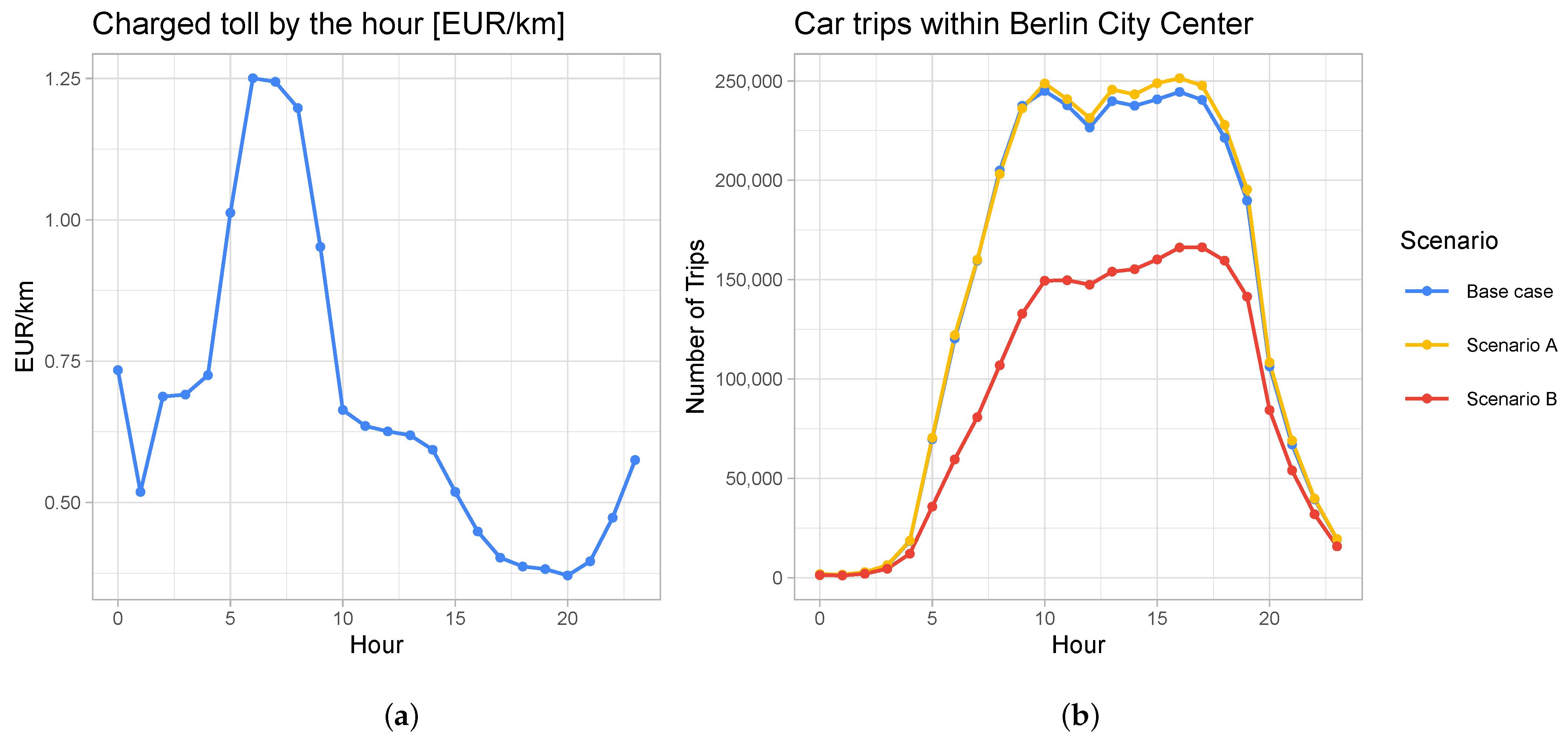
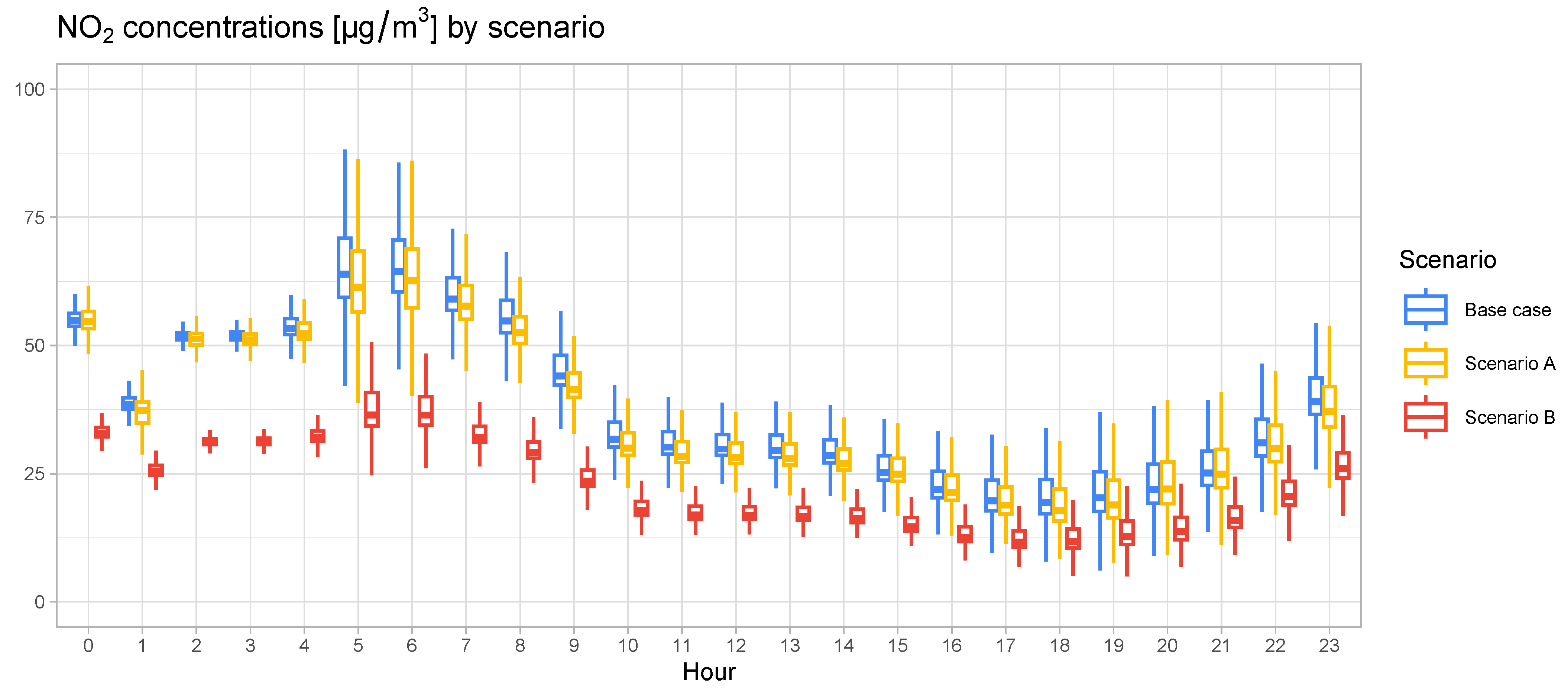
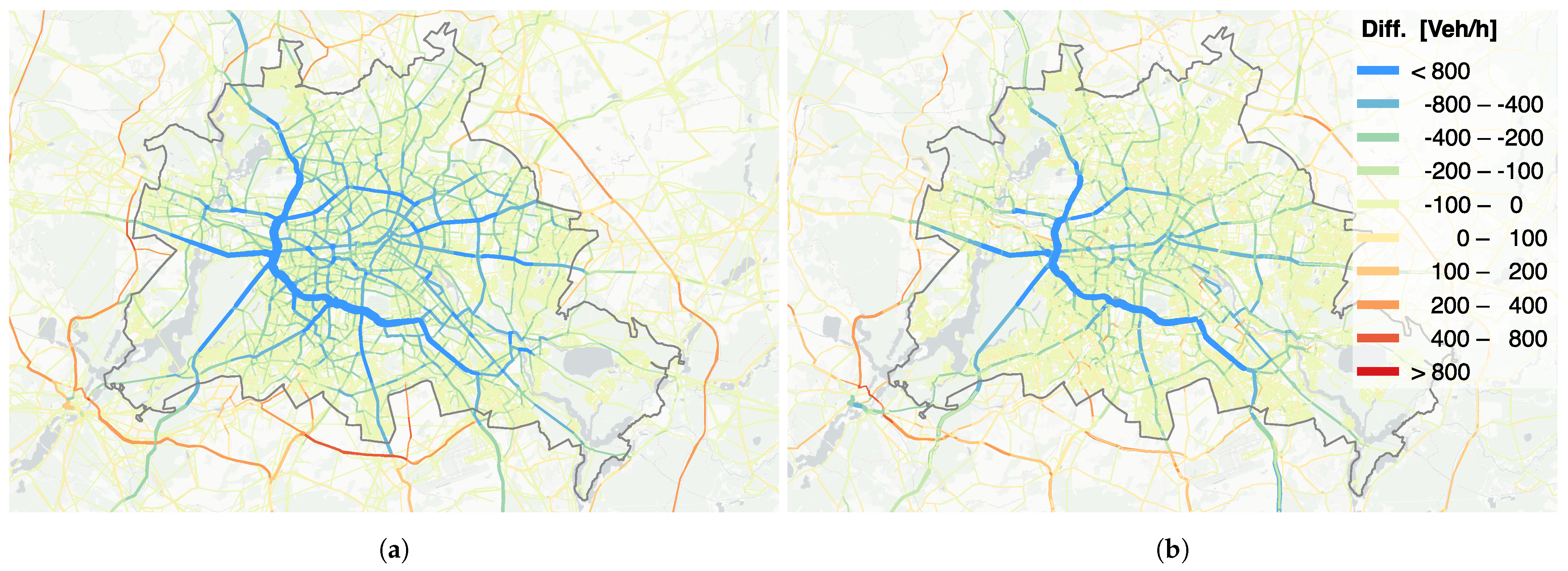
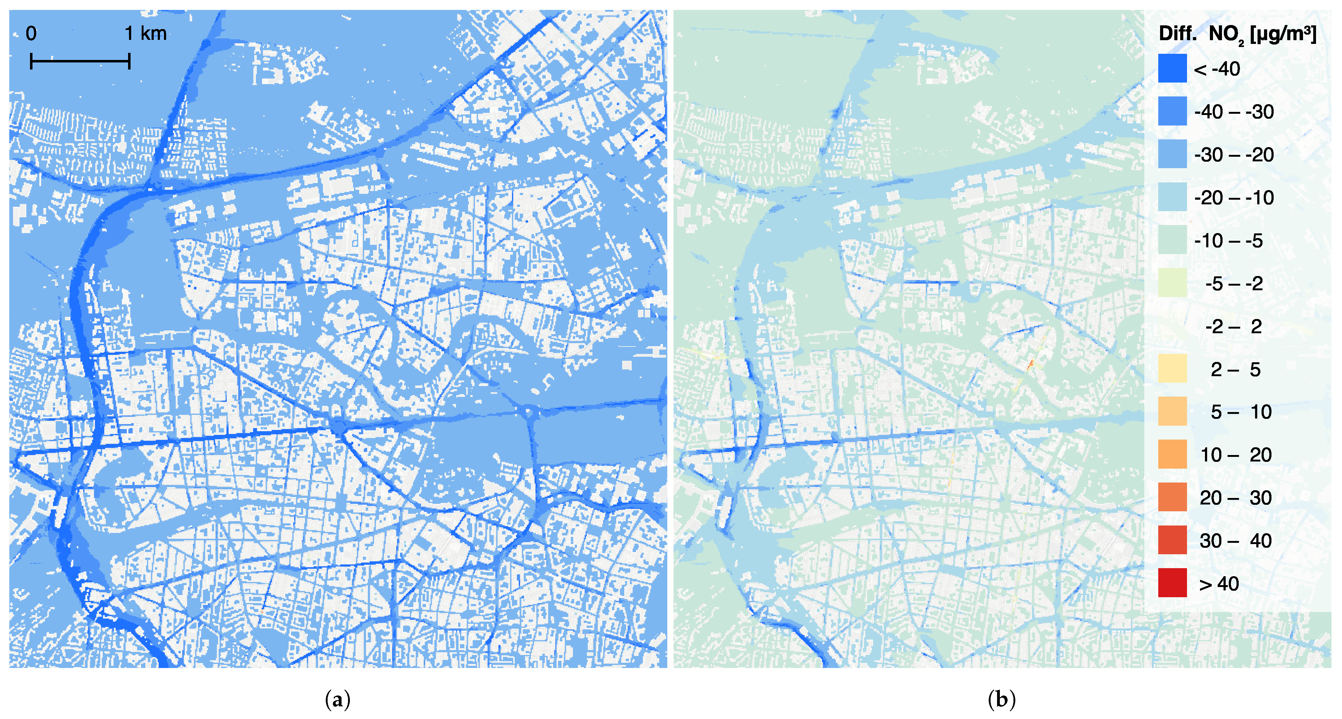
3.1. Scenario A—Toll Within the City Center

In scenario A, a toll is applied specifically to Berlin’s city center (yellow boundaries in Figure 1). Compared to the base case, the number of car trips within the Berlin area (blue boundaries in Figure 1) slightly increases, by 1%, as shown in Figure 4b. Similar to the base case, there is a morning peak between 10 am and 11 am with 248,740 trips, and an afternoon peak between 4 pm and 5 pm with 251,420 car trips. This increase in car trips may seem unexpected, but it can be explained by the smaller size of the toll area relative to the area where trips are counted.
Figure 5 shows aggregate NO2 concentration levels of the bottom layer calculated with PALM-4U for the base case, scenario A, and scenario B. Focusing on the aggregate NO2 concentrations for scenario A reveals a slight overall decrease in NO2 levels in scenario A compared to the base case. Throughout the day, NO2 concentrations in scenario A follow a pattern similar to that of the base case. A morning peak occurs between 5 am and 8 am, with median concentrations reaching up to 63 μ g/m3 between 6 am and 7 am, representing a 3% reduction compared to the base case. For the remainder of the day, median concentrations in scenario A are either similar to or up to 8% lower than those in the base case.
Despite an increase in overall car trips and only a minimal decrease in aggregate concentration levels, an inspection of spatial changes in traffic volume (Figure 6) reveals that the toll applied to the city center effectively alters traffic patterns as intended. Figure 6a illustrates traffic volume in the morning (8 am to 9 am), while Figure 6b shows traffic volume in the evening (8 pm to 9 pm).
During the morning period, with high prices, overall traffic volumes within the toll area decrease, as indicated by blue and green tones in Figure 6a. The most significant reductions occur on major roads within the city center, which originally carried high traffic volumes in the base case. The traffic volume differences shown in Figure 6 also reveal how synthetic individuals adapt to toll pricing by rerouting trips that start or end outside the toll area. To avoid the toll, they bypass the area using the inner-city highway, which experiences a substantial increase in traffic volume, with more than 800 additional vehicles per hour during the morning period.
Interestingly, certain roads located at the northern edge of the toll area show increased traffic volumes compared to the base case. Since the toll is distance-based, it may be more cost-effective for individuals to enter the toll area for trips ending near its edge. Additionally, as individuals with destinations in the center of the toll area switch to alternative modes of transportation, road capacity outside the toll area is freed up, allowing other drivers to use these roads more freely.
During the lower-priced evening period between 8 pm and 9 pm (Figure 6b), the toll’s influence on traffic patterns remains visible, but is less pronounced than during the morning. While most major roads within the toll area still see reduced traffic volumes compared to the base case, the inner-city highway continues to serve as an alternative bypass for individuals avoiding toll charges.
The changes in traffic volume are reflected in the spatial comparison of NO2 concentrations shown in Figure 7. Figure 7a presents concentration differences for the morning period (8 am to 9 am), while Figure 7b presents concentration differences for the evening period (8 pm to 9 pm).
Reflecting traffic volume changes, the morning NO2 concentrations in Figure 7a actually show increased NO2 concentrations in grid cells near the inner-city highway, particularly in the north and west of the PALM simulation domain. The highest concentration increases, between 30 μ g/m3 and 40 μ g/m3, are found in highway sections within obstructed areas, specifically in the southwest and near the center of the western boundary of the PALM simulation domain. Additionally, a section in the northeast, located within a street canyon, shows high NO2 increases, likely due to emissions carried from the highway further west.
In contrast, grid cells away from the inner-city highway show decreased morning concentrations. Major roads exhibit the largest reductions, with concentration levels decreasing by 20 to 40 μ g/m3. Particularly in the southeast of the simulation domain, some raster cells adjacent to major roads show concentration reductions of more than 40 μ g/m3, while areas farther from major roads experience smaller reductions, generally between 0 and 5 μ g/m3 compared to the base case.
The evening period (Figure 7b) presents a different pattern due to the lower toll rates, which result in less pronounced reductions in traffic volumes and thus in concentrations. Most grid cells within the toll area display minimal or modest NO2 concentration decreases, typically ranging from 0 to 20 μ g/m3 along major roads. The inner-city highway continues to experience increased traffic volumes compared to the base case, reflected in elevated NO2 concentrations, though these increases are generally smaller than in the morning, with most areas showing differences between 5 and 20 μ g/m3. However, in obstructed areas close to the inner-city highway, increases can still reach up to 40 μ g/m3, similar to the morning period. Due to the lower evening toll, some grid cells near road segments within the toll area show slight NO2 concentration increases as well, which were not present in the morning period.

3.2. Scenario B—Toll in the Berlin City Area

Imposing a time-dependent toll across the entire city of Berlin has a substantial effect on reducing car trips within Berlin’s city area (blue area in Figure 1). As shown in Figure 4b, scenario B results in a 39% decrease in trips during the morning peak compared to the base case. Specifically, between 10 am and 11 am, when the base case reaches a peak of 245,000 car trips, scenario B shows only 149,470 trips. As lower prices are charged in the afternoon hours, the peak hour shifts to the period between 5 pm and 6 pm. With 166,320 car trips compared to 240,510 trips in the base case, the number of car trips is 31% lower during the evening peak hour of scenario B. This effect can be attributed to a “lock-in” phenomenon: individuals who avoid using cars in the morning due to high toll prices are often unable to use their cars later in the day, as the vehicles are unavailable for subsequent trips. This consistent causality in the time direction is a strength of the agent-based approach [53].
The reduction in car trips within Berlin’s city area is also reflected in the aggregated pollutant concentrations from the subsequent PALM-4U simulation run, displayed in Figure 5. The introduction of a toll across the entire city area leads to a significant reduction in pollutant levels, especially in the morning. In scenario B, the largest reduction occurs between 8 am and 9 am, with median NO2 concentrations reduced by 52%, to 39.5 μ g/m3, during this period.
Figure 5 also shows that NO2 concentrations still peak in the morning between 5 am and 9 am, with median levels reaching up to 36.4 μ g/m3. Although this peak is less pronounced compared to the base case, it remains noticeable because traffic activity begins while the atmospheric boundary layer is still shallow. Aggregate NO2 concentrations for scenario B remain lower throughout the day, although the differences are less substantial after the morning peak. During midday, scenario B shows reductions of 41% to 44%, with median concentrations between 12.6 μ g/m3 and 17.8 μ g/m3. In the evening and night hours, the difference between scenario B and the base case decreases to 34%, with median NO2 concentrations in scenario B ranging between 11.7 μ g/m3 and 26 μ g/m3, showing only a slight decrease from the afternoon, before concentration levels increase at night hours.
Inspecting the aggregate concentration levels for scenario B and the base case in Figure 5 confirms that the introduced toll is effective in reducing concentration peaks during morning hours. Additionally, air pollution concentrations are lowered throughout the remaining hours of the day.
The differentiation in toll prices is also evident when examining changes in traffic volumes for the morning period (8–9 am) in Figure 8a, and the evening period (8–9 pm) in Figure 8b. The figures reveal that the synthetic population adjusts its behavior in response to the toll. Car trips with a start and/or destination within the toll area are replaced by alternative modes of transportation, primarily public transit and bicycles. For trips passing through the toll area, affected individuals often select alternative routes to avoid the toll, resulting in increased traffic on highways surrounding Berlin. A comparison of Figure 8a,b also shows that reductions in traffic volumes within the toll area are more pronounced in the morning than in the evening, a pattern similarly observed in the increased traffic volumes on highways outside Berlin.
This effect is further reflected in the changes in pollutant concentration values simulated with the PALM-4U model. Figure 9 depicts average NO2 concentration values for the same periods as Figure 8, with concentrations between 8 am and 9 am in Figure 9a and between 8 pm and 9 pm in Figure 9b. Simulated morning concentrations are significantly lower across the entire PALM-4U model domain compared to the base case. The greatest reductions can be observed on the inner-city highway in the western part of the domain, where NO2 levels are reduced by over 40 μ g/m3 on most sections of the highway. Simulated morning concentrations (Figure 9a) on arterial roads show reductions of comparable magnitude. In contrast, areas not adjacent to major roads show reductions in NO2 concentrations between 20 μ g/m3 and 30 μ g/m3.
In the evening period, shown in Figure 9b, the picture is less uniform. The most significant reductions in NO2 concentrations still occur along the inner-city highway in the western domain, though reductions are smaller than those in the morning, generally ranging between 10 μ g/m3 and 40 μ g/m3. A few places along the highway also show decreases in concentration levels greater than 40 μ g/m3. These are generally located in obstructed areas, where air pollution is trapped in turbulence forming in street canyons. Reductions in air pollution levels are also observed for raster cells close to major roads, where NO2 concentrations decrease by 10 μ g/m3 to 40 μ g/m3. Further away from major roads, reductions in NO2 concentrations remain visible, but are less pronounced compared to the base case. The overall spatial pattern aligns with the aggregate concentration values shown in Figure 5, where median concentration differences are most notable during the morning hours.
Interestingly, Figure 9b reveals a few raster cells with higher NO2 concentrations than the base case. These cells are located close to road segments with increased traffic volumes during the evening hours, as can be seen in Figure 8b. Additionally, the cells with increased NO2 concentrations are located in street canyons that are perpendicular to the prevailing wind direction. In such street canyons, eddies form, trapping pollution within the canyon and leading to locally higher concentrations.

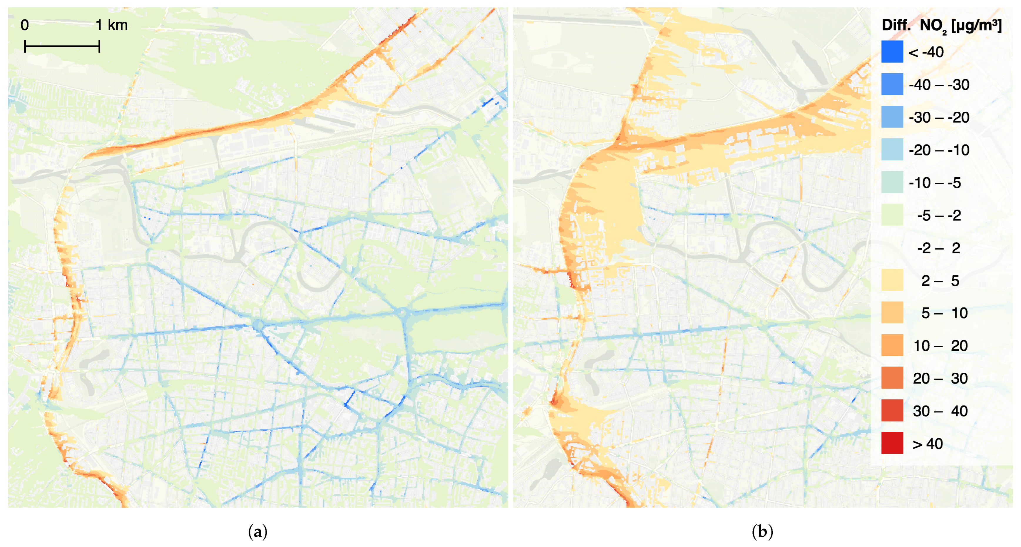
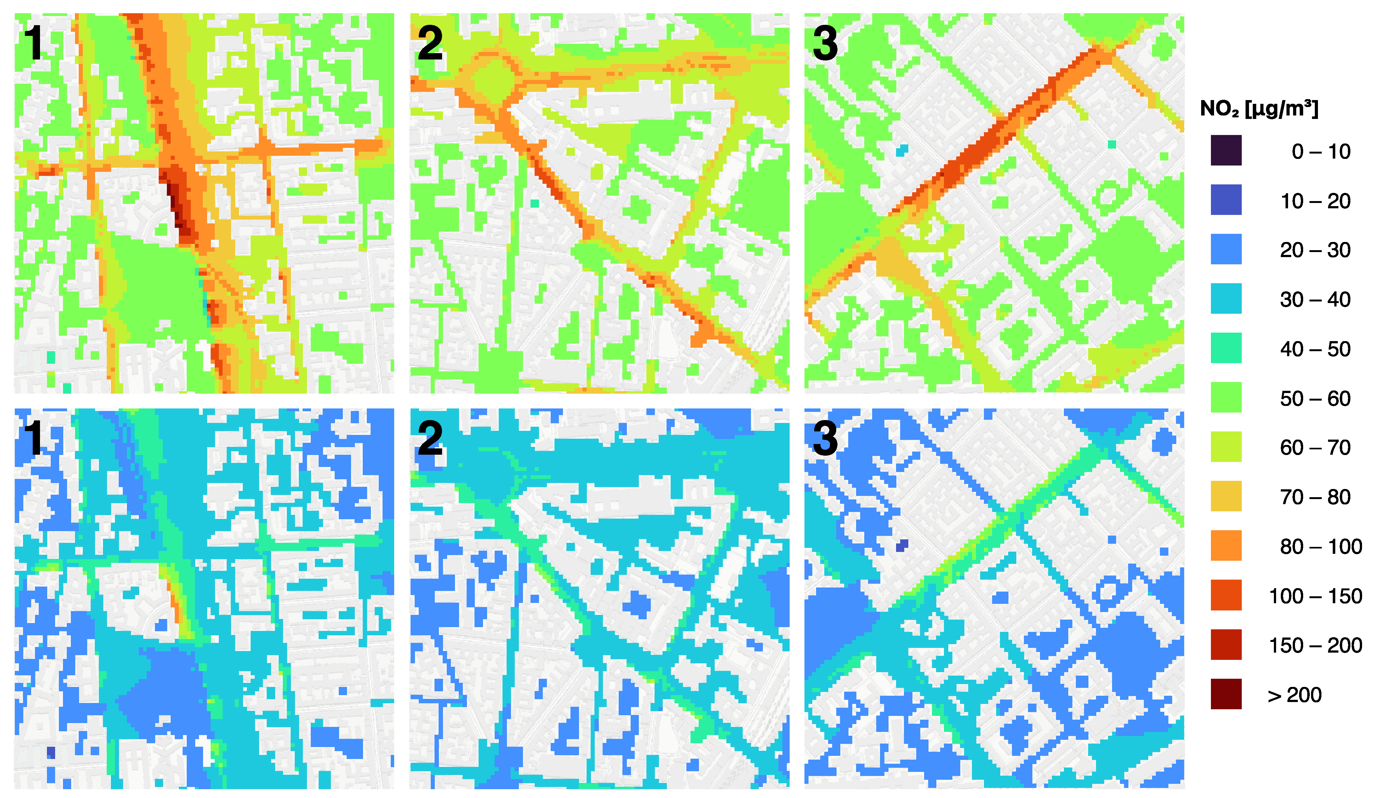
3.3. Scenario B—Spatial Hotspot Mitigation

Scenario B shows reduced NO2 concentrations across the entire PALM-4U simulation domain in response to the citywide toll scheme. To show the advantages of using a high-resolution LES CFD model, we analyze three locations with high NO2 concentrations between 7 am and 8 am. These areas, marked as 1, 2, and 3 in Figure 2a, represent air pollution hotspots in different urban locations, with particularly high concentration levels. Figure 10 compares NO2 concentrations for the base case (top) and scenario B (bottom) in these sections.
Section 1 is located along the inner-city highway on the western side of the PALM-4U simulation domain. In the base case, NO2 concentrations exceed 200 μ g/m3 within a restricted area of the section, reflecting high traffic volumes and emissions. The observed concentrations are also a result of the stationary setup used in the artificial case study. Under realistic meteorological conditions, lower concentration levels can be expected. The highway is situated within a street canyon obstructed by buildings, which is aligned perpendicular to the wind direction. Turbulence within the canyon generates eddies that trap emissions and transport them toward the windward side of the street canyon, resulting in high pollution concentrations. Under scenario B, NO2 concentrations in Section 1 are significantly reduced. Peak values decrease by approximately 50%, ranging between 81 μ g/m3 and 94 μ g/m3. Notably, sections of the highway outside the canyon show concentrations similar to surrounding areas, ranging between 35 μ g/m3 and 45 μ g/m3.
Section 2 covers a major arterial road in Berlin’s city center, situated diagonally to the prevailing wind and enclosed by buildings on both sides. In the base case, concentrations inside the street canyon range from 76 μ g/m3 to 124 μ g/m3. The high-resolution LES CFD simulation captures turbulence within the canyon, transporting emissions toward the windward side of the street. In scenario B, concentrations are reduced by approximately 50%, with peak values of 56 μ g/m3. Despite the reductions, the spatial distribution of NO2 remains similar, as turbulence continues to concentrate pollutants on the windward side of the canyon.
Section 3 focuses on a major street in the northeast of the simulation domain, also located in a street canyon. Unlike sections 1 and 2, NO2 concentrations in Section 3 are distributed more evenly, suggesting that the pollutants are transported along the canyon’s length rather than being trapped by eddies. In the base case, concentrations range from 89 μ g/m3 to 134 μ g/m3. Under scenario B, concentrations decrease by approximately 50%, falling within a range of 41 μ g/m3 to 68 μ g/m3. The overall distribution of air pollution concentrations, is similar to the base case, with pollutants being transported along the street canyon. In areas with lower overall concentrations, concentration maxima can be observed on the windward side of the street canyon; these are less pronounced compared to Section 1 and Section 2.
This analysis of spatial hotspots demonstrates that the LES CFD simulation effectively captures concentration dynamics at high resolution, incorporating wind-induced turbulence and urban canopy effects. Importantly, the 50% reduction observed in the aggregate analysis for scenario B (Figure 5) is also evident on a micro level. These findings highlight the effectiveness of coupling a traffic model with a high-resolution CFD emission model, enabling a detailed assessment of how macro-level policy measures translate into localized environmental impacts.

4. Discussion

The presented case study implements a feedback-driven traffic management policy, based on air pollution data simulated with PALM-4U. The initial pollution data are obtained by using traffic emissions generated with MATSim as input for the PALM-4U simulation setup. By integrating air pollution concentration data directly into the policy design, we create a system where traffic management policies can respond to environmental conditions.

4.1. Limitations

The simulations in this study assume constant meteorological conditions, such as steady wind speeds and directions. This assumption is made to emphasize the impact of traffic emissions, isolating them as the primary variable under study. However, it does not capture the variability in real-world weather patterns, which can significantly influence pollutant dispersion.
The toll rates applied in this study are artificially scaled to amplify behavioral responses in the simulation. While this scaling effectively demonstrates the coupling mechanism’s capabilities, it may not reflect realistic economic or policy scenarios. A pricing which is more oriented towards actual damage costs caused by road traffic would be more realistic.
This study primarily focuses on NO2 concentrations, with limited consideration of other pollutants such as ultra-fine particulate matter (PM2.5) or ozone. A more comprehensive understanding of the relation between road traffic and its influence on urban air quality requires the assessment of these species as well.
Additionally, due to its high computational costs, the model domain covered by the PALM-4U setup remains limited. While MATSim allows for the simulation of traffic patterns for the entire city of Berlin, its influence on the urban climate can only be predicted for a part of the city. This limitation might be overcome with advancements in computational capabilities in the future. However, operating a model at an even larger scale requires personnel with significant high-performance computing expertise.

4.2. Advantages

The presented methodology uniquely combines MATSim’s traffic simulation capabilities with the PALM-4U urban climate model’s high-resolution pollutant dispersion simulations. This dual-model approach enables precise assessments of how traffic management policies influence air quality, capturing both temporal and spatial variations in pollutant concentrations. The use of a turbulence-resolving LES model in PALM-4U provides a granular understanding of pollutant dynamics within urban environments. This high resolution enables the accurate identification of pollution hotspots and their underlying causes, such as wind-induced turbulence in street canyons.
The inclusion of a feedback mechanism enables the design of traffic management policies that directly address air pollution levels simulated with PALM-4U. This enables the evaluation of such policies’ effectiveness on air pollution concentrations. The presented methodology extends beyond the specific policy demonstrated in our case study, which focuses on the mitigation of temporal concentration peaks. The introduced feedback loop between both models allows for testing of the impact of different strategies on air quality to improve the situation for urban residents.
The combined approach enables a quantitative discussion of the objectives behind air quality improvement measures. For instance, it allows for a discussion of critical questions, such as whether measurement stations should be placed at locations with the highest concentrations or at more representative typical urban locations. Additionally, it prompts a broader evaluation of whether efforts should aim to ensure all locations remain below certain legal thresholds or to minimize overall population exposure and associated health impacts. Addressing these questions would clarify objectives and provide insights into the differences in population health outcomes between these strategies.
Finally, the methodology’s reliance on open-source software and data enhances its adaptability. MATSim, PALM-4U-4U, and supplementary tools, as well as the use of OSM for input data, ensure that the framework can be applied to other urban regions. This flexibility makes the approach particularly suitable for replication in cities worldwide, facilitating widespread adoption of evidence-based traffic management strategies.

4.3. Comparison and Advancements over Existing Work

To contextualize our approach, we compare it to relevant studies that integrate traffic emissions with air quality modeling or implement emissions-based traffic management strategies.
San José et al. [36] couple the microscopic traffic model SUMO with the high-resolution CFD model MICROSYS-CFD to simulate traffic-induced air pollution in urban environments. While their work successfully models air pollution from traffic emissions, it does not include a feedback mechanism to integrate traffic management policies, limiting its adaptability for designing responsive interventions. In contrast, our approach extends this capability by introducing a feedback loop that evaluates and adjusts traffic management strategies based on modeled pollution levels. Furthermore, their use of a RANS CFD model identifies pollution maxima on the downwind side of street canyons but lacks the turbulence-resolving accuracy of our LES-based modeling. By resolving turbulence explicitly, our approach improves the precision of predicting high-concentration hotspots, as illustrated in Section 3.3.
The study by Agarwal and Kickhöfer [54] implements a comprehensive traffic management strategy that internalizes the external costs of traffic emissions and congestion. Their approach calculates external costs for each vehicle on each street segment and charges drivers accordingly, encouraging route or mode changes. This methodology is similar to our initial approach, which also attributes costs at the street-segment level to influence individual travel behavior. However, their results show consistently high pollution concentrations near busy road segments, regardless of the time of day. This is due to their use of a simplified dispersion model, which does not account for temporal variations in pollutant dispersion or the influence of urban canopy geometry. In contrast, our approach, which incorporates a turbulence-resolving LES model, provides more nuanced results. While we also observe high concentrations near busy roads, our findings reveal significant temporal variations throughout the day and spatial differences influenced by the urban canopy layout. These differences highlight the importance of high-resolution dispersion modeling for accurately assessing air quality and exposure levels.
Finally, Samad et al. [38] conduct a sophisticated PALM simulation with multi-level nesting of model domains in a case study for Stuttgart, implementing a policy where older diesel vehicles are replaced with cleaner ones. Their work demonstrates excellence in CFD modeling and highlights the sensitivity of PALM to emission changes. However, their approach assumes a uniform reduction in emissions across all streets, as it does not account for traffic pattern shifts or route-based restrictions typical of real-world scenarios. In contrast, our methodology integrates a behavior-based traffic model, enabling the simulation of dynamic traffic shifts in response to policies such as cordon-based tolls. This allows us to more accurately capture the interplay between emissions regulations and real-world traffic behavior, as demonstrated in Section 3.1. By modeling these interactions, our approach provides more realistic insights into the potential outcomes of traffic management policies.
In summary, our approach extends the referenced work by integrating a responsive feedback loop, accounting for temporal variations in pollution concentrations, and capturing realistic shifts in traffic behavior. This combination allows for more effective, nuanced, and practical traffic management policy evaluations in urban environments.

5. Conclusions and Outlook

This paper investigates how high-resolution urban climate modeling can be used to address air pollution hotspots in urban areas. By coupling the CFD-LES model PALM-4U and the traffic simulation MATSim we showcase an integrated approach for designing and evaluating traffic management policies. Our initial idea to trace areas with high concentrations back to nearby links with high emissions had to be rejected due to the complexity of turbulent airflow dynamics revealed by the high-resolution LES-CFD model. Instead, the height of the atmospheric boundary layer has a dominating effect: during the morning hours, the boundary layer is shallow, causing pollutants to concentrate in a smaller air volume and resulting in high concentrations. Conversely, during midday, the boundary layer expands, and traffic emissions are dispersed into a larger air volume, leading to lower concentrations. Consequently, if the goal is to reduce short-term concentration hotspots, mitigation efforts should prioritize the morning period.
To illustrate these findings with a practical traffic management measure, we apply a toll that is spatially uniform but temporally proportional to pollutant concentrations. The traffic model is re-run with this tolling scheme, followed by a re-run of the high-resolution urban climate model. This analysis reveals the importance of setting the tolled area large enough to avoid even higher air pollution concentrations in hotspots near the boundaries of the tolled zone.
Future work should investigate real-world applications of this framework, featuring realistic meteorological conditions. This includes the design of traffic management policies tailored to various weather scenarios, such as different wind directions and temperature variations.
Given that the ultimate aim of air pollution mitigation is to reduce adverse health effects, the proposed coupling mechanism should be expanded to assess exposure to air pollution. Since activity locations and trajectories of synthetic individuals are available in MATSim, it should be feasible to design traffic management policies that minimize the population’s exposure to air pollution, based on existing research on individual air pollution exposure [5,55,56]. Additionally, the generated air pollution concentration data could be used as input to estimate the health impact on the population level [57,58].
The possibilities arising from the coupling of MATSim and PALM-4U have not yet been fully exploited, especially regarding the level of detail used. Instead of temporally aggregated traffic emissions, it is possible to determine vehicle positions and their emissions in MATSim with second-by-second precision and use these as input data for pollutant dispersion calculations in PALM-4U. This approach is currently under development.

Author Contributions

Conceptualization, J.L., S.B. and K.N.; data curation, J.L., S.B. and B.K.; formal analysis, J.L., S.B. and K.N.; funding acquisition, K.N.; investigation, J.L. and S.B.; methodology, J.L., S.B. and K.N.; project administration, K.N.; resources, K.N.; software, J.L. and B.K.; supervision, K.N.; validation, J.L., S.B. and K.N.; visualization, J.L.; writing—original draft, J.L.; writing—review and editing, S.B. and K.N. All authors have read and agreed to the published version of the manuscript.

Funding

This work was partially funded by the BMBF—Bundesministerium für Bildung und Forschung grant number 01LP1911C.

Institutional Review Board Statement

Not applicable.

Informed Consent Statement

Not applicable.

Data Availability Statement

The conversion tool used in this article can be found at https://gitlab.palm-model.org/matsim/matsim_traffic_emmisions/-/tree/mosaik-2-01 (17 December 2024), an open-source git repository hosted as part of the PALM model system and was run with the version captured in [47]. The MATSim setup can be found at https://github.com/matsim-scenarios/matsim-berlin/releases/tag/mosaik-2-01 (17 December 2024) and was run with the MosaikRunner.java class [48]. The original PALM-4U setup can be found at https://doi.org/10.5281/zenodo.4020560 (24 January 2025), a data repository stored at the Zenodo project [59]. All input and output data related to this article can be found at https://doi.org/10.14279/depositonce-18737 (17 December 2024), a data repository hosted at Technische Universität Berlin [60].

Acknowledgments

The authors gratefully acknowledge the computing time made available to execute the PALM-4U setup on the high-performance computer “Lise” at the NHR Center NHR@ZIB. This center is jointly supported by the Federal Ministry of Education and Research and the state governments participating in the NHR (www.nhr-verein.de/unsere-partner (17 December 2024)). Map data of background maps are copyrighted by OpenStreetMap contributors and available from https://www.openstreetmap.org (19 January 2025).

Conflicts of Interest

The authors declare no conflicts of interest.

Abbreviations

ADMSAtmospheric Dispersion Modelling System
BEVBattery electric vehicle
CALINEA line source air quality dispersion model
CFDComputational fluid dynamics
CMEMComprehensive Modal Emission Model
COPERTComputer Programme to Calculate Emissions from Road Transport
EMITEnvironmental Model of Individual Traffic
EUEuropean Union
GTFSGeneral Transit Feed Specification
HBEFAHandbook Emission Factors for Road Transport
HECTHandbook on the External Costs of Transport
HPCHigh-performance computing
IMMISIntegrated Model for the Management of Traffic-related Emissions
LESLarge-eddy simulation
LODLevel of detail
MATSimMulti-Agent Transport Simulation
MOVESMotor Vehicle Emission Simulator
NONitrogen monoxide
NO2Nitrogen dioxide
NOxNitrogen oxides
O3Ozone
OSMOpenStreetMap
OSPMOperational Street Pollution Model
PTPublic transit
RANSReynolds-averaged Navier–Stokes
RLINEA dispersion model for near-road applications

Appendix A

As detailed in Section 2.6, grid cells close to roads with high traffic volumes generally show higher pollutant concentrations than those further away from streets. The initial approach for traffic management is to identify street segments that lead to particularly high pollutant concentrations in the urban climate model. Then, the intention is to impose a time and distance-based toll on these links to decrease traffic volume and thus pollutant emissions. For this approach, we assume that links with high traffic volume and close proximity to a grid cell have a greater impact on pollutant concentration within the grid cell than more distant links with lower traffic volume. Using the simplified dispersion model mentioned in Section 2.2 in reverse, observed concentrations in a grid cell can be attributed to surrounding links, depending on their distance to that grid cell.
As a first test for this approach, a correlation between the simplified Gaussian dispersion model and the concentrations generated with PALM-4U is investigated. Since pollutant concentrations calculated with the simplified dispersion model directly depend on the traffic volumes of the surrounding links, this would also establish a relationship between pollutant concentrations calculated by PALM-4U and traffic volumes simulated with MATSim. However, the results show only a weak correlation between pollutant concentrations from PALM-4U and those generated using the simplified Gaussian model.
Figure A1 shows the correlation between NOx concentrations from the MATSim baseline scenario and the corresponding PALM-4U run for different hours of the day. Each data point represents a raster cell in the PALM-4U domain. The x-axis displays NOx values from the simplified Gaussian model, while the y-axis shows NOx concentrations from PALM-4U. The y-axis is limited to 500 μ g/m3, and values above this limit (0.3% of the data) are excluded as outliers. Linear fits, based on a standard linear model, are applied for each hour and shown as blue lines in Figure A1.
The scatter plots reveal certain patterns for different hours of the day. Most points cluster densely at lower values in both models, with the PALM-4U simulation showing a slight upward trend for higher concentrations predicted by the simplified Gaussian model. However, beyond these dense clusters, the data points are widely scattered, showing no clear correlation between the two models.
While some structure is visible—such as the dense point cloud at lower values and a line formed by the PALM-4U simulation for higher concentrations—the blue trend lines fail to capture these patterns. The linear fits generally have steeper slopes than the main clusters and do not represent the scattered distribution of values. This highlights that the expected linear correlation between the two models cannot be assumed.
Figure A1. Hourly concentrations from the MATSim baseline scenario distributed across the grid of the PALM-4U simulation domain (x-axis). A Gaussian blur was applied to distribute the emissions. In comparison, hourly concentrations from the corresponding PALM-4U run (y-axis). A linear regression for each hour is shown in blue.
Atmosphere 16 00128 g0a1
Despite the missing correlation, two key observations can be made from Figure A1:
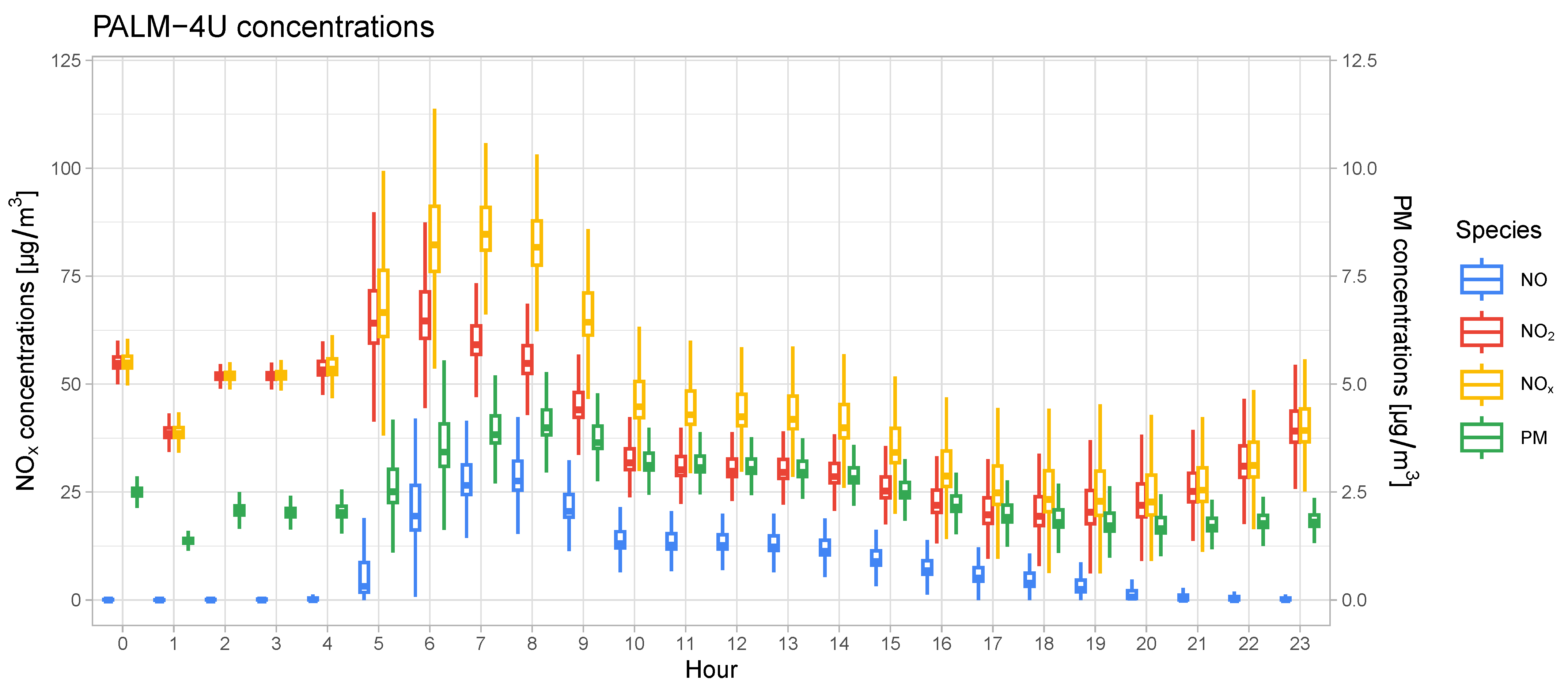
  • A minimum threshold for NOx concentrations from the PALM-4U simulation is visible. This threshold changes throughout the day, being higher in the morning and lower in the afternoon.
  • The upper boundary of the point cloud for NOx values from PALM-4U also changes over time. In the morning, NOx values are more spread out and reach higher levels. In the afternoon, the spread is smaller, and the upper boundary is lower.
These findings align with our previous work, where we identify additional factors as stronger determinants of pollutant concentrations than proximity to high-traffic street segments Laudan et al. [13]. The four key factors influencing pollutant concentrations, are summarized here:
  • Street layout and dispersion—Street alignment relative to the wind direction strongly influences pollutant dispersion. On streets parallel to wind flow, pollutants tend to disperse in the downwind direction, resulting in lower concentrations. In contrast, perpendicular streets within densely developed areas show elevated concentrations on the upwind side. On streets surrounded by minimal development, pollution is dispersed in the downwind direction, leading to lower concentrations as well.
  • Boundary layer—The boundary layer expands after sunrise and shrinks again after sunset. This means that pollutants are diluted in a much smaller air volume at the beginning and end of the day compared to midday, leading to much higher concentrations for the same traffic volume at the start of the day.
  • Air chemistry—Chemical transformations, such as the photolysis of NO2 under sunlight, impact pollutant concentration levels. These reactions are sensitive to sunlight, which varies throughout the day.
  • Geometric artifacts—Converting street canyons to a grid-based format introduces stepped surfaces that do not accurately reflect smooth canyon walls, causing fluctuations in canyon width. This artifact results in small-scale concentration anomalies within the grid cells, leading to outliers in pollutant concentrations.
Based on the results of the investigation, the traffic management policy is shifted from a traffic volume-based approach to the time-based strategy outlined in Section 2.6.

References

  1. Ciarelli, G.; Colette, A.; Schucht, S.; Beekmann, M.; Andersson, C.; Manders-Groot, A.; Mircea, M.; Tsyro, S.; Fagerli, H.; Ortiz, A.G.; et al. Long-term health impact assessment of total PM2.5 in Europe during the 1990–2015 period. Atmos. Environ. X 2019, 3, 100032. [Google Scholar] [CrossRef]
  2. European Environment Agency. Air Quality in Europe: 2020 Report; Publications Office of the European Union: Luxembourg, 2020. [Google Scholar]
  3. Schulz, H.; Karrasch, S.; Bölke, G.; Cyrys, J.; Hornberg, C.; Pickford, R.; Schneider, A.; Witt, C.; Hoffmann, B. Atmen. DGfPuB eV Deutsche Gesellschaft für Pneumologie und Beatmungsmedizine. V., Berlin. 2018. Available online: https://www.pneumologeninsachsen.de/fileadmin/template/downloads/Oeffentlicher_Bereich/Pressemitteilungen/DGP_Luftschadstoffe_Positionspapier_20190129.pdf (accessed on 24 January 2024).
  4. Desa, U.N. World Urbanization Prospects 2018: Highlights; Technical report; United Nations: New York, NY, USA, 2018. [Google Scholar]
  5. Dons, E.; Int Panis, L.; Van Poppel, M.; Theunis, J.; Willems, H.; Torfs, R.; Wets, G. Impact of time–activity patterns on personal exposure to black carbon. Atmos. Environ. 2011, 45, 3594–3602. [Google Scholar] [CrossRef]
  6. Ma, X.; Zou, B.; Deng, J.; Gao, J.; Longley, I.; Xiao, S.; Guo, B.; Wu, Y.; Xu, T.; Xu, X.; et al. A comprehensive review of the development of land use regression approaches for modeling spatiotemporal variations of ambient air pollution: A perspective from 2011 to 2023. Environ. Int. 2024, 183, 108430. [Google Scholar] [CrossRef] [PubMed]
  7. McConnell, R.; Islam, T.; Shankardass, K.; Jerrett, M.; Lurmann, F.; Gilliland, F.; Gauderman, J.; Avol, E.; Künzli, N.; Yao, L.; et al. Childhood incident asthma and traffic-related air pollution at home and school. Environ. Health Perspect. 2010, 118, 1021–1026. [Google Scholar] [CrossRef] [PubMed]
  8. Hoek, G.; Beelen, R.; de Hoogh, K.; Vienneau, D.; Gulliver, J.; Fischer, P.; Briggs, D. A review of land-use regression models to assess spatial variation of outdoor air pollution. Atmos. Environ. (1994) 2008, 42, 7561–7578. [Google Scholar] [CrossRef]
  9. Gürbüz, H.; Şöhret, Y.; Ekici, S. Evaluating effects of the COVID-19 pandemic period on energy consumption and enviro-economic indicators of Turkish road transportation. Energy Sources Part Recover. Util. Environ. Eff. 2021, 1–13. [Google Scholar] [CrossRef]
  10. von Schneidemesser, E.; Sibiya, B.; Caseiro, A.; Butler, T.; Lawrence, M.G.; Leitao, J.; Lupascu, A.; Salvador, P. Learning from the COVID-19 lockdown in berlin: Observations and modelling to support understanding policies to reduce NO2. Atmos. Environ. X 2021, 12, 100122. [Google Scholar] [CrossRef] [PubMed]
  11. Horni, A.; Nagel, K.; Axhausen, K.W. The Multi-Agent Transport Simulation Matsim; Ubiquity Press: London, UK, 2016. [Google Scholar] [CrossRef]
  12. Maronga, B.; Banzhaf, S.; Burmeister, C.; Esch, T.; Forkel, R.; Fröhlich, D.; Fuka, V.; Gehrke, K.F.; Geletič, J.; Giersch, S.; et al. Overview of the PALM model system 6.0. Geosci. Model Dev. 2020, 13, 1335–1372. [Google Scholar] [CrossRef]
  13. Laudan, J.; Banzhaf, S.; Khan, B.; Nagel, K. Coupling MATSim and the PALM model system—Large scale traffic and emission modeling with high-resolution computational fluid dynamics dispersion modeling. Atmosphere 2024, 15, 1183. [Google Scholar] [CrossRef]
  14. Mądziel, M. Vehicle Emission Models and Traffic Simulators: A Review. Energies 2023, 16, 3941. [Google Scholar] [CrossRef]
  15. Forehead, H.; Huynh, N. Review of modelling air pollution from traffic at street-level—The state of the science. Environ. Pollut. 2018, 241, 775–786. [Google Scholar] [CrossRef] [PubMed]
  16. Ma, X.; Lei, W.; Andréasson, I.; Chen, H. An Evaluation of Microscopic Emission Models for Traffic Pollution Simulation Using On-board Measurement. Environ. Model. Assess. 2012, 17, 375–387. [Google Scholar] [CrossRef]
  17. Ntziachristos, L. COPERT III Computer Programme to Calculate Emissions from Road Transport: Methodology and Emission Factors (Version 2.1); European Environment Agency: Copenhagen, Denmark, 2000. [Google Scholar]
  18. Epa, U.S. Overview of EPA’s MOtor Vehicle Emission Simulator (MOVES3); U.S. Environmental Protection Agency: Washington, DC, USA, 2021.
  19. Scora, G.; Barth, M. Comprehensive modal emissions model (cmem), version 3.01. In User Guide; Centre for Environmental Research and Technology, University of California: Riverside, CA, USA, 2006; Volume 1070, p. 1580. [Google Scholar]
  20. Cappiello, A.; Chabini, I.; Nam, E.K.; Lue, A.; Abou Zeid, M. A statistical model of vehicle emissions and fuel consumption. In Proceedings of the IEEE 5th International Conference on Intelligent Transportation Systems, Singapore, 6 September 2002; pp. 801–809. [Google Scholar] [CrossRef]
  21. Johnson, J.B. An Introduction to Atmospheric Pollutant Dispersion Modelling. Environ. Sci. Proc. 2022, 19, 18. [Google Scholar] [CrossRef]
  22. Liang, M.; Chao, Y.; Tu, Y.; Xu, T. Vehicle Pollutant Dispersion in the Urban Atmospheric Environment: A Review of Mechanism, Modeling, and Application. Atmosphere 2023, 14, 279. [Google Scholar] [CrossRef]
  23. Vardoulakis, S.; Fisher, B.E.A.; Pericleous, K.; Gonzalez-Flesca, N. Modelling air quality in street canyons: A review. Atmos. Environ. 2003, 37, 155–182. [Google Scholar] [CrossRef]
  24. Benson, P.E. A review of the development and application of the CALINE3 and 4 models. Atmos. Environ. Part Urban Atmos. 1992, 26, 379–390. [Google Scholar] [CrossRef]
  25. Snyder, M.G.; Venkatram, A.; Heist, D.K.; Perry, S.G.; Petersen, W.B.; Isakov, V. RLINE: A line source dispersion model for near-surface releases. Atmos. Environ. 2013, 77, 748–756. [Google Scholar] [CrossRef]
  26. Berkowicz, R.; Hertel, O.; Larsen, S.E.; Soerensen, N.N.; Nielsen, M. Modelling Traffic Pollution in Streets; Technical Report; National Environmental Research Institute: Copenhagen, Denmark, 1997.
  27. Carruthers, D.J.; Holroyd, R.J.; Hunt, J.C.R.; Weng, W.S.; Robins, A.G.; Apsley, D.D.; Thompson, D.J.; Smith, F.B. UK-ADMS: A new approach to modelling dispersion in the earth’s atmospheric boundary layer. J. Wind Eng. Ind. Aerodyn. 1994, 52, 139–153. [Google Scholar] [CrossRef]
  28. Diegmann, V. Handbuch_Immisluft_5_2.pdf; IVU Umwelt GmbH: Breisgau, Germany, 2011. [Google Scholar]
  29. Wendt, J. Computational Fluid Dynamics: An Introduction; Springer Science & Business Media: Berlin/Heidelberg, Germany, 2008. [Google Scholar]
  30. Tominaga, Y.; Stathopoulos, T. Ten questions concerning modeling of near-field pollutant dispersion in the built environment. Build. Environ. 2016, 105, 390–402. [Google Scholar] [CrossRef]
  31. Khan, B.; Banzhaf, S.; Chan, E.C.; Forkel, R.; Kanani-Sühring, F.; Ketelsen, K.; Kurppa, M.; Maronga, B.; Mauder, M.; Raasch, S.; et al. Development of an atmospheric chemistry model coupled to the PALM model system 6.0: Implementation and first applications. Geosci. Model Dev. 2021, 14, 1171–1193. [Google Scholar] [CrossRef]
  32. Ioannidis, G.; Li, C.; Tremper, P.; Riedel, T.; Ntziachristos, L. Application of CFD Modelling for Pollutant Dispersion at an Urban Traffic Hotspot. Atmosphere 2024, 15, 113. [Google Scholar] [CrossRef]
  33. Zhang, Y.; Ye, X.; Wang, S.; He, X.; Dong, L.; Zhang, N.; Wang, H.; Wang, Z.; Ma, Y.; Wang, L.; et al. Large-eddy simulation of traffic-related air pollution at a very high resolution in a mega-city: Evaluation against mobile sensors and insights for influencing factors. Atmos. Chem. Phys. 2021, 21, 2917–2929. [Google Scholar] [CrossRef]
  34. Zheng, X.; Yang, J. Impact of moving traffic on pollutant transport in street canyons under perpendicular winds: A CFD analysis using large-eddy simulations. Sustain. Cities Soc. 2022, 82, 103911. [Google Scholar] [CrossRef]
  35. Woodward, H.; Stettler, M.; Pavlidis, D.; Aristodemou, E.; ApSimon, H.; Pain, C. A large eddy simulation of the dispersion of traffic emissions by moving vehicles at an intersection. Atmos. Environ. 2019, 215, 116891. [Google Scholar] [CrossRef]
  36. San José, R.; Pérez, J.L.; Gonzalez-Barras, R.M. Assessment of mesoscale and microscale simulations of a NO2 episode supported by traffic modelling at microscopic level. Sci. Total Environ. 2021, 752, 141992. [Google Scholar] [CrossRef] [PubMed]
  37. Sanchez, B.; Santiago, J.L.; Martilli, A.; Martin, F.; Borge, R.; Quaassdorff, C.; de la Paz, D. Modelling NOX concentrations through CFD-RANS in an urban hot-spot using high resolution traffic emissions and meteorology from a mesoscale model. Atmos. Environ. 2017, 163, 155–165. [Google Scholar] [CrossRef]
  38. Samad, A.; Caballero Arciénega, N.A.; Alabdallah, T.; Vogt, U. Application of the Urban Climate Model PALM-4U to Investigate the Effects of the Diesel Traffic Ban on Air Quality in Stuttgart. Atmosphere 2024, 15, 111. [Google Scholar] [CrossRef]
  39. Kaddoura, I. Simulated Dynamic Pricing for Transport System Optimization. Ph.D. Thesis, Technische Universitaet Berlin, Berlin, Germany, 2019. [Google Scholar] [CrossRef]
  40. Xiong, C.; Zhu, Z.; He, X.; Chen, X.; Zhu, S.; Mahapatra, S.; Chang, G.L.; Zhang, L. Developing a 24-h large-scale microscopic traffic simulation model for the before-and-after study of a new tolled freeway in the Washington, DC–Baltimore region. J. Transp. Eng. 2015, 141, 05015001. [Google Scholar] [CrossRef]
  41. Sánchez, J.M.; Ortega, E.; López-Lambas, M.E.; Martín, B. Evaluation of emissions in traffic reduction and pedestrianization scenarios in Madrid. Transp. Res. Part D Trans. Environ. 2021, 100, 103064. [Google Scholar] [CrossRef]
  42. Bin Thaneya, A.; S Apte, J.; Horvath, A. A human exposure-based traffic assignment model for minimizing fine particulate matter (PM2.5) intake from on-road vehicle emissions. Environ. Res. Lett. 2022, 17, 074034. [Google Scholar] [CrossRef]
  43. Notter, B.; Keller, M.; Althaus, H.J.; Cox, B.; Knörr, W.; Heidt, C.; Biemann, K.; Räder, D.; Jamet, M. Handbuch Emissionsfaktoren des Strassenverkehrs; Technical Report 4.1; INFRAS: Bern, Switzerland, 2019. [Google Scholar]
  44. Agarwal, A. Mitigating Negative Transport Externalities in Industrialized and Industrializing Countries. Ph.D. Thesis, Technische Universitaet Berlin, Berlin, Germany, 2017. [Google Scholar] [CrossRef]
  45. Kickhöfer, B. Economic Policy Appraisal and Heterogeneous Users. Ph.D. Thesis, Technische Universität Berlin, Berlin, Germany, 2014. [Google Scholar]
  46. Maronga, B.; Gross, G.; Raasch, S.; Banzhaf, S.; Forkel, R.; Heldens, W.; Kanani-Sühring, F.; Matzarakis, A.; Mauder, M.; Pavlik, D.; et al. Development of a new urban climate model based on the model PALM—Project overview, planned work, and first achievements. Meteorol. Z. 2019, 28, 105–119. [Google Scholar] [CrossRef]
  47. Laudan, J. MATSim Traffic Emission Module for PALM. 2023. Available online: https://zenodo.org/records/8319088 (accessed on 24 January 2024).
  48. Leich, G.; Rehmann, J.; Schlenther, T.; Martins-Turner, K.; Ziemke, D.; Hugo-CM; Marc.; Maciejewski, M.; Zilske, M.; Rakow, C.; et al. Matsim-Scenarios/Matsim-Berlin: Mosaik-2-01. 2023. Available online: https://zenodo.org/records/8319022 (accessed on 24 January 2024).
  49. Ziemke, D.; Kaddoura, I.; Nagel, K. The MATSim Open Berlin Scenario: A multimodal agent-based transport simulation scenario based on synthetic demand modeling and open data. Procedia Comput. Sci. 2019, 151, 870–877. [Google Scholar] [CrossRef]
  50. van Essen, H.; van Wijngaarden, L.; Schroten, A.; Sutter, D.; Bieler, C.; Maffii, S.; Brambilla, M.; Fiorello, D.; Fermi, F.; Parolin, R.; et al. Handbook on the External Costs of Transport, Version 2019; Technical Report 18.4K83.131; European Commission: Luxembourg, 2019. [Google Scholar]
  51. Gerike, R.; Hubrich, S.; Ließke, F.; Wittig, S.; Wittwer, R. Tabellenbericht zum Forschungsprojekt „Mobilität in Städten—SrV 2018“ in Berlin; Technical report; Senatsverwaltung für Umwelt, Verkehr und Klimaschutz: Berlin, Germany, 2020. [Google Scholar]
  52. Swedish Transport Agency. Congestion Charge in Stockholm. Available online: https://www.transportstyrelsen.se/en/road/vehicles/taxes-and-fees/road-tolls/congestion-taxes-in-stockholm-and-gothenburg/congestion-tax-in-stockholm/hours-and-amounts-in-stockholm/ (accessed on 16 January 2025).
  53. Rieser, M.; Beuck, U.; Balmer, M.; Nagel, K. Modelling and simulation of a morning reaction to an evening toll. In Proceedings of the Innovations in Travel Modeling; 2008. Available online: https://svn.vsp.tu-berlin.de/repos/public-svn/publications/vspwp/2008/08-01/20080109_submitted.pdf (accessed on 24 January 2024).
  54. Agarwal, A.; Kickhöfer, B. The correlation of externalities in marginal cost pricing: Lessons learned from a real-world case study. Transportation 2018, 45, 849–873. [Google Scholar] [CrossRef]
  55. Borghi, F.; Fanti, G.; Cattaneo, A.; Campagnolo, D.; Rovelli, S.; Keller, M.; Spinazzè, A.; Cavallo, D.M. Estimation of the Inhaled Dose of Airborne Pollutants during Commuting: Case Study and Application for the General Population. Int. J. Environ. Res. Public Health 2020, 17, 6066. [Google Scholar] [CrossRef]
  56. Lim, S.; Holliday, L.; Barratt, B.; Griffiths, C.J.; Mudway, I.S. Assessing the exposure and hazard of diesel exhaust in professional drivers: A review of the current state of knowledge. Air Qual. Atmos. Health 2021, 14, 1681–1695. [Google Scholar] [CrossRef]
  57. Naghan, D.J.; Neisi, A.; Goudarzi, G.; Dastoorpoor, M.; Fadaei, A.; Angali, K.A. Estimation of the effects PM2.5, NO2, O3 pollutants on the health of Shahrekord residents based on AirQ+ software during (2012–2018). Toxicol. Rep. 2022, 9, 842–847. [Google Scholar] [CrossRef] [PubMed]
  58. Arregocés, H.A.; Rojano, R.; Restrepo, G. Health risk assessment for particulate matter: Application of AirQ+ model in the northern Caribbean region of Colombia. Air Qual. Atmos. Health 2023, 16, 897–912. [Google Scholar] [CrossRef] [PubMed]
  59. Khan, B. Input Data for Performing Chemistry Coupled PALM Model System 6.0 Simulations with Different Chemical Mechanisms. 2020. Available online: https://publikationen.bibliothek.kit.edu/1000159940 (accessed on 24 January 2024).
  60. Laudan, J. Mosaik-2 Simulation Experiment. 2023. Available online: https://depositonce.tu-berlin.de/items/bd40f70b-d194-49a2-a70c-8ec6db364c24 (accessed on 24 January 2024).
Figure 1. City boundaries of Berlin (blue), inner-city boundaries of Berlin (yellow), PALM-4U domain boundaries (red), and road network of traffic simulation setup (gray) [48].
Atmosphere 16 00128 g001
Figure 2. PALM-4U simulation results for the base case. (a) NO2 concentration in the simulation domain between 8 and 9 am, (b) NO2 concentrations between 8 and 9 pm. Numbers in (a) refer to emission hotspots investigated in Section 3.3.
Atmosphere 16 00128 g002
Figure 3. Aggregate NOx, NO, NO2, and particulate matter concentrations over the course of the day for the base case. The aggregation is performed for the entire PALM-4U model domain. The box plot shows median values and 25th and 75th percentiles, as well as 1.58 IQR as whiskers. The scale for particulate matter concentrations is located on the right side of the plot.
Atmosphere 16 00128 g003
Figure 4. (a) Distance-based toll charged for different hours of the day. (b) Number of car trips within the city of Berlin (blue area, Figure 1) for the different policy cases.
Atmosphere 16 00128 g004
Figure 5. Comparison of aggregate NO2, concentrations simulated with PALM-4U over the course of the day differentiated by scenario. The aggregation is performed for the entire PALM-4U model domain. The box plot shows median values and 25th and 75th percentiles, as well as 1.58 IQR as whiskers. Scenario B (red) is most effective in reducing NO2 concentrations during the morning peak, when the atmospheric boundary layer is still shallow.
Atmosphere 16 00128 g005
Figure 6. Differences in traffic load between scenario A and the base case for (a) 8–9 am and (b) 8–9 pm.
Atmosphere 16 00128 g006
Figure 7. Differences in NO2 concentrations between scenario A and the base case for (a) 8–9 am and (b) 8–9 pm.
Atmosphere 16 00128 g007
Figure 8. Difference in traffic volumes compared between scenario B and the base case for (a) 8–9 am and (b) 8–9 pm.
Atmosphere 16 00128 g008
Figure 9. Differences in NO2 concentrations between scenario B and the base case for (a) 8–9 am and (b) 8–9 pm.
Atmosphere 16 00128 g009
Figure 10. NO2 levels in the base case and in scenario B. The sections depicted correspond to the numbers 1, 2, and 3 in Figure 2a.
Atmosphere 16 00128 g010
Table 1. Literature values for the cost rates of particulate matter and NOx in average emissions per vehicle kilometer, as well as the resulting price.
SpeciesDamage per Mass [EUR/kg]Avg. Emission [g/veh. km]Damage per Dist. [EUR/km]
PM39.60.0020.000079
NOx36.80.3380.01244
Disclaimer/Publisher’s Note: The statements, opinions and data contained in all publications are solely those of the individual author(s) and contributor(s) and not of MDPI and/or the editor(s). MDPI and/or the editor(s) disclaim responsibility for any injury to people or property resulting from any ideas, methods, instructions or products referred to in the content.

