Analysis of Flux Contribution Area in a Peatland of the Permafrost Zone in the Greater Khingan Mountains

Abstract

Flux contribution area analysis is a valuable method for identifying greenhouse gas flux sources and their spatiotemporal variations. Flux footprint models are commonly applied to determine the origin of flux observations and estimate the location, size, and relative contributions of different flux source regions. Based on eddy covariance observation data, this study utilized the Kljun model and ART Footprint Tool to analyze the source area dynamics of peatland CO₂ fluxes in the permafrost region of the Greater Khingan Mountains, examining the distribution characteristics of flux contribution areas across different seasons, and atmospheric conditions, while also assessing the influence of vegetation types on these areas. The results indicated that: (1) due to regional climate conditions and terrain, the predominant wind direction in all seasons was northeast-southwest, aligning with the main flux contribution direction; (2) when the flux contribution area reached 90%, the maximum source area distances under the stable and unstable atmospheric conditions were 393.3 and 185.6 m, respectively, with the range and distance of flux contribution areas being significantly larger under stable conditions; and (3) the peatland vegetation primarily consisted of trees, tall shrubs, dwarf shrubs, sedges, and mosses, among which shrub communities dominating flux contribution areas (55.6–59.1%) contribute the most to the flux contribution areas, followed by sedges (16.7–17.7%) and mosses (18.6–19.9%), while the influence of trees (0.4–0.6%) was minimal.

1. Introduction

Wetlands serve as significant sinks for atmospheric carbon dioxide (CO₂) and the major natural sources of methane (CH₄) emissions. Despite covering only 5–8% of the global land surface, wetland soil carbon pools account for over 30% of the global total volume, with the majority concentrated in northern peatlands [1]. The bidirectional exchange of greenhouse gases between these ecosystems and the atmosphere constitutes a pivotal mechanism in terrestrial carbon cycling.

The eddy covariance (EC) technique quantifies turbulent transport fluxes through covariance analysis of high-frequency fluctuations in vertical wind velocity, temperature, CO₂, and H₂O concentrations. As a non-destructive micrometeorological flux observation technique, EC has become the gold standard for the direct observation of material and energy flux between vegetation and the atmosphere [2,3,4]. Ideally, measurements using this method require a sufficiently large and uniform underlying surface, where the turbulent flux above the canopy accurately reflects the actual exchange between the ground and atmosphere, ensuring that the observed values represent the true ecosystem-scale net fluxes. However, achieving these ideal conditions is often challenging in practice because the heterogeneity of complex terrain and ecological environments significantly increases the difficulty and uncertainty of this observation method [5,6].

A flux footprint refers to an effective source or sink area near the ground that contributes to turbulent exchange [7,8]. Research on the flux contribution areas is crucial for determining the optimal location of flux observation towers, implementing data quality assurance protocols, understanding the spatial variability of flux observations, and facilitating scale expansion. Currently, flux contribution areas are primarily studied using model simulation methods, with commonly used models including analytical models, large eddy simulation models, Lagrangian stochastic models, and closure models [9,10,11]. The analytical model [12], which relies on multiple assumptions, can calculate the flux contribution areas using the gradient diffusion theory, two-dimensional advection-diffusion equation, and similarity theory with the Kormann and Meixner (KM) model [13] and the FSAM model [14] being widely applied. Although the large eddy model was initially developed for atmospheric and environmental science research, its computationally prohibitive nature renders it unsuitable for processing long-term flux observational data. The Lagrangian model can analyze the entire fluid system by tracking the motion and changes in individual fluid particles over time, which is commonly represented by the Hsieh [6] and Kljun models [15].

In recent years, both domestic and international researchers have studied flux-contribution zones by using various models. For instance, Zhao et al. [16] applied the FSAM model and ecosystem flux observation data to analyze the flux contribution characteristics of the Changbai Mountain forest ecosystem under different wind directions and atmospheric stability conditions, while Bao et al. [6] quantified agricultural management impacts of flux observations in the semi-arid Loess Plateau region. Similarly, Rebmann et al. [17] conducted a quality analysis of eddy covariance measurement data from 18 forest ecosystem sites across Europe to determine their flux source regions. Using the KM model, Rogiers et al. [18] investigated the spatial distribution changes of flux sources in the Swiss Alpine grassland ecosystem and explored the impact of agricultural management on grassland CO₂ balance. Lagrangian models have been widely applied in addition to analytical models. For instance, Hsieh et al. [19] utilized the Hsieh model to assess the spatial representativeness of complex underlying surface fluxes at high altitudes and determined the relative contributions of different land cover types. Additionally, Kim et al. [20] analyzed the flux contribution source areas and their spatial representativeness in mixed forests using flux observation data and the Kljun model. Moreover, significant progress has been made in comparative analyses by integrating multiple models and leveraging their respective advantages in comprehensive research. Sun S.Y. et al. [21] compared the simulation results of the KM, Kljun, and Hsieh models using flux observation data from the Aluo Super Station in the upper reaches of the Heihe River Basin and multiple source area models. In addition to analyzing the footprint differences at single time and daily scales, they examined the sensitivity of each model’s source area simulation results to variations in the key parameters. Similarly, Zhang et al. [22] used the KM, FSAM, and Hsieh models to analyze changes in the flux contribution areas of the Qianyanzhou subtropical forest ecosystem and the main factors influencing these changes. They also investigated the reasons for the footprint differences among the three models, providing insights into footprint model interpretation and key parameters. Additionally, Ji X.F. et al. [23] explored the distribution characteristics and seasonal dynamics of the flux source area using the Kljun model, ART Footprint Tool, and flux observation data from the Fengyang Mountain coniferous and broad-leaved mixed forest ecosystem, further assessing the contribution of different forest types within the flux source area. These studies have enhanced model and parameter selection by analyzing the spatiotemporal variations, influencing factors, and contributions of different land-use types within the flux source area, offering valuable references for quantitatively interpreting ecosystem flux source area dynamics. While previous studies have extensively compared flux footprint models in forest and agricultural ecosystems, some gaps remain in understanding how atmospheric stability and vegetation heterogeneity jointly influence flux contribution areas in permafrost peatland ecosystems. The following hypotheses are proposed in this paper: (1) stable atmospheric conditions will result in larger flux contribution areas due to reduced vertical turbulence, and (2) shrubs, as the dominant vegetation type, will disproportionately contribute to observed flux signals compared to sedges and mosses.

This study focused on typical peatlands in the Greater Khingan Range permafrost region and analyzed the distribution and variation characteristics of the flux source area using observational data from the eddy covariance measurements and flux footprint models (Kljun, KM model, and ART Footprint Tool). It examined the distribution of the flux source area across different seasons and atmospheric conditions, as well as the relative contributions of various vegetation types to the underlying surface. These findings establish a mechanistic framework for interpreting the sources, distribution, and spatial variations in ecosystem flux observations.

2. Study Area and Data

The peatland in the study area (52°56′ N, 122°51′ E, altitude ~467 m) is located in the E’muer River Basin at the northern foot of the Greater Khingan Mountains near the Fendou Forest Farm of the Tuqiang Forestry Bureau, approximately 30 km from Mohe County. With minimal human interference, the peatland retains its natural characteristics. It lies within a temperate continental monsoon climate zone, with an average annual temperature of −3.9 °C [24] and an average annual precipitation of 450 mm. Summers are humid and cool owing to the influence of high Pacific pressure, while winters are cold and dry under the control of Mongolian cold high pressure. The terrain is gently sloping with a peat layer thickness of 40–100 cm. Situated in the Eurasian permafrost zone, the annual freezing period lasts up to eight months, and the maximum permafrost active layer depth in summer and autumn reaches 50–70 cm [25]. The main vegetation types include shrubs, sedges, and peat moss. Deciduous shrubs include Betula fruticosa, Vaccinium uliginosum, Salix myrtilloides, and S. rosmarinifolia, while evergreen shrubs include Chamaedaphne calyculata, Ledum palustre, and Rhododendron lapponicum. Based on growth height, shrubs can be classified into tall shrubs (average height > 50 cm) and short shrubs (average height < 50 cm). Tall shrubs include birch, rhododendron, slender-leaved swamp willow, and kumquat willow, whereas short shrubs include Dusi cranberry and slender-leaved juniper. The sedge species consists of Eriophorum vaginatum and Carex globularis. The dominant Sphagnum species are Sphagnum squarrosum, S. magellanicum, S. perichaetiale, S. palustre, and S. girgensohni, whereas the non-peat mosses include Polytrichum commune, Ptilium crispastastrensis, and Aulacomnium palustre. In addition, scattered tree species, such as Larix gmelinii, B. platyphylla, and Alnus sibirica, are present [26].

3. Observation Methods and Data Processing

This study utilized the eddy covariance technology for continuous peatland flux monitoring. The open-path vorticity observation system installed in the peatland included a three-dimensional ultrasonic anemometer (WindMaster Pro, Gill Instruments Ltd., Lymington, UK), an open-circuit CO₂/H₂O infrared gas analyzer (LI-7500A, LI-COR Biosciences, Lincoln, NE, USA), and a CH₄ analyzer (LI-7700, LI-COR Biosciences, Lincoln, NE, USA). The anemometer and analyzers were installed at a height of 2.9 m above the ground with an observation and sampling frequency of 10 Hz [27].

EddyPro 6.1 (LI-COR Biogeosciences, Lincoln, Nebraska) processed the eddy covariance data and obtained the 30-min averages. Data processing included double coordinate axis rotation, block averaging to remove scalar averages, ultrasonic anemometer angle of attack correction, comprehensive error correction [28], time lag correction, and Webb–Pearman–Leung correction [29]. Low- and high-frequency loss corrections were applied following the method described by Moncrieff et al. [30]. The data quality set to flag 2 [31] and low-quality data associated with the low signal intensity values from the analyzer mirror were removed.

In July 2017, a field survey was conducted to assess the spatial distribution of vegetation in peatlands. The peatland ecosystem was divided into 1200 grids, each measuring 20 m × 20 m, which was centered around the vorticity observation equipment. Within each grid, the coverage of trees, tall shrubs, short shrubs, sedges, and mosses was recorded to determine the distribution of different vegetation types.

Based on the long-term climatic conditions in the Greater Khingan Range region, this study defined spring as April to May, summer as June to mid-August, and autumn as late August to mid-October.

4. Flux Footprint Model

The footprint model function or source weight function describes the relationship between the spatial distribution of surface sources or sinks in the near-surface layer and instrument observations [32]. The flux footprint function $\phi (x,y)$ is expressed as the product of the lateral flux integration function $f^y(x,z)$ and the crosswind distribution function $D_y\left(x,y\right)$ [21]:

$$\phi \left(x,y\right)=f^y\left(x,z\right)\ast D_y\left(x,y\right)$$

(1)

where $x$, $y$, and $z$ are the upwind distance, the crosswind distance, and the measured height, respectively. Different footprint models can use varying expressions for $f^y$ and $D_y$.

4.1. Kormann and Meixner Model

The Kormann and Meixner (KM) model utilizes near-surface wind speed profiles, turbulent diffusion coefficient profiles, and near-surface similarity theory to derive analytical solutions for flux footprints [33]. It effectively describes flux source regions in complex terrains and unstable atmospheric conditions, making it particularly suitable for environments with strong atmospheric instability and high turbulence.

Assume that the near-surface wind speed ($u$) and turbulent diffusion coefficient ($K$) can be approximated using a power exponential form:

$$\overline{u}\left(\mathrm{z}\right)=\mathrm{U}{z}^m$$

(2)

$$\mathrm{K}\left(\mathrm{z}\right)=\mathrm{k}{z}^n$$

(3)

where $U$ and $K$ are constants, and $m$ and $n$ can be obtained from the near-subsurface similarity relationship:

$$\mathrm{m}={\displaystyle \frac{z}{u}}{\displaystyle \frac{du}{dz}}={\displaystyle \frac{u_{*}}{k}}{\displaystyle \frac{{\phi }_m}{u}}$$

(4)

$$\mathrm{n}={\displaystyle \frac{z}{K}}{\displaystyle \frac{dK}{dz}}=\left\{\begin{array}{c}{\displaystyle \frac{1}{1+5z/L}} L>0\\ {\displaystyle \frac{1-24z/L}{1-16z/L}} L<0\end{array}\right.$$

(5)

where $k$ is the von Karman constant, $u_{*}$ is the friction velocity, and $L$ is the Obukhov length. Using the near-surface-layer relationship,

$$\overline{u}\left(\mathrm{z}\right)={\displaystyle \frac{u_{*}}{k}}\left[ln{\displaystyle \frac{z}{z_0}}+{\phi }_m\left({\displaystyle \frac{z}{L}}\right)\right]$$

(6)

$$K={\displaystyle \frac{k{u}_{*}z}{{\phi }_c}}$$

(7)

By obtaining $U$ and $k$ from Equations (2)–(7), the lateral flux integral function can be derived.

$$f^y\left(x,z\right)={\displaystyle \frac{1}{\mathsf{\Gamma }\left(\mathsf{\mu }\right)}}{\displaystyle \frac{{\xi }^{\mu }}{x^{1+\mu }}}{e}^{-\xi /x}$$

(8)

In the Gamma function, $\mu ={\displaystyle \frac{1+m}{r}},\mathrm{r}=2+\mathrm{m}-\mathrm{n}$,$\mathrm{a}\mathrm{n}\mathrm{d} \xi ={\displaystyle \frac{U{z}^r}{r^{2}k}}$. Assuming a Gaussian distribution in the crosswind direction, the equation is given as follows:

$$D_y\left(x,y\right)={\displaystyle \frac{1}{\sqrt{2\pi }\sigma }}{e}^{{\displaystyle \frac{-y^2}{2{\sigma }^2}}}$$

(9)

Among others: $\sigma =D\ast x^E,D={\displaystyle \frac{{\sigma }_v\ast \mathsf{\Gamma }\left(\frac{1}{r}\right)\ast {\left(\frac{r^{2}k}{U}\right)}^{-m/r}}{\mathsf{\Gamma }\left(\mathsf{\mu }\right)\mathrm{U}}}$, E = (r − m)/r, and ${\sigma }_v$, where ${\sigma }_v$ is the standard deviation of the lateral wind speed. By combining Equations (1), (8) and (9), the footprint function can be determined [13].

4.2. Kljun Model

The Kljun model is a two-dimensional flux footprint parameterization method based on Lagrangian Particle Dispersion Models (LPDM-B) and is suitable for large-scale boundary layer conditions [5]. By introducing a novel scaling method, Kljun et al. improved the footprint parameter scheme of the LPDM-B model and proposed a simplified two-dimensional parameterization scheme, Flux Footprint Prediction (FFP), to describe the crosswind distribution of the footprints [34]. Compared with the LPDM-B model, FFP can directly calculate the two-dimensional footprint distribution.

According to Kljun et al. [33], the FFP model applies dimensional analysis (Π theory) to form a dimensionless parameter group from the input parameters, reconstructing it to obtain a dimensionless upwind distance (${\mathrm{X}}^{*})$ and a dimensionless crosswind integral footprint function ($F^{y^{*}}\left(X^{*}\right)$):

$$X^{*}={\displaystyle \frac{x}{z_m}}(1-{\displaystyle \frac{z_m}{h}}){\left[\ln \left({\displaystyle \frac{z_m}{z_0}}\right)-{\phi }_M\right]}^{-1}$$

(10)

$$F^{y^{*}}(X^{*})=\overline{f^y}{z}_m{(1-{\displaystyle \frac{{\mathrm{z}}_{\mathrm{m}}}{\mathrm{h}}})}^{-1}\left[\ln \left({\displaystyle \frac{z_m}{z_0}}\right)-{\phi }_M\right]$$

(11)

where $X^{*}$ represents the optimization parameter, which can be tested through experiments using the reliable complex 3D Lagrangian footprint model LPDM-B. Based on the test results, the parameters were optimized, and the calculated fitting parameters $a$, $b$, $c$, and $d$ (related to roughness $Z_0$) are given in the following formula.:

$$F_{*}=a{\left({\displaystyle \frac{X^{*}+d}{c}}\right)}^b\mathit{exp}\left[b(1-{\displaystyle \frac{X^{*}+d}{c}})\right]$$

(12)

The Kljun team provides an online tool for calculating footprint distribution based on this method (http://footprint.kljun.net/index.php, accessed on 24 August 2024) [31].

4.3. Model Input Parameters

The parameters required for operating the two models include the observation height Z_m (Z_m = Z − d) and roughness length Z₀ (Z₀ = 0.15 × h), where Z is the instrument installation height and d is the zero-plane displacement (d = 0.67 h, where h is the vegetation height). Other parameters, such as wind speed (u) at the observation height, wind direction (wind-dir), frictional velocity (u*), Obukhov length (L), and lateral wind speed standard deviation (${\mathsf{\sigma }}_{\mathrm{v}})$, can be obtained from vorticity-related observational data (

Table 1. Model input parameter.

Model	Zm	u*	L	Z0	d	${\mathsf{\sigma }}_{\mathbf{v}}$
KM	√	√	√	—	—	√
Kljun	√	√	√	√	√	√

Note: √ indicates that the model operation requires this parameter as an input condition, and — indicates a non-model input parameter.

).

Based on the stability parameter Z_m/L, atmospheric stratification was classified while excluding neutral or unreasonable values (L > 5000 or L < 2000). When Z_m/L > 0, the atmosphere is stable, whereas when Z_m/L < 0, it is unstable.

5. Result and Analysis

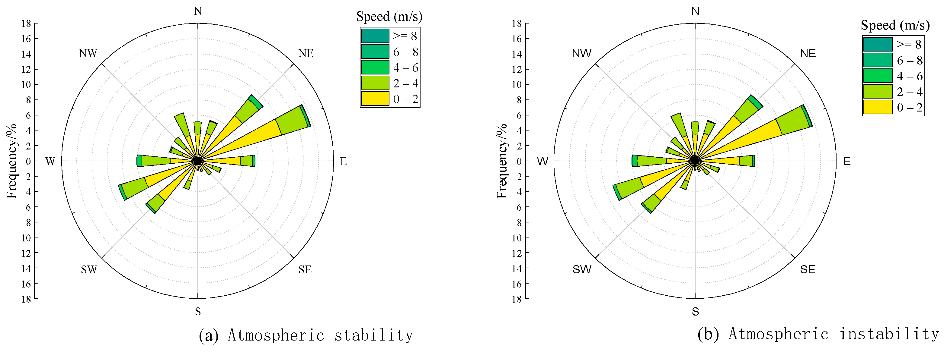
5.1. Wind Direction Characteristics in the Source Region

Using meteorological data from peatlands during the 2017 growing season, this study analyzed the wind direction distribution and wind speed variations in the study area. The wind direction was divided into 16 intervals of 22.5°, with line segments representing the statistical values for each direction to illustrate the wind frequency. The longer the segment, the higher the frequency, forming a wind rose diagram (Figure 1). The results indicated that during the 2017 vegetation growth season, winds from 0 to 90° (northeast wind) were the most frequent (Figure 1). Under stable and unstable atmospheric conditions, the frequencies of northeast winds were 55.7% and 39.7%, respectively. The wind frequency ratios for 90–180°, 180–270°, and 270–360° were 8.3% and 19.4%, 18.2% and 29.6%, and 17.8% and 20.3%, respectively. The maximum wind speed under stable conditions was 6.5 $\mathrm{m}·{\mathrm{s}}^{-1}$, with an average wind speed of 1.2 $\mathrm{m}·{\mathrm{s}}^{-1}$. In contrast, under unstable conditions, the maximum wind speed reached 7.4 $\mathrm{m}·{\mathrm{s}}^{-1}$, with an average wind speed of 1.6 $\mathrm{m}·{\mathrm{s}}^{-1}$ in the prevailing wind direction (

Table 2. Wind direction and speed characteristics under various conditions.

Stability	Wind Direction (°)	Maximum Wind Speed (m·s−1)	Average Wind Speed (m·s−1)	Wind Speed Frequency (%)	Prevailing Wind Direction
L > 0	Northeast (0–90°)	6.1	1.2	55.7%	Northeast-Southwest Wind
	Southeast (90–180°)	6.5	1.2	8.3%
	Southwest (180–270°)	5.3	1.2	18.2%
	Northwest (270–360°)	6.1	1.2	17.8%
L < 0	Northeast (0–90°)	7.4	1.6	39.7%
	Southeast (90–180°)	5.5	1.6	19.4%
	Southwest (180–270°)	5.5	1.6	29.6%
	Northwest (270–360°)	6.2	1.6	20.3%

Note: L > 0 indicates a stable state of the atmosphere, and L < 0 indicates an unstable state of the atmosphere.

).

In 2017, the frequencies of northeast winds during spring, summer, autumn, and the entire growing season were 50.0%, 47.2%, 45.6%, and 46.3%, respectively, whereas the southwest winds accounted for 19.2%, 27.2%, 25.1%, and 24.9%, respectively (

Table 3. Wind direction and frequency at different times.

Time	Frequency/%				Prevailing Wind Direction
	Northeast Wind	Southwest Wind	Southeast Wind	Northwest Wind
Spring	50	19.2	5.8	25	Northeast-Southwest Wind
Summer	47.2	27.2	10.5	15.1
Autumn	45.6	25.1	11.1	18.2
Growing season	46.3	24.9	9.6	19.2

). These results revealed that the primary wind direction in the study area was from northeast to southwest (Figure 2), with other wind directions occurring less frequently. As the wind direction in the source area shifted from northeast to southwest, the footprint distribution of the flux source area and the flux contribution rate of different vegetation types also changed accordingly.

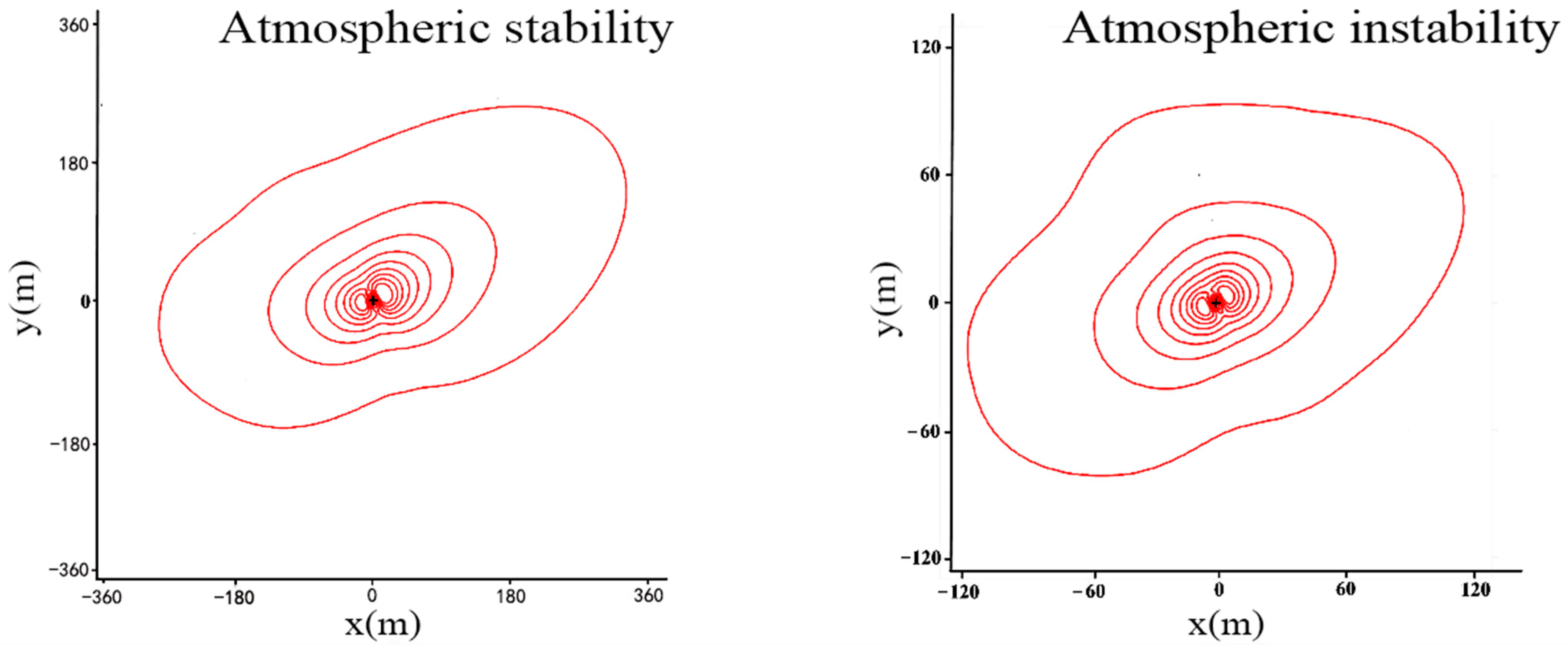
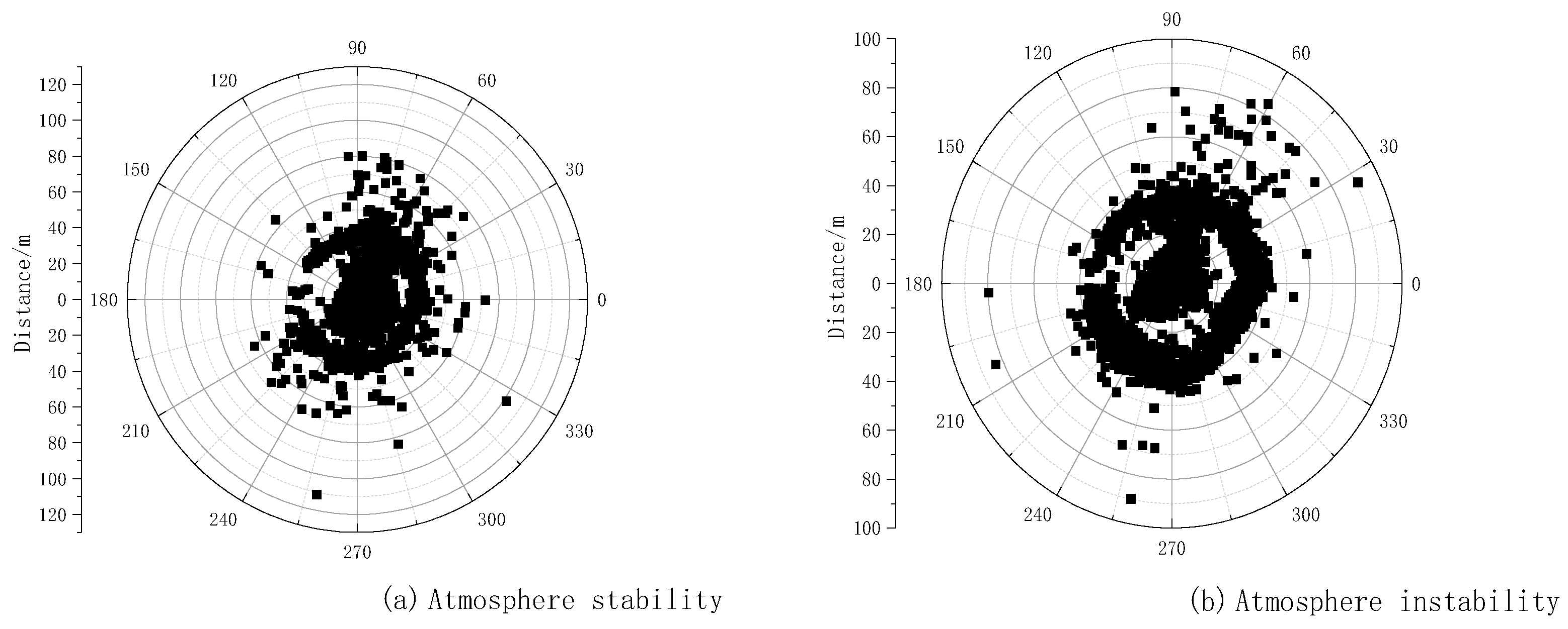
5.2. Overall Distribution Characteristics of Flux Contribution Areas

This study implemented the Kljun model to analyze the 90% flux contribution of the study area under different seasons and atmospheric stability conditions. During the growing season, the flux source region was significantly smaller under unstable atmospheric conditions than under stable conditions (Figure 3). Under unstable conditions, the length range of 90% of the flux contribution area was 61.5–185.6 m, while under stable conditions, it extended from 117.3 to 393.3 m. Under both atmospheric conditions, the maximum length of the source zone was oriented in the northeast direction, which was consistent with the dominant wind.

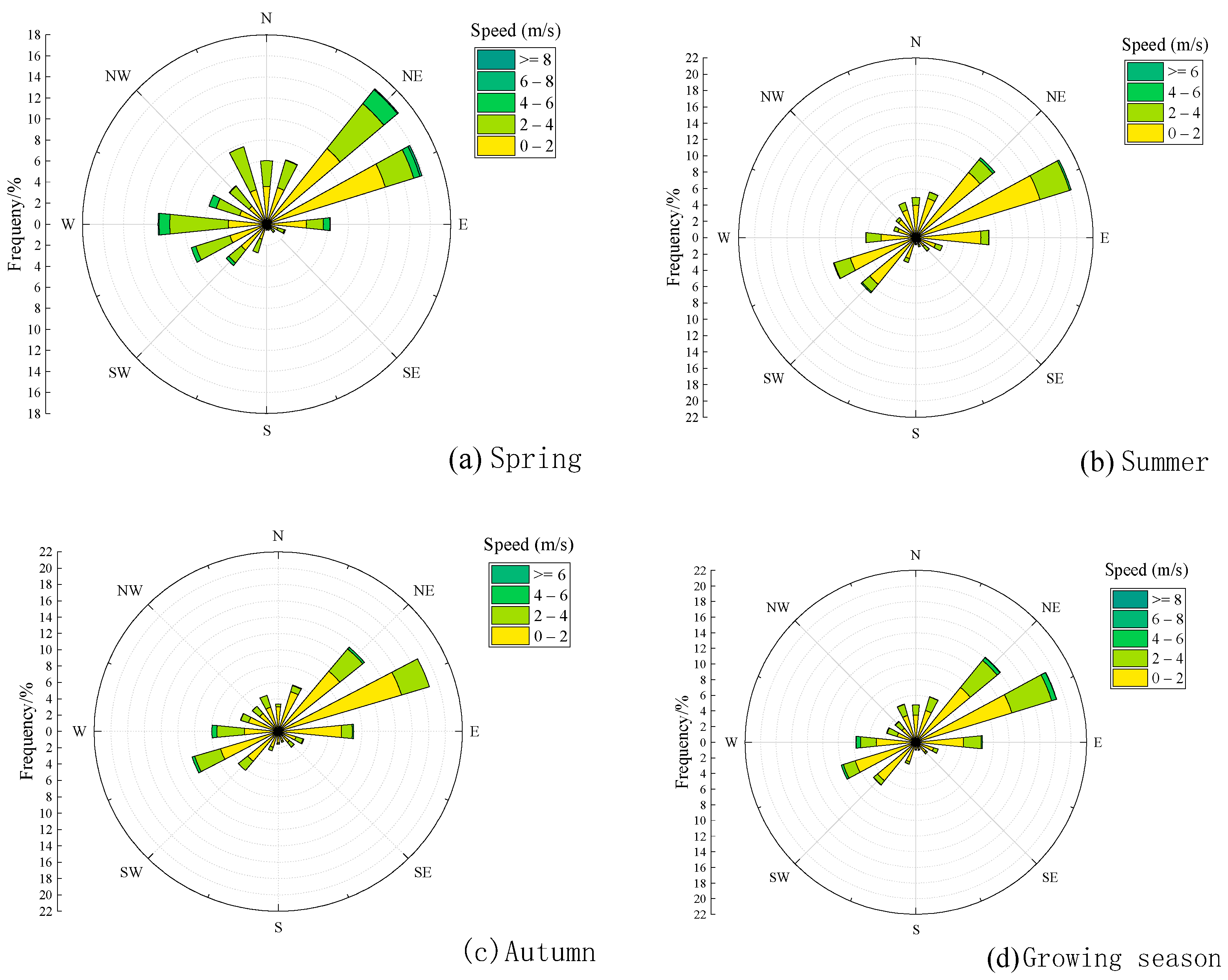
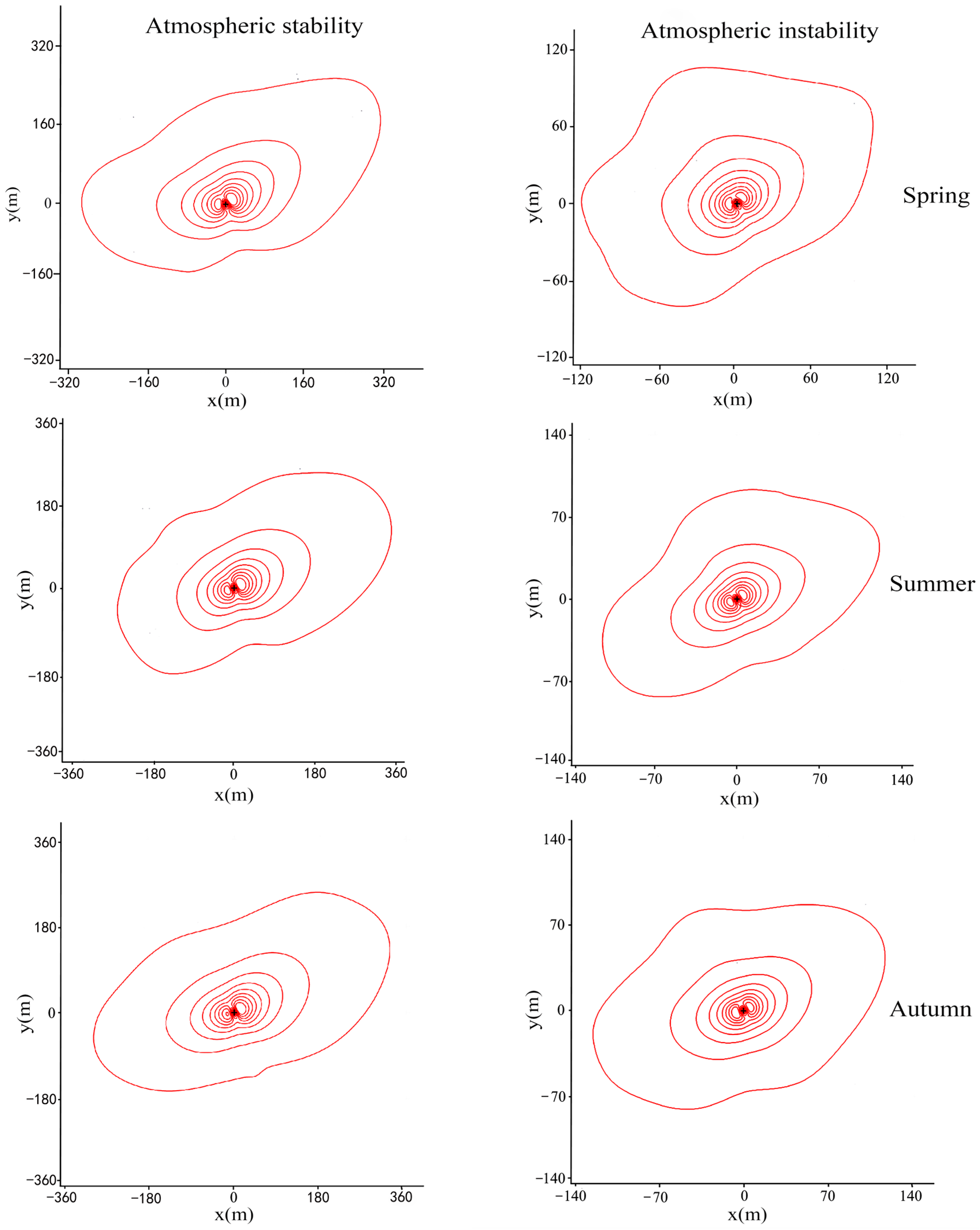
5.3. Seasonal Distribution Characteristics of Flux Contribution Areas

Seasonal differences were observed in the flux contribution areas, with variations in the length and distribution direction of the source area under different seasons and atmospheric stability conditions. Using the Kljun model, this study analyzed the changes in the flux contribution areas of peatlands across different seasons (Figure 4). When the cumulative flux contribution reaches 90%, the length of the source area in the northeast direction during spring ranged from 140.2 to 374.6 m under the stable conditions and 62.4–183.3 m under the unstable conditions, while in the southwest direction, it ranged from 117.5 to 330.2 and 68.3 to 125.1 m, respectively. In summer, the northeast direction extended 122.5–393.3 m under stable conditions and 72.6–185.6 m under unstable conditions, whereas in the southwest direction, it spanned 131.3–320.4 m and 69.4–141.4 m, respectively. During autumn, the northeast direction ranged from 134.9 to 379.8 m under stable conditions and 67.3–184.3 m under unstable conditions, while the southwest direction extended 117.3–337.5 and 67.7–123.2 m, respectively. Across all seasons, the maximum source area length occurred in the 0–90° and 180–270° directions. These results indicated that in summer, the flux contribution areas in the northeast-southwest predominant wind corridor were the largest, with the farthest distances in all seasons aligning with the predominant wind corridor. Additionally, the maximum source area length under stable conditions exceeded that under unstable conditions, which was consistent with the source area distribution characteristics throughout the growing season.

The analysis of the spatial distribution of maximum flux contribution points (Figure 5) revealed that under stable atmospheric conditions, these points were distributed within 111.2 m, with the majority concentrated within 40 m. Under unstable conditions, the maximum flux contribution rate was distributed within 90.7 m, a primarily of 40 m. These findings highlight the importance of minimizing human interference near vorticity towers during flux observations, particularly in natural ecosystems such as wetlands and grasslands in the northern regions.

5.4. Flux Contribution Rates of Different Vegetation Types Within the Source Area

Integrating the spatial distribution of vegetation types within the flux contribution areas and peatlands can provide a more intuitive understanding of the role of vegetation in flux observations. Vegetation coverage was quantified using a grid-based field survey (20 m × 20 m grids). Within each grid, the percent cover of trees, tall shrubs, short shrubs, sedges, and mosses was visually estimated by trained observers. ART Footprint Tool integrates vegetation distribution data (from grid surveys) with flux footprint probabilities to calculate the relative contribution of each vegetation type. Specifically, the contribution of each vegetation type (%) was determined by multiplying its percentage cover within a grid by the flux footprint probability of that grid (i.e., Contribution (%) = Vegetation cover (%) × Footprint probability). Using the ART Footprint Tool [13,26,27], quantitative analysis was performed to assess the cumulative flux contribution of various vegetation types to the flux values within each grid (Figure 6). The results indicated that regardless of season, the contribution proportions of vegetation types within the 90% flux contribution areas remained similar. From the highest to the lowest, they were tall shrubs (28.5–30.3%), short shrubs (27.1–28.8%), sedges (18.6–19.9%), mosses (16.7–17.7%), and trees (0.4–0.6%). Overall, shrubs accounted for the largest proportion (approximately 60%) of the flux contribution areas, while sedges and mosses had comparable influences (16.7–17.7% and 18.6–19.9%, respectively), and trees had the lowest impact (≤0.6%). These findings establish that shrubs played the most significant role in flux observations and the surface carbon budget of peatlands, followed by sedges and mosses, whereas the influence of trees was negligible.

6. Discussion

This study adopted the flux footprint model to analyze the distribution of flux contribution area in typical peatlands of the permafrost region in the Greater Khingan Range across different periods. The results demonstrated that while the primary distribution direction of the peatland flux contribution areas remained unchanged owing to the regional wind direction and speed, the location and size of the source area varied by season. During summer, when the wind direction and speed fluctuated more significantly, the contribution area exhibited higher variability and a wider distribution range compared with other seasons and the flux contribution areas range under stable conditions extended up to 393.3 m (Figure 4), exceeding spring (374.6 m) and autumn (379.8 m), likely due to stronger wind speed variability (Table 2). Furthermore, the flux contribution areas under stable atmospheric conditions were significantly larger than those under unstable conditions (Figure 4). Under stable conditions, the weaker air turbulence and slower vertical diffusion of matter caused the flux signals to originate from areas farther from the observation tower. In contrast, under unstable conditions, the velocity difference between the vertical and horizontal airflows increased, leading to stronger convective mixing and turbulence. Consequently, the flux observations under unstable conditions were influenced more by the surface environmental factors within smaller areas, with the flux signals primarily originating from regions closer to the observation tower, resulting in a smaller contribution area. These findings are consistent with those of previous studies on the distribution of flux observation source areas in broad-leaved Korean pine forests on Changbai Mountain [16] and the temporal variation of carbon flux contribution areas in bamboo forests in Anji County, Zhejiang Province [35].

Atmospheric stratification, observation tower height, and surface roughness can influence the range of the flux-contribution zone. By analyzing the changes in the flux contribution areas, this study provides a better understanding of how peat underground bedding can affect the flux observation results. The vegetation varieties of the underlying surface are not unique, and different types of vegetation are distributed in patches, and the height of the canopy is also different. Under this premise, the heterogeneous underlying surface has a certain influence on the flux. Specifically, the spatial variability of vegetation (e.g., shrubs, sedges, and mosses) modifies surface roughness and gas exchange dynamics, while the peat layer’s depth and composition regulate water retention and carbon storage capacity. These combined effects shape the observed flux signals.

Compared with similar studies on flux contribution areas (

Table 4. Flux source areas under stable atmospheric conditions for different ecosystems.

Ecosystem	Representative Vegetation	Measure Height (m)	P Level (%)	E (m)	References
Forest ecosystem	Mixed conifer and broadleaf forest	40	80	2717	[16]
Forest ecosystem	Phyllostachys pubescens forest	25	90	3500	[35]
Wetland ecosystem	Wetland	14	90	836	[36]
Desert ecosystem	Haloxylon ammodendron	11	90	670.8	[37]
Agro-ecosystem	Zea mays	3	90	155	[38]
Agro-ecosystem	Rice-wheat rotation	4	80	158	[39]
Forest ecosystem	Aspen	37	80	550	[40]
Wetland ecosystem	Phragmites australis	5	90	439	[41]
Agro-ecosystem	Triticum aestivum	3.5	90	222	[42]
Wetland ecosystem	peatland	2.9	90	390	The present research

), the flux contribution areas range in this peatland system was relatively small, with a maximum distance of 393.3 m. This was attributed to certain factors such as the underlying surface, vegetation canopy height, and instrument observation height. In the peatlands dominated by shrubs and herbs, the instrument installation height was relatively low (approximately 3 m). In contrast, the Anji bamboo forest ecosystem, with an instrument height of 25 m, has a maximum source area distance of 3500 m [35]. Different studies have adjusted the instrument installation height based on vegetation height. For example, in forest ecosystems where vegetation reaches tens of meters, instrument placement is adjusted accordingly. This variation in installation height was the primary reason for the differences in source area length across research sites. In the wetland ecosystem at the ninth section of the Yangtze River estuary, with instruments installed at 14 m, the maximum flux contribution distance reaches 836.2 m [36]. In the desert ecosystems of the arid northwestern region, an instrument height of 11 m corresponds to a 90% flux contribution area, reaching 686 m [37]. Similar to this study, agricultural ecosystem research at an observation height of 3 m discovered a 90% flux contribution area extending only 155 m [38]. These findings highlight the significant impact of the observation height on the size of the flux source area in flux observation studies.

The vegetation types on the underlying surface and their spatial distribution can fundamentally influence the investigation of flux contribution areas. The larger the proportion of a vegetation type within the source area, the higher the percentage contribution to the source area (Figure 6). In this study, shrubs accounted for 60% of the peatland area, with their flux contribution being three times that of other vegetation types, such as sedges and mosses. Similar findings have been observed in the mixed coniferous and broad-leaved forests of Fengyang Mountain, where the dominant vegetation (bamboo forest) has a greater impact on the flux contribution areas [23]. Future research, particularly in complex terrain, should prioritize developing and applying source area models that incorporate variations in the underlying terrain and vegetation distribution.

7. Conclusions

This study examined the spatiotemporal distribution characteristics of flux contribution areas and the contributions of different vegetation types in typical peatlands in the permafrost region of the Greater Khingan Range. The following conclusions were drawn.

During the growing season, northeast-southwest winds dominated the study area, with wind frequencies in these directions accounting for 71.2%. Because wind direction was the primary factor influencing the source area distribution, the flux contribution area was aligned with the prevailing wind direction. Under unstable atmospheric conditions, the enhanced vertical airflow mixing rendered the near-ground turbulence more sensitive to surface features within smaller areas, causing the flux observations to originate primarily within 186 m of the observation tower. In contrast, under stable atmospheric conditions, weaker atmospheric motion and turbulence reduced vertical air mixing, resulting in flux signals generated from a larger surface area, approximately 390 m from the observation position.

The distribution of source areas varied by season, with the largest flux contribution range occurring in summer, reaching the maximum distance of approximately 393.3 m, followed by autumn at 379 m, and spring with the smallest maximum distance of about 374 m. In the peatlands of the study area, shrubs, particularly tall shrubs, contributed the most to the flux source area, followed by sedges and moss vegetation, while the influence of scattered trees was negligible.

References

1. Trettin, C.C.; Jurgensen, M.F.; Gale, M.R.; McLaughlin, J.W. Recovery of carbon and nutrient pools in a northern forested wetland 11 years after harvesting and site preparation. For. Ecol. Manag. 2011, 262, 1826–1833. [Google Scholar] [CrossRef]
2. Twine, T.E.; Kustas, W.P.; Norman, J.M.; Cook, D.R.; Houser, P.R.; Meyers, T.P.; Prueger, J.H.; Starks, P.J.; Wesely, M.L. Correcting eddy-covariance flux underestimates over a grassland. Agric. For. Meteorol. 2000, 103, 279–300. [Google Scholar] [CrossRef]
3. Wilson, K.B.; Hanson, P.J.; Mulholland, P.J.; Baldocchi, D.D.; Wullschleger, S.D. A comparison of methods for determining forest evapotranspiration and its components: Sap-flow, soil water budget, eddy covariance and catchment water balance. Agric. For. Meteorol. 2001, 106, 153–168. [Google Scholar] [CrossRef]
4. Grimmond, C.S.B.; King, T.S.; Cropley, F.D.; Nowak, D.J.; Souch, C. Local-scale fluxes of carbon dioxide in urban environments: Methodological challenges and results from Chicago. Environ. Pollut. 2002, 116, S243–S254. [Google Scholar] [CrossRef] [PubMed]
5. Kljun, N.; Calanca, P.; Rotach, M.W.; Schmid, H.P. A simple two-dimensional parameterisation for Flux Footprint Prediction (FFP). Geosci. Model Dev. 2015, 8, 3695–3713. [Google Scholar] [CrossRef]
6. Bao, J.; Zhang, L.; Cao, X.J.; Liang, J.N.; Wang, J. Footprint Analysis for Turbulent Flux Measurements over Complex Terrain on the Loess Plateau of China. Adv. Mater. Res. 2012, 1791, 910–916. [Google Scholar] [CrossRef]
7. Matustik, J.; Koci, V. What is a footprint? A conceptual analysis of environmental footprint indicators. J. Clean. Prod. 2021, 285, 124833. [Google Scholar] [CrossRef]
8. Milanolo, S.; Gabrovšek, F. Estimation of carbon dioxide flux degassing from percolating waters in a karst cave: Case study from Bijambare cave, Bosnia and Herzegovina. Chem. Erde. 2015, 75, 465–474. [Google Scholar] [CrossRef]
9. Mashayek, F.; Pandya, R.V.R. Analytical description of particle/droplet-laden turbulent flows. Prog. Energy Combust. Sci. 2003, 29, 329–378. [Google Scholar] [CrossRef]
10. Vesala, T.; Kljun, N.; Rannik, U.; Rinne, J.; Sogachev, A.; Markkanen, T.; Sabelfeld, K.; Foken, T.; Leclerc, M.Y. Flux and concentration footprint modelling: State of the art. Environ. Pollut. 2008, 152, 653–666. [Google Scholar] [CrossRef]
11. Connan, O.; Maro, D.; Hébert, D.; Solier, L.; Ideas, P.C.; Laguionie, P.; St-Amant, N. In situ measurements of tritium evapotranspiration (3 H-ET) flux over grass and soil using the gradient and eddy covariance experimental methods and the FAO-56 model. J. Environ. Radioact. 2015, 148, 1–9. [Google Scholar] [CrossRef] [PubMed]
12. Schmid, H.P. Footprint modeling for vegetation atmosphere exchange studies: A review and perspective. Agric. For. Meteorol. 2002, 113, 159–183. [Google Scholar] [CrossRef]
13. Kormann, R.; Meixner, F.X. An Analytical Footprint Model for Non-Neutral Stratification. Bound.-Layer Meteorol. 2001, 99, 207–224. [Google Scholar] [CrossRef]
14. Cai, X.; Leclerc, M.Y. Forward-in-time and Backward-in-time Dispersion in the Convective Boundary Layer: The Concentration Footprint. Bound.-Layer Meteorol. 2007, 123, 201–218. [Google Scholar] [CrossRef]
15. Macalkova, L.; Havrankova, K.; Pavelka, M. Flux footprints in different ecosystems. Glob. ChanGe A Complex ChallenGe 2015, 54, 54–57. [Google Scholar]
16. Zhao, X.S.; Guan, D.X.; Wu, J.L.; Jin, C.J.; Han, S.J. Distribution of footprint and flux source area of the mixed forest of broad-leaved and Korean pine in Changbai Mountain. J. Beijing For. Univ. 2005, 27, 17–23. [Google Scholar]
17. Rebmann, C.; Göckede, M.; Foken, T.; Aubinet, M.; Aurela, M.; Berbigier, P.; Bernhofer, C.; Buchmann, N.; Carrara, A.; Cescatti, A.; et al. Quality analysis applied on eddy covariance measurements at complex forest sites using footprint modelling. Theor. Appl. Climatol. 2005, 80, 121–141. [Google Scholar] [CrossRef]
18. Rogiers, N.; Eugster, W.; Furger, M.; Siegwolf, R. Effect of land management on ecosystem carbon fluxes at a subalpine grassland site in the Swiss Alps. Theor. Appl. Climatol. 2005, 80, 187–203. [Google Scholar] [CrossRef]
19. Hutjes, R.W.A.; Vellinga, U.S.; Gioli, B.; Miglietta, F. Dis-aggregation of airborne flux measurements using footprint analysis. Agric. For. Meteorol. 2010, 150, 966–983. [Google Scholar] [CrossRef]
20. Kim, J.; Hwang, T.; Schaaf, C.L.; Kljun, N.; Munger, J.W. Seasonal variation of source contributions to eddy-covariance CO2 measurements in a mixed hardwood-conifer forest. Agric. For. Meteorol. 2018, 253, 71–83. [Google Scholar] [CrossRef]
21. Sun, S.; Wang, W.; Xu, F. Comparison of Footprint Models of Surface Heat and Water Vapor Fluxes in the Middle and Upper Reaches of Heihe River Basin. Remote Sens. Technol. Appl. 2021, 36, 887–897. [Google Scholar]
22. Zhang, H.; Wen, X. Flux Footprint Climatology Estimated by Three Analytical Models over a Subtropical Coniferous Plantation in Southeast China. J. Meteorol. Res. 2015, 29, 654–666. [Google Scholar] [CrossRef]
23. Ji, X.; Gong, Y.; Zheng, X.; Lu, J.; Feng, M.; Zhuang, J.; Ye, L.; Liu, S.; Fang, W.; Wang, D.; et al. Distribution and characteristics of flux footprint of coniferous and broad-leaved mixed forest ecosystem in Fengyang Mountain of Zhejiang, China. Acta Ecol. Sin. 2020, 40, 7377–7388. [Google Scholar]
24. Wang, X.; Song, C.; Chen, N.; Qiao, T.; Wang, S.; Jiang, J.; Du, Y. Gas storage of peat in autumn and early winter in permafrost peatland. Sci. Total Environ. 2023, 898, 165548. [Google Scholar] [CrossRef] [PubMed]
25. Miao, Y.; Song, C.; Sun, L.; Wang, X.; Meng, H.; Mao, R. Growing season methane emission from a boreal peatland in the continuous permafrost zone of Northeast China: Effects of active layer depth and vegetation. Biogeosciences 2012, 9, 4455–4464. [Google Scholar] [CrossRef]
26. Shi, F.X.; Wang, X.W.; Lin, G.G.; Zhang, X.H.; Chen, H.M.; Mao, R. Cryptogams and dwarf evergreen shrubs are vulnerable to nitrogen addition in a boreal permafrost peatland of Northeast China. Appl. Veg. Sci. 2022, 25, e12691. [Google Scholar] [CrossRef]
27. Liu, S.M.; Xu, Z.W.; Wang, W.; Jia, Z.Z.; Zhu, M.J.; Bai, J.; Wang, J.M. A comparison of eddy-covariance and large aperture scintillometer measurements with respect to the energy balance closure problem. Hydrol. Earth Syst. Sci. 2011, 15, 1291–1306. [Google Scholar] [CrossRef]
28. Berry, Z.; Smith, W. Cloud pattern and water relations in Picea rubens and Abies fraseri, southern Appalachian Mountains, USA. Agric. For. Meteorol. 2012, 162, 27–34. [Google Scholar] [CrossRef]
29. Webb, E.; Pearman, G.; Leuning, R. Correction of flux measurements for density effects due to heat and water vapour transfer. Q. J. R. Meteorol. Soc. 1980, 106, 85–100. [Google Scholar] [CrossRef]
30. Moncrieff, J.; Massheder, J.; de Bruin, H.; Elbers, J.; Friborg, T. A system to measure surface fluxes of momentum, sensible heat, water vapour and carbon dioxide. J. Hydrol. 1997, 188, 589–611. [Google Scholar] [CrossRef]
31. Mauder, M.; Foken, T. Quality control of eddy covariance data based on a classification system for flux measurement sites. Theor. Appl. Climatol. 2004, 80, 81–92. [Google Scholar]
32. Schmid, H.P. Experimental design for flux measurements: Matching scales of observations and fluxes. Agric. For. Meteorol. 1997, 87, 179–200. [Google Scholar] [CrossRef]
33. Kljun, N.; Rotach, M.W.; Schmid, H.P. A Three-Dimensional Backward Lagrangian Footprint Model For A Wide Range Of Boundary-Layer Stratifications. Bound.-Layer Meteorol. 2002, 103, 205–226. [Google Scholar] [CrossRef]
34. Kljun, N.; Kormann, R.; Rotach, M.W.; Meixer, F.X. Comparison of the Langrangian footprint model LPDM-B with an analytical footprint model. Bound.-Layer Meteorol. 2003, 106, 349–355. [Google Scholar] [CrossRef]
35. Zhang, K.D.; Yao, J.; Ling, X.F.; Yan, S.W.; Zhang, F.M.; Lu, Y.Y. Distribution characteristics of flux source of rice-wheat rotation agroecosystem in Huaihe River Basin. Chin. J. Ecol. 2023, 43, 3113–3120. [Google Scholar]
36. Gong, X.F.; Chen, L.P.; Mo, L.F. Research of Flux footprint of Anji Bamboo forest ecosystems based on the FSAM Model. J. Southwest For. Univ. 2015, 35, 37–44. [Google Scholar]
37. Wu, D.X.; Li, G.D.; Zhang, X. Flux footprint of winter wheat farmland ecosystem in the North China Plain. Chin. J. Appl. Ecol. 2016, 28, 3663–3674. [Google Scholar]
38. Chen, Z.H.; Huang, Y.; Tang, J.W.; Tian, B.; Shen, F.; Wu, P.F.; Yaun, Q.; Zhou, C.; Wang, J.T. Flux footprint analysis of a salt marsh ecosystem in the Jiuduansha Shoals of the Changjiang Estuary. J. East China Norm. Univ. 2021, 2, 42–53. [Google Scholar]
39. Zhou, Q.; Li, P.H.; Wang, Q.; Zheng, C.L.; Xu, L. A footprint analysis on a desert ecosystem in west China. J. Desert Res. 2014, 34, 98–107. [Google Scholar]
40. Jin, Y.; Zhang, Z.Q.; Fang, X.R.; Kang, M.C.; Cha, T.G.; Wang, X.P.; Chen, J.Q. Footprint analysis of turbulent flux over a poplar plantation in Northern China. Acta Ecol. Sin. 2011, 32, 3966–3974. [Google Scholar]
41. Gu, Y.J.; Gao, Y.; Guo, H.Q.; Zhao, B. Footprint analysis for carbon Flux in the wetland ecosystem of Chongming Dongtan. J. Fudan Univ. 2008, 3, 374–379+386. [Google Scholar]
42. Dong, J.; Dang, H.H.; Kong, F.L.; Yue, N.; Wang, G.; Guo, Y.; Wei, G.X. Analysis of agro-ecosystem footprint of flux in semi-arid areas. Chin. J. Eco-Agric. 2015, 23, 1571–1579. [Google Scholar]
Figure 1. Wind rose map under different atmospheric conditions during the observation period in 2017.
Atmosphere 16 00452 g001
Figure 2. Wind rose map of the study area.
Atmosphere 16 00452 g002
Figure 3. Distribution of source regions under different stability conditions. Note: (0,0) points are observation points, and the east-west directions are the positive and negative directions of the x-axis, respectively. The north and south directions are the negative and positive y-axis directions, respectively. The same convention was applied throughout.
Atmosphere 16 00452 g003
Figure 4. Flux footprints for different seasons. (The vorticity correlation tower is the point (0,0) in the coordinate system with the positive direction of the x axis to the east and the positive direction of the y axis to the north).
Atmosphere 16 00452 g004
Figure 5. Distribution of the flux footprint furthest point.
Atmosphere 16 00452 g005
Figure 6. Proportion of source area contribution by vegetable type.
Atmosphere 16 00452 g006