Revealing Vertical Distribution of Atmospheric Mercury Using Drone-Based Monitoring Technique: A Case Study in Vietnam

Abstract

Unmanned aerial vehicles (UAVs) have emerged as effective tools for monitoring air pollution across varying altitudes, including assessing atmospheric mercury (Hg) levels. However, studies on the vertical distribution of atmospheric Hg (i.e., total gaseous mercury–TGM) concentrations remain limited, particularly in Southeast Asia. This study utilized a UAV equipped with a TGM sampling device to measure concentrations at different altitudes in Ben Cat City, an industrial area in Southern Vietnam. The purpose of this study is to examine the applicability of UAV in investigating the altitudinal distribution of TGM and to analyze specific case studies related to Hg emissions from stack. A total of 36 flight experiments were conducted (including 36 concurrently ground level measurements), including 50 m (20 flights), 200 m (7 flights), and 500 m (9 flights). TGM concentrations increase noticeably with altitude under stack emission conditions, while they remain relatively consistent at all altitudes during non-emission conditions. Under the emission conditions, three vertical distribution patterns were observed: (1) elevated TGM concentrations at higher altitudes compared to ground level; (2) lower TGM concentrations at higher altitudes relative to ground level; and (3) nearly equivalent TGM concentrations between ground level and higher altitudes, with differences less than 0.4 ng m⁻³. The observed distributions imply the important role of atmospheric dynamics in understanding the dispersion of pollutants and the impact of emissions. This study pioneers the use of UAVs in Vietnam for simultaneous TGM measurements across altitudes, highlights their potential for atmospheric Hg monitoring, and improves stack emission management.

1. Introduction

Mercury (Hg) has long been recognized as a global pollutant with high toxicity, bioaccumulation potential, and significant risks to public health and the environment [1,2,3,4]. Atmospheric Hg predominantly exists as gaseous elemental mercury (GEM), gaseous oxidized mercury (GOM), and particulate-bound mercury (PBM), with total gaseous mercury (TGM = GEM + GOM) comprising over 95% of its total abundance [4,5,6]. Notably, Hg is a key indicator for pollution driven by anthropogenic activities, with stack emission as a primary source [4,7]. Fossil fuel combustion in industrial processes is a major source of atmospheric Hg, yet its vertical transport and distribution remain poorly understood. Monitoring vertical Hg profiles is essential for determining the altitude and transport of pollutants, thus directly influencing its environmental impact on surrounding regions [8,9,10]. These profiles provide critical insights into dispersion mechanisms, supporting environmental assessments and the development of effective pollution-control strategies.

Unmanned aerial vehicles (UAVs) are equipped with mobile atmospheric observation systems to monitor airborne pollutants. The improvements in the design of UAVs offer several advantages compared to the traditional monitor, including the flight stability, adjustable flight speeds, and flexible flight paths [11,12,13]. For instance, Li et al., 2022 employed multirotor UAVs equipped with mobile air pollution sensors to investigate the three-dimensional distribution of traffic-related pollutants in Shanghai [12]. The results showed a 44% reduction in PM₁ concentration near high-rise buildings, highlighting the superior spatial resolution of UAVs compared to traditional methods, such as satellite remote sensing, meteorological balloons, and fixed-wing drones. For Hg studies using UAVs, Salgado et al., 2023 applied UAV-RS and Random Forest algorithm to map Hg and As in contaminated areas, achieving greater accuracy, especially in vegetation [14]. However, this study primarily focused on surface mapping and lack of exploration of the vertical distribution of pollutant concentrations. A recent study by Cabassi et al., 2022 employed a UAV–Lumex system to measure GEM at an Hg mining site in Italy [15]. The study demonstrated the system’s high sensitivity, which is advantageous for detecting GEM concentrations. However, the measurements were only conducted at determined altitudes, without the record of the ground level’s concentration. The lack of ground-level data constrains the ability to comprehensively assess the vertical distribution of GEM within the study area. Although UAVs have been employed in various studies for air pollution monitoring, including Hg measurements, the number of such investigations remains relatively limited. This limitation is primarily due to persistent technical challenges, such as lack of consistent data across different heights and environmental conditions, and the need for further refinement in the integration of UAV systems with ground-based monitoring tools.

This study was conducted with the advancements in UAV technology, marking the first application of a custom-designed multirotor UAV in Vietnam for TGM sampling. The study pursued two key objectives: (1) to investigate the variation in TGM concentrations at ground level and different altitudes using UAV; and (2) to assess the influence of emission conditions on TGM concentrations. Our study provides preliminary insights into the TGM vertical distribution and highlights the potential of using UAV technology for air quality monitoring. Additionally, it offers essential baseline data that will support future research and developing strategies for air quality management in Vietnam. However, we acknowledge that a comprehensive understanding and precise evaluation of the factors influencing the altitudinal distribution of TGM are beyond the scope of this study.

2. Materials and Methods

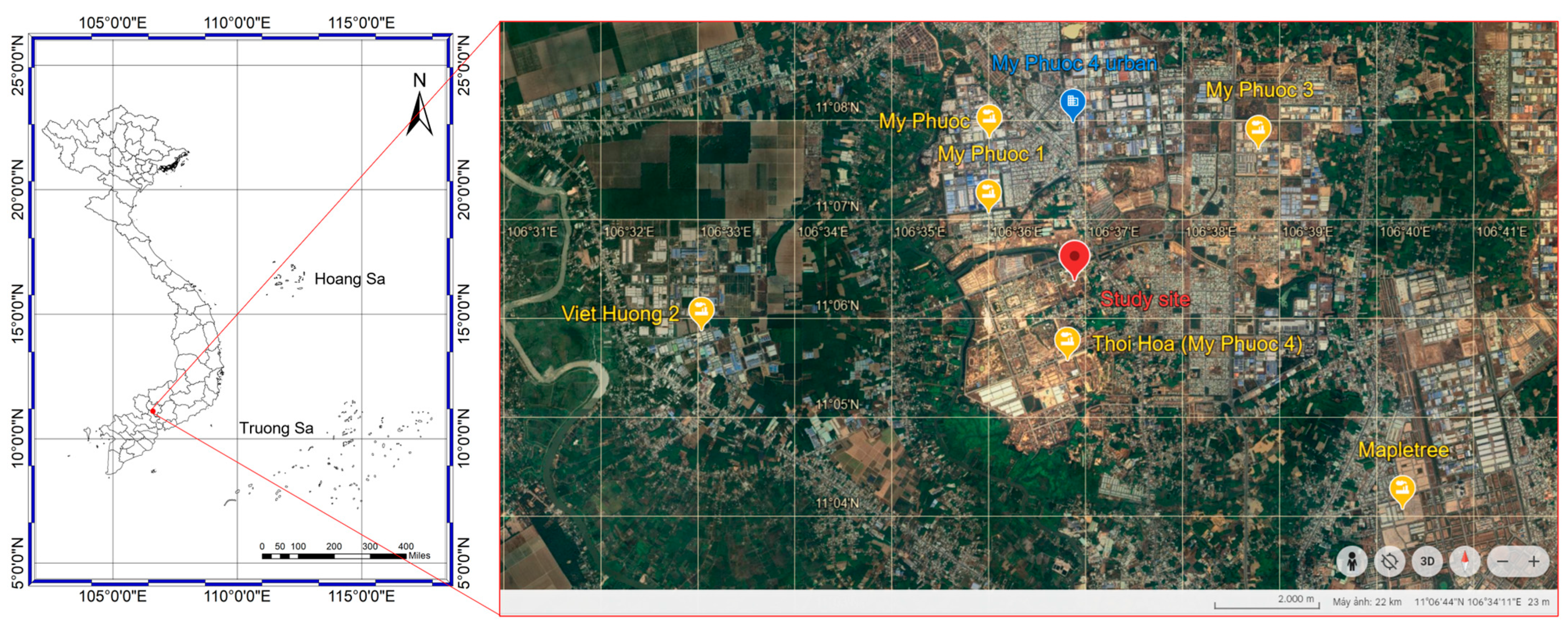
2.1. Research Location

This research was conducted at the Vietnamese–German University (VGU; 11.10° N, 106.61° E), situated in Ben Cat City, Binh Duong Province, an emerging industrial hub in Southern Vietnam, characterized by its proximity to multiple industrial zones within a 10 km radius with complex industrial activities. All flight operations were conducted within the sports field of the university (Figure 1). Specifically, the research site lies approximately 8 km west of Viet Huong 2 Industrial Park, 2 km from My Phuoc 1, 3 km northwest of My Phuoc, about 4 km from My Phuoc 3, 7.5 km southeast of the Mapletree Industrial Zone, and 1.5 km from Thoi Hoa (My Phuoc 4) Industrial Park (Figure 1). Additionally, the My Phuoc 4 urban area is located roughly 3 km to the north and within a 1 km radius, and the area surrounding the site is influenced by the activities of small-scale enterprises. Notably, three emission sources (stacks) have been identified, originating from stacks of facilities engaged in garment manufacturing, packaging production, and plywood processing. The heights of these stacks are estimated at about 15–20 m, varying according to the specific operational processes and the scale of each establishment. These stacks represent important sources of air pollution in close proximity to the observation site and have the potential to significantly influence the local environment. However, the emission rates from these sources were not directly measured in this study. Such measurements were beyond the scope of the present study, which primarily focused on UAV-based vertical Hg profiling.

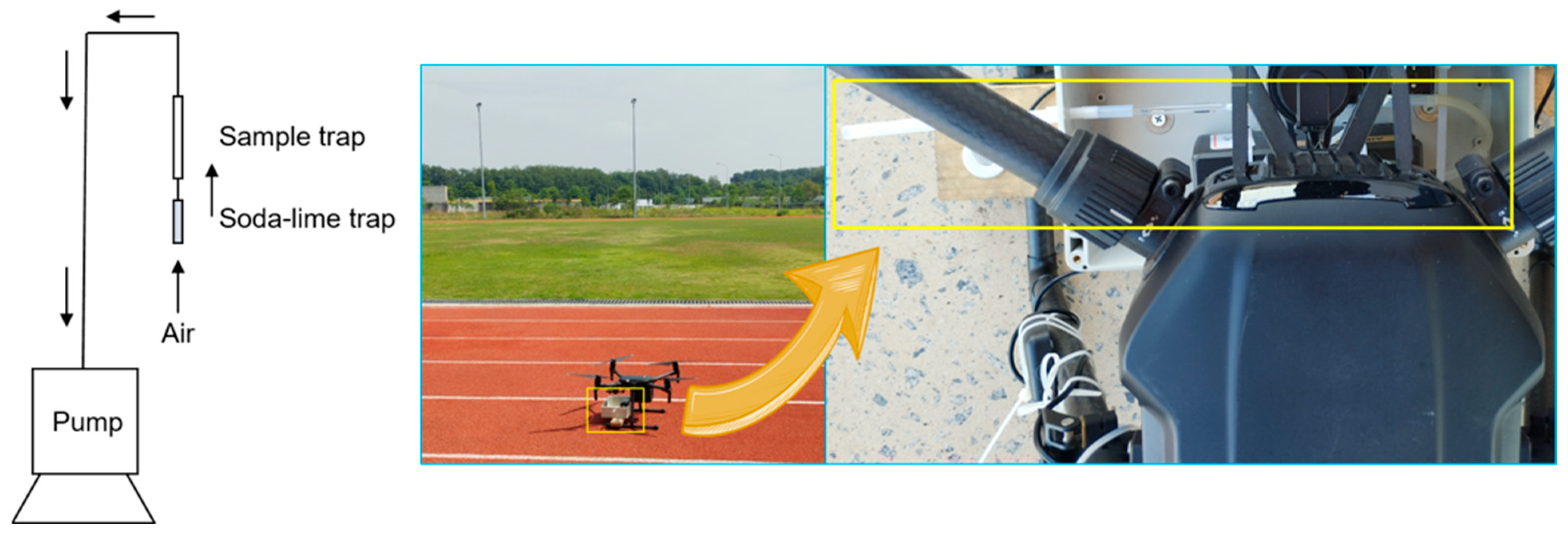
2.2. TGM Sampling Using UAV

A manual active sampling method for TGM following the US EPA’s IO-5 protocol was used in this study. The detection limit of the NIC WA-5F system used in this study is approximately 5 pg Hg, ensuring high sensitivity for atmospheric Hg analysis. It should be noted that the average concentration of all samples was significantly above the detection limit, with values exceeding 40 pg Hg, confirming the reliability of the measurements. The measurement uncertainty was evaluated through parallel sampling and comparison with the Tekran 2600, showing an average deviation of less than 10%, which complies with the quality standards of major global Hg monitoring networks [16]. A manual active sampling method for TGM following the US EPA’s IO-5 protocol was used in this study. This approach, extensively examined in previous studies [2,9,17] substantiates its robustness and reliability for sample collection and analytical procedures. TGM was sampled using a system comprising a gold trap (NIC, Japan) preceded by a 7 cm soda-lime trap to remove PBM, ensuring accurate measurement of TGM (Figure 2—[2,17]). Ambient air was drawn through the gold trap (1 L min⁻¹) using an SKC AirChek 52 pump (SKC, USA). Upon completion of the sampling process, the gold traps were placed in specialized glass tubes, sealed with two layers of ziplock bags, and transported to the laboratory for analysis. Blank samples were prepared and analyzed alongside field samples to monitor potential contamination and verify the reliability of the sampling and handling procedures. The SKC pump was calibrated using the Defender 510 device prior to each flight. To ensure data integrity, traps were handled with gloves to prevent contamination, and collected samples were stored securely in sealed glass tubes (Nippon Instruments Corporation, Kyoto, Japan) within double ziplock bags. All blank samples showed concentrations lower than the method detection limit (MDL) of ~4 pg Hg, demonstrating minimal contamination.

A DJI Matrice 200 UAV was employed to carry a TGM sampling device for this study. Due to DJI’s safety-imposed flight height limit of 500 m, observations were conducted between 50 m and 500 m above ground [18,19]. The UAV and its payload demonstrated reliable performance, ensuring data accuracy. This multirotor UAV, weighing 4.53 kg, with dimensions of 887 × 880 × 378 mm, supported a payload of up to 1.61 kg, comfortably accommodating the ~0.5 kg sampling device. With a maximum ascent speed of 5 m s⁻¹, it was equipped with a navigation system, GPS receiver, inertial sensors, and distance sensors [19,20,21]. In P-mode with a stable GPS signal and the Downward Vision System (DVS), the UAV achieved positional accuracy of ±0.1–0.5 m vertically and ±0.3–1.5 m horizontally, ensuring precise sampling locations. Before each flight, the UAV’s sampling system, including the specially designed sampling box, was carefully inspected and calibrated to ensure precise weight balance. This calibration process was conducted through specialized UAV-control software. It controls the balance of the UAV and the sampling device, ensuring that they remain horizontally aligned and free from tilt.

The maximum flight duration of the UAV was 15–20 min with an RGB camera and approximately 15 min with a TIR camera, reflecting the higher energy demands of thermal imaging, but the average flight time in this study was limited to an appropriate 15 min due to battery constraints. The total flight duration was divided into specific segments based on altitude. For example, ascending to a target altitude of 500 m took longer than reaching 50 m. Sampling was initiated at ground level and at each target altitude as soon as the flight began, and it continued until the controlled landing. The pump was turned off immediately after landing, and the sampling time was recorded. Typically, 1–2 min was spent ascending to the target altitude, followed by 8–10 min of sampling at the desired elevation, with an additional 1–2 min allocated for the controlled descent and landing. During experiments involving emission plumes, sampling commenced 3 min after the plume was first detected from the stacks. It is important to note that neither the emission method nor the discharge volume from the stacks was controlled in this study. Emissions occurred in distinct phases dictated by the production process, with durations ranging from approximately 10 to 15 min. Experiments were conducted at a single site, with a consistent flight path for comparability. In addition, based on prior studies, the UAV operated at a speed of 1–3 m s⁻¹ to ensure stable air pollutant sampling [22,23]. Ascent and descent speeds were optimized at 2 m s⁻¹ to conserve battery life and maintain safety. However, to optimize the flight time and improve the efficiency of the sampling process at 500 m, the UAV’s flight speed was increased to 4 m s⁻¹ during flights at this altitude. For each flight, ground-level sampling was performed simultaneously to support comparative analysis. The sampling pump was activated immediately after the UAV took off. Sampling was conducted at 1.5 m above ground level, with UAV and ground samplings synchronized at a consistent flow rate of 1 L min⁻¹ [2,17].

2.3. Hg Analysis

Hg samples were analyzed using the WA-5F [2,9] instrument, which employed a two-step desorption and amalgamation technique (DSGA) combined with an atomic fluorescence spectrometer (AFS) detector. During analysis, the gold traps (samples) were placed in the TC-WA automatic sample changer in sequence. At the start of the analysis, the heater in the TC-WA heated up to 600 °C, releasing all adsorbed Hg as Hg(0), which was then captured by a second gold trap in the WA-5F. Subsequently, the second gold trap was heated and released Hg vapor, moving towards the AFS detector. Hg was measured at a wavelength of 253.7 nm [2,16,24]. For quality assurance, a calibration curve of Hg(0) was created before sample analysis, using the MB-1 NIC Hg(0) vapor generator with varying volumes from 1 to 100 µL (7 points), corresponding to Hg amounts ranging from 0.02 to 2.5 ng. Calibration curves with R² values > 0.9999 and an average deviation in response factor (RF = signal/ng Hg) between points < 3% were used to calculate sample concentration values [1,25]. The study applied the Mann–Whitney U test to compare TGM concentrations at ground level and different altitudes, with the significance level (α) set at 0.05 [26,27]. This test aimed to identify potential differences between sampling locations, thereby providing a scientific basis for further analysis of the vertical distribution of TGM in the atmosphere.

3. Results and Discussion

3.1. TGM Data

A total of 36 pairs of TGM samples (36 flights). The overall mean TGM concentrations (±S.D.) were recorded as 3.09 ± 0.63 ng m⁻³ (range: 2.25–4.91 ng m⁻³) at ground level and 2.99 ± 0.86 ng m⁻³ (range: 1.91–5.13 ng m⁻³) at higher altitudes. The findings revealed that TGM concentrations at ground level 3.02 ± 0.56 ng m⁻³ (range: 2.48–4.91 ng m⁻³) were marginally higher (p < 0.05) than those recorded at 50 m altitude 2.81 ± 0.86 ng m⁻³ (range: 1.91–5.13 ng m⁻³). At an altitude of 200 m, seven flights were conducted, and TGM concentrations at ground level 3.14 ± 0.87 ng m⁻³ (range: 2.25–4.84 ng m⁻³) were slightly lower than those at 200 m altitude 3.43 ± 1.05 ng m⁻³ (range: 1.95–4.90 ng m⁻³). At an altitude of 500 m, 9 flights were conducted, and the results showed that TGM concentrations at ground level 3.21 ± 0.61 ng m⁻³ (range: 2.40–4.07 ng m⁻³) were statistically insignificant (p > 0.05) compared to those at 500 m altitude 3.04 ± 0.66 ng m⁻³ (range: 2.07–4.15 ng m⁻³). Several factors, including meteorological dynamics, emission sources, and atmospheric dilution, could play roles in shaping the vertical distribution of TGM concentrations [28,29]. The results of this study indicate that TGM concentrations were relatively uniform along the vertical profile from the ground up to 500 m above ground level (a.g.l.). This pattern is attributed to two key factors: (1) the measurement site was located in an open field, allowing efficient air circulation and promoting the uniform dispersion of pollutants; and (2) flight experiments were conducted between 9:00 AM and 4:00 PM local time, a period during which the surface boundary layer in the study area was typically stable and extends well beyond 500 m [2,3], facilitating vertical mixing and an even distribution of pollutants. However, it is important to note that this study involved simultaneous measurements under two distinct conditions, the inclusion and exclusion of stack emissions. Therefore, the influence of emissions on the observed data will be analyzed in greater detail in the following sections.

The average TGM concentration at ground level in Ben Cat, Binh Duong (this study), was 3.09 ± 0.63 ng m⁻³, indicating a moderate level of Hg pollution compared to previous studies conducted in urban and suburban areas worldwide. Compared to other urban areas (

Table 1. Comparison of TGM concentrations (ng m⁻³) in urban and suburban areas from different studies worldwide.

Site	Type	Year	TGM (ng m−3)	Reference
Ben Cat, Binh Duong	Urban	2025	3.09 ± 0.63	This study
Ho Chi Minh, Vietnam	Urban	2024	2.49 ± 0.86	[2]
Chennai, India	Urban	2022	4.66 ± 8.35	[34]
Kathmandu, Nepal	Urban	2019	9.9 ± 10.0	[32]
Ulsan, South Korea	Urban	2020–2021	6.89	[33]
Mengzi, China	Urban	2017–2018	2.1 ± 3.5	[30]
Kaohsiung, Taiwan	Urban	2010	6.7 ± 1.4	[35]
Detroit, The United States of America	Urban	2004	2.5 ± 1.4	[31]
Ho Chi Minh, Vietnam	Suburban	2024	1.76 ± 0.50	[2]
Tai Mo Shan, Hong Kong	Suburban	2017	2.26 ± 0.64	[37]
Col Margherita Observatory, Italy	Suburban	2018–2019	3.14 ± 1.29	[36]

), the TGM concentration in Ben Cat was significantly higher than in Ho Chi Minh City, 2.49 ± 0.86 ng m⁻³ [2]; Mengzi, China, 2.10 ± 3.50 ng m⁻³ [30]; and Detroit, USA, 2.50 ± 1.40 ng m⁻³ [31]. The difference results from the proximity of the study area to large industrial zones, contributing to the elevated TGM levels in Ben Cat. Although both Ho Chi Minh City and Ben Cat are located in Southern Vietnam, industrial activities in Ben Cat are more concentrated, releasing more pollutants into the atmosphere. However, the TGM levels in our study were lower than in highly industrialized and polluted cities, such as Kathmandu, Nepal, 9.90 ± 10.00 ng m⁻³ [32]; Ulsan, South Korea, 6.89 ± 0.00 ng m⁻³ [33]; Chennai, India, 4.66 ± 8.35 ng m⁻³ [34]; and Kaohsiung, Taiwan, 6.70 ± 1.40 ng m⁻³ [35]. This suggests that while Ben Cat has higher TGM levels compared to some urban areas, its levels remain lower than in highly industrialized cities. The difference is due to the intensity of industrial activity in cities like Kathmandu, Ulsan, Chennai, and Kaohsiung, resulting in a higher mercury concentration in the atmosphere. In suburban areas, the TGM concentration in Ben Cat is comparable to the levels recorded at Col Margherita Observatory, Italy, 3.14 ± 1.29 ng m⁻³ [36], but it is 1.37 to 1.76 times higher than in Tai Mo Shan, Hong Kong [37], and the suburban region of Ho Chi Minh City [2]. Overall, industrial activities play a significant role in the elevated TGM concentrations at the study sites.

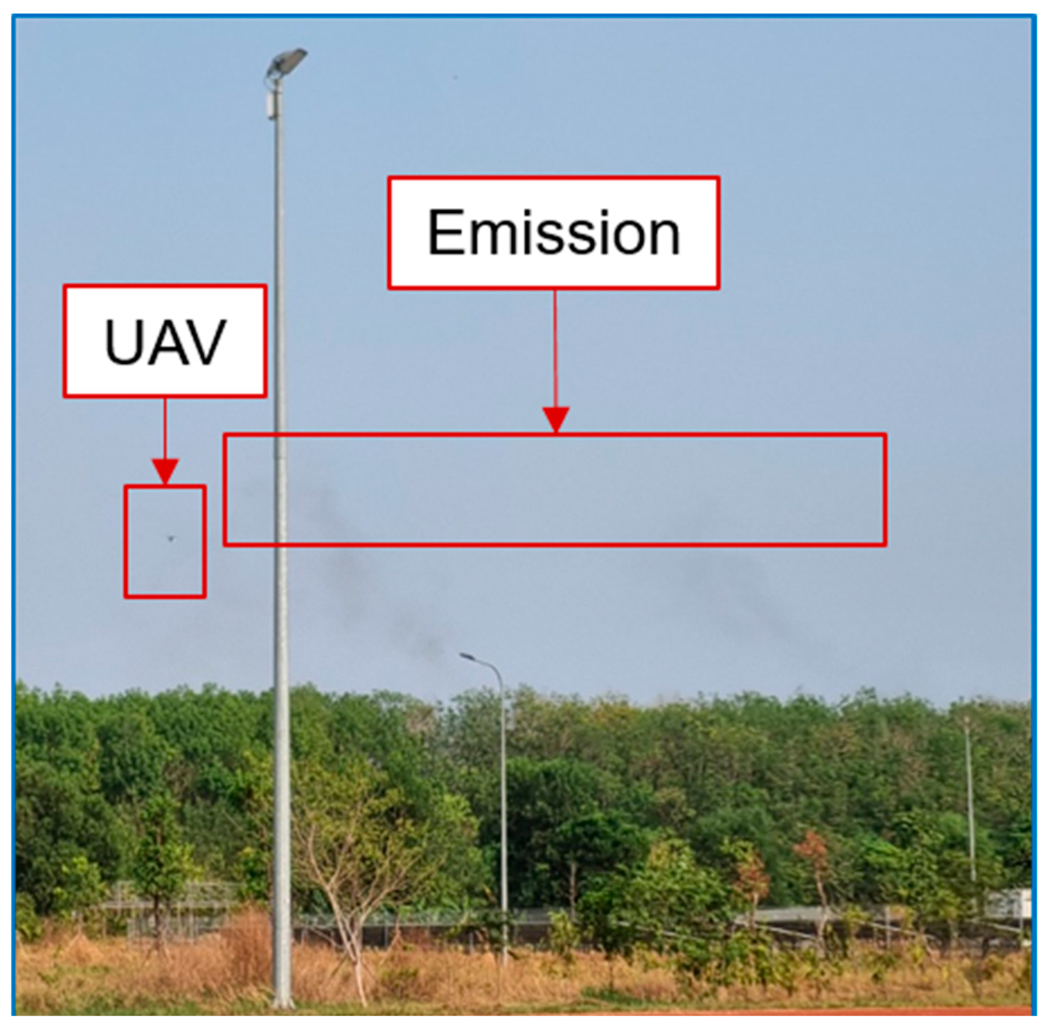
3.2. Distribution of TGM Concentrations Under Normal and Emission Conditions

Figure 3 shows box plots illustrating the variation in TGM concentrations at altitudes of 50 m, 200 m, and 500 m under two distinct conditions (normal and emission conditions), and Figure 4 illustrates the measurement using UAV under the emission condition, as well as showing the emission from stacks. These visualizations provide insights into the vertical distribution of TGM and the extent of influence of the emission source. Under normal conditions (Figure 3a), TGM concentrations remain relatively stable. TGM concentrations showed relatively high S.D. values at ground level, suggesting considerable variability at this height. At 50 m, the mean TGM concentration slightly decreased to 2.78 ± 0.84 ng m⁻³, in the range of 2.12–5.13 ng m⁻³, with a smaller S.D. (0.84), suggesting lower variability compared to ground level. At 200 m, the mean TGM concentration was 3.14 ± 1.00 ng m⁻³, in the range of 1.95–4.46 ng m⁻³; and at 500 m, it was 3.04 ± 0.66 ng m⁻³, in the range of 2.07–4.15 ng m⁻³. The greater S.D. at 200 m compared to 500 m suggests higher fluctuations in TGM concentrations at this intermediate altitude. Further up, at 200 m and 500 m, TGM concentrations continue to decline, with the 500 m level showing the lowest mean value and the narrowest spread among all altitudes. This trend suggests that TGM sources are primarily located near the surface, likely influenced by local emissions, deposition, and atmospheric mixing processes [13,38]. The decreasing concentration with altitude is consistent with previous studies on atmospheric Hg dispersion, thus highlighting the role of surface emissions and gravitational settling in shaping TGM vertical distribution [22,38,39].

In contrast, under emission conditions (Figure 4), TGM concentrations exhibit significant variation across altitudes, reflecting the impact of emission sources and atmospheric dispersion processes (Figure 3b). The lowest recorded TGM concentration at ground level was 2.42 ng m⁻³, while the highest concentration was observed at an altitude of 200 m, reaching 4.90 ng m⁻³, with a considerably larger S.D. than at other altitudes, indicating strong variability at this height. This trend may be attributed to direct emissions or the dispersion of pollutants from elevated sources, such as industrial smokestacks or fuel combustion, introducing TGM into the atmosphere [13]. At 50 m, the mean concentration was 2.85 ± 0.93 ng m⁻³, in the range of 1.91–4.60 ng m⁻³, slightly higher than at ground level but lower compared to 200 m 4.13 ± 1.09 ng m⁻³, in the range of 3.35–4.90 ng m⁻³ (Figure 3b). Measurements under emission conditions were primarily conducted during favorable convective conditions sunny weather between 10:00 AM and 2:00 PM, when strong thermal updrafts facilitate the rapid vertical dispersion of pollutants [2,25]. The results suggested that atmospheric transport and aerodynamic turbulence play a crucial role in TGM redistribution, leading to elevated concentrations at intermediate altitudes rather than the expected decline observed under normal diffusion conditions. Comparing the two scenarios, normal conditions exhibit a stable vertical distribution pattern, primarily influenced by diffusion processes. In contrast, emission conditions cause significant disruptions in TGM distribution, with peak concentrations occurring at higher altitudes [10,25]. This highlights the significant role of emission sources in shaping TGM dynamics in the atmosphere. The observed increase in TGM concentrations at 200 m under emission conditions highlights the importance of extending air quality monitoring programs beyond ground-level measurements to include vertical profiling for a more comprehensive assessment of atmospheric TGM pollution levels. Furthermore, under emission conditions, the collected data revealed three distinct patterns in the distribution of TGM concentrations: (1) higher TGM concentrations at altitude compared to ground level; (2) lower TGM concentrations at altitude than at ground level; and (3) comparable TGM concentrations at both ground level and altitude, with a difference of less than 0.4 ng m⁻³. These patterns highlight the intricate interplay between emission sources, atmospheric dynamics, and meteorological factors, offering valuable insights into the mechanisms governing TGM transport and distribution in the atmosphere. In the following section, we attempt to provide a more detailed analysis of each scenario, elucidating the key influencing factors and their implications for environmental research.

3.3. TGM Concentrations by Altitude

This section will assess the impact of emission sources on atmospheric TGM levels and investigate the vertical distribution of TGM. Our initial hypotheses suggested that TGM concentrations would increase with altitude due to vertical transport of pollutants from the stacks. However, observational data revealed three distinct scenarios, each of which was influenced by meteorological conditions, air dispersion, and atmospheric stability. This analysis compares these scenarios and discusses their implications for environmental monitoring; Figure 5 illustrates the results in three scenarios, highlighting the variations in TGM concentrations at different altitudes and ground levels. The first scenarios indicate higher TGM concentrations at high altitude compared to ground level. During the flights, TGM concentrations were found to be higher at elevated altitudes. For instance, the flight on 12 January 2024 had TGM concentrations increased from 3.03 ng m⁻³ at the surface to 4.90 ng m⁻³ at 200 m. A similar trend was observed on 1 March 2024: TGM levels rose from 3.13 ng m⁻³ at ground level to 4.60 ng m⁻³ at 50 m. This pattern aligns with the hypothesis that accumulation of stack emissions at high altitudes is due to plume buoyancy and vertical transport [18,40]. Supporting data further confirm this trend, showing mean TGM levels increasing from 2.72 ± 0.43 ng m⁻³ at the ground to 4.13 ± 1.09 ng m⁻³ at 200 m. The second scenario indicated lower TGM concentrations at high altitude compared to ground level. For instance, on 15 March 2024, TGM levels were 2.48 ng m⁻³ at ground level but dropped to 1.96 ng m⁻³ at 50 m. This pattern resulted from horizontal advection, where emissions disperse before significantly ascending. The horizontal transport from the stacks (about 20 m) limits the vertical transport of pollutants. Supporting evidence includes TGM concentrations declining from 2.70 ± 0.31 ng m⁻³ at the surface to 1.94 ± 0.03 ng m⁻³ at 50 m. Wind shear and turbulent mixing contributed to the depletion of TGM at altitude, keeping emissions concentrated closer to the surface [28,29,36]. The third scenario indicated the comparable TGM concentrations at ground level and altitude. In certain cases, TGM concentrations exhibited minimal variation between ground level and altitude, suggesting well-mixed atmospheric conditions. For instance, on March 29, 2024, TGM concentration remained relatively stable (3.12 ng m⁻³ at ground and 2.74 ng m⁻³ at 50 m). This trend suggests homogeneous vertical stratification due to strong meteorological conditions allowing for uniform mixing [41,42]. Statistical analysis further supports this observation, with no significant difference detected between ground and altitude concentrations. Specifically, TGM concentrations at altitude were 2.51 ± 0.25 ng m⁻³, while concentrations at ground level were 2.76 ± 0.29 ng m⁻³ (p > 0.05).

4. Conclusions and Implications

This study provides the first analysis of vertical TGM concentrations in an industrial city of Southern Vietnam under both the condition with and without emission. The results highlight the influence of the emission sources and meteorological factors on the vertical distribution of TGM in the atmosphere. Since the conclusions are made based on subjective inference and with a lack of empirical evidence, further research and data collection are required to have a comprehensive approach to the topic. Under without-emission conditions, the vertical distribution of TGM varied minimally across altitudes; a slight difference was observed between the ground-level measurements and other altitudes. This relative uniformity was attributed to well-mixed atmospheric conditions, where the surface boundary layer remains relatively unchanged (more than 500 m) during the observation period. The observation period (9:00 AM to 4:00 PM) was characterized by stable boundary layers and an extended surface boundary layer, which facilitated the even mixing of pollutants. The findings suggest that atmospheric Hg distributed equally up to the altitude of 500 m. It highlights the importance of stable atmospheric conditions in regulating pollutant dispersion.

Under the emission conditions, substantial variability in TGM concentrations was observed, particularly at intermediate altitudes. This variation was the result of the industrial emission, including garment manufacturing, packaging production, and plywood processing. This study identified three distribution patterns of pollutants, and all of them reflect the complex interactions between emission sources, atmospheric dynamics, and meteorological factors. Overall, the findings under stack emission conditions provide a comprehensive approach to understand local distribution of atmospheric mercury, as well as the transport and dispersion of pollutants.

This study emphasizes the necessity of considering both emission characteristics and atmospheric conditions in developing local air quality management strategies. The variability in TGM concentrations at different altitudes highlights the importance of real-time monitoring systems that can capture dynamic changes in pollutant levels. Traditional ground-based monitoring stations may not provide a complete picture of atmospheric pollutant dispersion, particularly in industrial areas where emissions vary by altitude. Therefore, deploying vertical profiling techniques and remote sensing technologies can enhance the accuracy of air quality assessments. Moreover, the study indicated the need for strict control of the emissions in industrial areas. The identified fluctuations in TGM concentrations suggest that emissions from specific industrial activities directly contribute to local air pollution. Implementing advanced pollution-control technologies, such as activated carbon filters and mercury-specific scrubbers, could help mitigate the impact of industrial emissions. Additionally, regulatory frameworks should enforce stricter emission limits and encourage industries to adopt cleaner production techniques. Meteorological factors also play a critical role in TGM transport, indicating the necessity of incorporating weather models into air pollution management. Wind speed and direction significantly affect how Hg disperses in the atmosphere, and future studies should explore the integration of meteorological forecasting into pollution-control strategies. Understanding seasonal variations and long-term atmospheric trends will further enhance the ability to predict and mitigate Hg pollution.

In conclusion, this study provides valuable insights into the mechanisms governing TGM transport and distribution in an industrial city. The results reflect the interconnection between emission sources, atmospheric dynamics, and meteorological factors, all of which influence Hg dispersion. The findings highlight the need for improved air quality monitoring systems, stricter emission regulations, and the integration of meteorological data into pollution-control strategies. By addressing these challenges, policymakers and environmental agencies can develop more effective measures to mitigate mercury pollution, ultimately improving public health and environmental sustainability in industrial and urban areas. Future studies incorporating meteorological data (e.g., temperature, wind speed, wind direction, and atmospheric stability indices) to enhance the understanding of the factors influencing the distribution and sources of TGM in the atmosphere are crucial. Additionally, simultaneous multi-altitude sampling and investigating seasonal variations in TGM concentrations will offer deeper insights into the changes in TGM under the influence of meteorological factors and emissions. The application of dispersion models integrating both meteorological and emission data will further improve the predictive capabilities and more effectively manage Hg pollution.

References

1. Fu, X.; Liu, C.; Zhang, H.; Xu, Y.; Li, J.; Lyu, X.; Zhang, G.; Guo, H.; Wang, X.; Zhang, L.; et al. Isotopic compositions of atmospheric total gaseous mercury in 10 Chinese cities and implications for land surface emissions. Atmos. Meas. Tech. 2021, 21, 6721–6734. [Google Scholar] [CrossRef]
2. Hien, T.T.; Nguyen, L.S.P.; Truong, M.T.; Pham, T.D.H.; Ngan, T.A.; Minh, T.H.; Hau, L.Q.; Trung, H.T.; Nhon, N.T.T.; Nguyen, N.T. Spatiotemporal variations of atmospheric mercury at urban and suburban areas in Southern Vietnam megacity: A preliminary year-round measurement study. Atmos. Environ. 2024, 333, 120664. [Google Scholar] [CrossRef]
3. Nguyen, L.S.P.; Pham, T.D.H.; To, T.H.; Tran, A.N.; Tran, V.K.; Nguyen, T.N. Influence of Residential Combustion on Total Gaseous Mercury (TGM) Levels: A Preliminary Study at an Urban Megacity in Vietnam. J. Tech. Educ. Sci. 2023, 18, 1–9. [Google Scholar] [CrossRef]
4. UNEP. Global Mercury Assessment 2013: Sources, Emissions, Releases and Environmental Transport; UNEP Chemicals Branch: Geneva, Switzerland, 2013; Volume 42. [Google Scholar]
5. Obrist, D.; Kirk, J.L.; Zhang, L.; Sunderland, E.M.; Jiskra, M.; Selin, N.E. A review of global environmental Hg processes in response to human and natural perturbations: Changes of emissions, climate, and land use. Ambio 2018, 47, 116–140. [Google Scholar] [CrossRef]
6. UN Environment. Global Mercury Assessment 2018. UN Environment Programme; Chemicals and Health Branch: Geneva, Switzerland, 2019. [Google Scholar]
7. Wu, Q.; Wang, S.; Li, G.; Liang, S.; Lin, C.-J.; Wang, Y.; Cai, S.; Liu, K.; Hao, J. Temporal Trend and Spatial Distribution of Speciated Atmospheric Mercury Emissions in China During 1978–2014. Environ. Sci. Technol. 2016, 50, 13428–13435. [Google Scholar] [CrossRef]
8. Wang, J.-L.; Chen, Y.-C.; Chen, W.-N.; Wang, S.-H.; Chuang, M.-T.; Lin, N.-H.; Chou, C.C.-K.; Huang, W.-S.; Ke, L.-J.; Pan, X.-X.; et al. Spatiotemporal characterization of PM2.5, O3, and trace gases associated with East Asian continental outflows via drone sounding. Sci. Total. Environ. 2024, 930, 172732. [Google Scholar]
9. Nguyen, L.S.P.; Hien, T.T. Long-Range Atmospheric Mercury Transport from Across East Asia to a Suburban Coastal Area in Southern Vietnam. Bull. Environ. Contam. Toxicology 2024, 112, 14. [Google Scholar] [CrossRef]
10. Siddiqi, Z.M. Transport and fate of mercury (Hg) in the environment: Need for continuous monitoring. In Handbook of Environmental Materials Management; Springer: Berlin/Heidelberg, Germany, 2018; pp. 1–20. [Google Scholar]
11. Inoue, J.; Seko, H.; Sato, K.; Sakai, T. Operational capability of drone-based meteorological profiling in an urban area. J. Geophys. Res. Atmos. 2025, 130, e2024JD041927. [Google Scholar] [CrossRef]
12. Li, C.; He, H.-D.; Peng, Z.-R. Spatial distributions of particulate matter in neighborhoods along the highway using unmanned aerial vehicle in Shanghai. Build. Environ. 2022, 211, 108754. [Google Scholar] [CrossRef]
13. Suo, Z.; Wang, Q.; Lu, Y.; Yao, Y.; Song, Q.; Ding, J.; Ju, W.; Zhang, Z. Satellite-borne identification and quantification of wildfire smoke emissions in North America via a novel UV-based index. Atmos. Environ. 2025, 346, 121069. [Google Scholar] [CrossRef]
14. Salgado, L.; López-Sánchez, C.; Colina, A.; Baragaño, D.; Forján, R.; Gallego, J. Hg and As pollution in the soil-plant system evaluated by combining multispectral UAV-RS, geochemical survey and machine learning. Environ. Pollut. 2023, 333, 122066. [Google Scholar] [CrossRef] [PubMed]
15. Cabassi, J.; Lazzaroni, M.; Giannini, L.; Mariottini, D.; Nisi, B.; Rappuoli, D.; Vaselli, O. Continuous and near real-time measurements of gaseous elemental mercury (GEM) from an Unmanned Aerial Vehicle: A new approach to investigate the 3D distribution of GEM in the lower atmosphere. Chemosphere 2022, 288, 132547. [Google Scholar] [CrossRef] [PubMed]
16. Nguyen, L.S.P.; Pham, T.D.H.; Tran, A.N.; Hien, T.T. Investigating and optimizing a method to determine atmospheric mercury for application in Ho Chi Minh City, Vietnam. Sci. Tech. Dev. J. Nat. Sci. 2023, 7, 2552–2560. [Google Scholar]
17. Nguyen, L.S.P.; Hau, L.Q.; Pham, T.D.H.; Thuy, N.T.; Hien, T.T. Concurrent measurements of atmospheric Hg in outdoor and indoor at a megacity in Southeast Asia: First insights from the region. Atmos. Pollut. Res. 2024, 15, 102326. [Google Scholar] [CrossRef]
18. Fadhila, M.J.; Gharghanb, S.K.; Saeeda, T.R. LoRa sensor node mounted on drone for monitoring industrial area gas pollution. Eng. Technol. J. 2024, 42, 248–260. [Google Scholar] [CrossRef]
19. Zhao, T.; Yang, D.; Liu, Y.; Cai, Z.; Yao, L.; Che, K.; Ren, X.; Bi, Y.; Yi, Y.; Wang, J.; et al. Development of an Integrated Lightweight Multi-Rotor UAV Payload for Atmospheric Carbon Dioxide Mole Fraction Measurements. Atmosphere 2022, 13, 855. [Google Scholar] [CrossRef]
20. Daugėla, I.; Visockienė, J.S.; Kumpienė, J. Detection and analysis of methane emissions from a landfill using unmanned aerial drone systems and semiconductor sensors. Detritus 2020, 10, 127–138. [Google Scholar] [CrossRef]
21. Khan, M.S.; Yadav, P.; Semwal, M.; Prasad, N.; Verma, R.K.; Kumar, D. Predicting canopy chlorophyll concentration in citronella crop using machine learning algorithms and spectral vegetation indices derived from UAV multispectral imagery. Ind. Crop. Prod. 2024, 219, 119147. [Google Scholar] [CrossRef]
22. Chen, Z.-H.; Li, B.-W.; Li, B.; Peng, Z.-R.; Huang, H.-C.; Wu, J.-Q.; He, H.-D. Identification of particle distribution pattern in vertical profile via unmanned aerial vehicles observation. Environ. Pollut. 2024, 348, 123893. [Google Scholar] [CrossRef]
23. Li, B.; Cao, R.; He, H.-D.; Peng, Z.-R.; Qin, H.; Qin, Q. Three-dimensional diffusion patterns of traffic-related air pollutants on the roadside based on unmanned aerial vehicles monitoring. Build. Environ. 2022, 219, 109159. [Google Scholar] [CrossRef]
24. Marumoto, K.; Suzuki, N.; Shibata, Y.; Takeuchi, A.; Takami, A.; Fukuzaki, N.; Kawamoto, K.; Mizohata, A.; Kato, S.; Yamamoto, T.; et al. Long-Term Observation of Atmospheric Speciated Mercury during 2007–2018 at Cape Hedo, Okinawa, Japan. Atmosphere 2019, 10, 362. [Google Scholar] [CrossRef]
25. Nguyen, L.S.P.; Pham, T.D.H.; Truong, M.T.; Tran, A.N. Characteristics of total gaseous mercury at a tropical megacity in Vietnam and influence of tropical cyclones. Atmos. Pollut. Res. 2023, 14, 101813. [Google Scholar] [CrossRef]
26. Lin, K.K.; Arya, N.; Malik, S.; Diaz, M. Continuous variable analyses. In Translational Orthopedics; Academic Press: Cambridge, MA, USA, 2024; pp. 141–145. [Google Scholar]
27. Rayhan, M.; Afroz, R. Evaluating climate models to analyze drought conditions in the western region of Bangladesh. Prog. Disaster Sci. 2024, 23, 100356. [Google Scholar] [CrossRef]
28. Kafle, J.; Adhikari, K.P.; Poudel, E.P.; Pant, R.R. Mathematical Modeling of Pollutants Dispersion in the Atmosphere. J. Nepal Math. Soc. 2024, 7, 61–70. [Google Scholar] [CrossRef]
29. Liu, Z.; Shen, L.; Yan, C.; Du, J.; Li, Y.; Zhao, H. Analysis of the Influence of Precipitation and Wind on PM2.5 and PM10 in the Atmosphere. Adv. Meteorol. 2020, 2020, 5039613. [Google Scholar] [CrossRef]
30. Han, X.; Xie, Y.; Su, H.; Du, W.; Du, G.; Deng, S.; Shi, J.; Tian, S.; Ning, P.; Xiang, F.; et al. Concentration and Potential Sources of Total Gaseous Mercury in a Concentrated Non-Ferrous Metals Smelting Area in Mengzi of China. Atmosphere 2024, 16, 8. [Google Scholar] [CrossRef]
31. Liu, B.; Keeler, G.J.; Dvonch, J.T.; Barres, J.A.; Lynam, M.M.; Marsik, F.J.; Morgan, J.T. Urban–rural differences in atmospheric mercury speciation. Atmos. Environ. 2010, 44, 2013–2023. [Google Scholar] [CrossRef]
32. Rawat, B.; Yin, X.; Sharma, C.M.; Tripathee, L.; Truong, M.T.; Tiwari, P.; Kandel, K.; Kang, S.; Zhang, Q. Total gaseous mercury in Kathmandu, a South Asian metropolis: Temporal variations, sources apportionment and health risk assessment. J. Hazard. Mater. 2025, 483, 136644. [Google Scholar] [CrossRef]
33. Cho, I.-G.; Lee, H.; Kwon, S.Y.; Jo, M.-J.; Hwang, D.-W.; Lim, J.-H.; Choi, S.-D. Isotopic fractionation of gaseous mercury in a large industrial city: Spatio-temporal variations and source apportionment. J. Hazard. Mater. 2025, 487, 137162. [Google Scholar] [CrossRef]
34. Karuppasamy, M.B.; Natesan, U.; Ramasamy, K.; Govindasamy, H.; Seshachalam, S. Seasonal variation of atmospheric total gaseous mercury and urban air quality in South India. Glob. NEST J 2022, 24, 370–381. [Google Scholar]
35. Jen, Y.-H.; Yuan, C.-S.; Hung, C.-H.; Ie, I.-R.; Tsai, C.-M. Tempospatial Variation and Partition of Atmospheric Mercury during Wet and Dry Seasons at Sensitivity Sites within a Heavily Polluted Industrial City. Aerosol Air Qual. Res. 2013, 13, 13–23. [Google Scholar] [CrossRef]
36. Vardè, M.; Barbante, C.; Barbaro, E.; Becherini, F.; Bonasoni, P.; Busetto, M.; Calzolari, F.; Cozzi, G.; Cristofanelli, P.; Dallo, F.; et al. Characterization of atmospheric total gaseous mercury at a remote high-elevation site (Col Margherita Observatory, 2543 m a.s.l.) in the Italian Alps. Atmos. Environ. 2022, 271, 118917. [Google Scholar] [CrossRef]
37. Li, T.; Mao, H.; Wang, Z.; Yu, J.Z.; Li, S.; Nie, X.; Herrmann, H.; Wang, Y. Field Evidence for Asian Outflow and Fast Depletion of Total Gaseous Mercury in the Polluted Coastal Atmosphere. Environ. Sci. Technol. 2023, 57, 4101–4112. [Google Scholar] [CrossRef]
38. Weigelt, A.; Ebinghaus, R.; Pirrone, N.; Bieser, J.; Bödewadt, J.; Esposito, G.; Slemr, F.; van Velthoven, P.F.J.; Zahn, A.; Ziereis, H. Tropospheric mercury vertical profiles between 500 and 10,000 m in central Europe. Atmos. Meas. Tech. 2016, 16, 4135–4146. [Google Scholar]
39. Bieser, J.; Slemr, F.; Ambrose, J.; Brenninkmeijer, C.; Brooks, S.; Dastoor, A.; DeSimone, F.; Ebinghaus, R.; Gencarelli, C.N.; Geyer, B.; et al. Multi-model study of mercury dispersion in the atmosphere: Vertical and interhemispheric distribution of mercury species. Atmospheric Meas. Tech. 2017, 17, 6925–6955. [Google Scholar] [CrossRef]
40. Lin, C.-C.; Macrohon, J.K.E.; Brimblecombe, P.; Adyanis, L.N.; Yeh, C.-F.; Lai, C.-H.; Wang, L.-C. Atmospheric mercury speciation and concentration at the urban and industrial sites in Taiwan over a three-year period. Atmos. Environ. 2023, 313, 120070. [Google Scholar] [CrossRef]
41. Yuval; Tritscher, T.; Raz, R.; Levi, Y.; Levy, I.; Broday, D.M. Emissions vs. turbulence and atmospheric stability: A study of their relative importance in determining air pollutant concentrations. Sci. Total. Environ. 2020, 733, 139300. [Google Scholar] [CrossRef]
42. Yassin, M.F. Experimental study on contamination of building exhaust emissions in urban environment under changes of stack locations and atmospheric stability. Energy Build. 2013, 62, 68–77. [Google Scholar] [CrossRef]
Figure 1. Sampling location and distribution of industrial zones surrounding the study site at Vietnamese–German University.
Atmosphere 16 00450 g001
Figure 2. Schematic of TGM sampling system at ground level and altitudes level. The left diagram depicts the airflow pathway during TGM sampling, and the right image shows the sampling box equipped with a pump, sample trap, and soda-lime trap.
Atmosphere 16 00450 g002
Figure 3. Boxplot diagrams illustrating the relationship between TGM concentrations at ground level and at altitudes of 50 m, 200 m, and 500 m under (a) normal conditions and (b) emission conditions.
Atmosphere 16 00450 g003
Figure 4. TGM monitoring in the atmosphere using UAV technology under emission conditions.
Atmosphere 16 00450 g004
Figure 5. Measured pollutant concentrations in three scenarios at different altitudes and ground level near an industrial emission source. The results illustrate variations in pollution dispersion patterns, with concentrations recorded at 50 m and 200 m altitude, as well as at ground level.
Atmosphere 16 00450 g005