A Two-Step Downscaling Model for MODIS Land Surface Temperature Based on Random Forests

Abstract

High-spatiotemporal-resolution surface temperature data play a crucial role in monitoring urban heat island effects. Compared with Landsat 8, MODIS surface temperature products offer high temporal resolution but suffer from low spatial resolution. To address this limitation, a two-step downscaling model (TSDM) was developed in this study for MODIS surface temperature by leveraging random forest (RF) algorithms. The model integrates remote sensing data, including the Normalized Difference Vegetation Index (NDVI), Normalized Difference Built-up Index (NDBI), and Normalized Difference Water Index (NDWI), alongside the land cover type, digital elevation model (DEM), slope, and aspect. Additionally, a water surface temperature fitting model (RF-WST) was established to mitigate the issue of missing data over water bodies. Validation using Landsat 8 data reveals that the average out-of-bag (OOB) error for the RF-250 m model is 0.81, that for the RF-WST model is 0.73, and that for the RF-30 m model is 0.76. The root mean square error (RMSE) for all three models is below 1.3 K. The construction of the RF-WST model successfully supplements missing water body data in MODIS outputs, enhancing spatial detail. The downscaling model demonstrates strong performance in grassland areas and shows robust applicability during winter, spring, and autumn. However, due to a half-hour temporal discrepancy in the validation data during the summer, the model exhibits reduced accuracy in that season.

1. Introduction

Land surface temperature (LST) is a critical parameter for understanding the dynamic balance of energy exchange at the Earth’s surface and plays a central role in climate change studies [1]. The intensification of global urbanization has exacerbated urban heat island effects, contributing to phenomena such as extreme heatwaves in cities [2]. As a key indicator for investigating urban thermal environments, LST is typically derived through two primary methods: field measurements from meteorological stations and satellite remote sensing data retrieval. Meteorological station data provide the advantage of long time series and continuous 24 h monitoring. However, their sparse spatial distribution limits their utility for large-scale surface temperature studies. In contrast, satellite remote sensing data offer extensive spatial coverage but are constrained by sensor limitations, resulting in a trade-off between temporal and spatial resolution in the derived products [3]. This spatiotemporal resolution trade-off presents a significant challenge for the detailed application of long-term LST datasets in research.

Downscaling methods for LST can be broadly categorized into two main types. The first type includes statistical regression methods, which rely on establishing statistical relationships between LST and surface parameters, assuming that these relationships exhibit spatial scale invariance. The second type comprises image spatiotemporal fusion methods, which combine low-spatial-resolution and high-temporal-resolution images with high-spatial-resolution and low-temporal-resolution images to produce datasets with high spatial and temporal resolutions.

Extensive research has been conducted on various methods for LST downscaling. For example, Kustas [4] applied the least squares method to establish a statistical relationship between LST and the Normalized Difference Vegetation Index (NDVI) by introducing the Distrad model for LST downscaling. Building on the Distrad model, Agam [5] replaced the NDVI with the Fractional Vegetation Cover (FVC) index as a predictor of LST by developing a polynomial statistical regression model between LST and FVC. This led to the creation of the TsHARP algorithm, which improved the downscaling accuracy. Similarly, Feng [6] pioneered the fusion of MODIS data with Landsat surface reflectance data to generate high-frequency 30 m surface reflectance data, resulting in the development of the Spatial and Temporal Adaptive Reflectance Fusion Model (STARFM). Wu [7] advanced this work further by integrating data from Landsat, MODIS, and GOES to produce high-spatial-resolution LST data with an hourly temporal resolution.

The statistical regression models in these studies are often based on prior empirical knowledge, with LST variables typically being limited to linear relationships between LST and influencing factors. However, LST variations are influenced by multiple surface parameters, many of which exhibit nonlinear relationships. With advancements in machine learning technologies, these methods have demonstrated superior performance compared with traditional approaches [8,9].

Recent studies [10,11] have utilized RF models to establish nonlinear relationships between LST and surface parameters, showing that nonlinear models provide greater accuracy in downscaling algorithms than traditional linear regression methods. For example, the authors of [12] investigated the spatial downscaling of LST using extreme gradient boosting (XGBoost), highlighting the significant role of spectral indices in enhancing downscaling performance. Additionally, several studies [13,14] have employed diverse LST data sources to perform spatiotemporal fusion, leading to the development of spatiotemporal fusion models for LST. By integrating these algorithms with spatiotemporal fusion techniques, researchers have successfully achieved high-spatiotemporal-resolution LST datasets.

In the studies mentioned above, the influencing factors used in LST downscaling models are predominantly derived from products of other high-spatial-resolution sensors. However, discrepancies between sensors, combined with the limited temporal resolution of high-spatial-resolution imagery, can result in downscaling outputs that fail to effectively represent long time series. Additionally, the 1 km spatial resolution of MODIS surface temperature products introduces challenges in representing water bodies. Specifically, water bodies larger than 1 km are represented as voids in the MOD11A1 product, while smaller water bodies are depicted as the average value of the entire pixel due to resolution limitations. This results in a lack of detailed water surface temperature information in the downscaling outcomes.

To address these issues, this study focuses on the main urban areas of Hangzhou and Yong’an in Fujian Province as research areas. A two-step downscaling model (TSDM), based on the RF algorithm, was developed to enhance surface temperature retrieval. This model integrates the 1 km MODIS surface temperature product with a high-resolution (30 m) digital elevation model (DEM) and land-cover-type (Cover) data, producing surface temperature data with a spatial resolution of 30 m and a temporal resolution of 1 day. Furthermore, to improve the representation of water surface temperatures in the downscaling results, a water surface temperature fitting model was constructed to supplement the water surface temperature data missing from MODIS products.

2. Data and Methods

2.1. Study Area

Hangzhou is the capital city of Zhejiang Province and serves as the economic, cultural, and educational center of the region. It is located in the southeastern part of China, south of the Yangtze River Delta, at the southern end of the Grand Canal, downstream of the Qiantang River, and at the western end of Hangzhou Bay. This makes it an important transportation hub in southeastern China, spanning latitudes 29°11′ N to 30°34′ N and longitudes 118°20′ E to 120°37′ E. Hangzhou has a subtropical monsoon climate, characterized by distinct seasons, ample sunlight, and abundant rainfall. The city experiences a short spring and autumn, with longer winters and summers [15]. The total area of Hangzhou is approximately 48,760 square kilometers, and it consists of nine districts: Xihu, Jianggan, Gongshu, Shangcheng, Xiacheng, Binjiang, Xiasha, Fuyang, and Yuhang. Considering that this study focuses on urban areas and that the spatial range of Landsat data is limited, the main research targets will be the urban core districts (excluding Fuyang District).

Yong’an is located in the central-western part of Fujian Province, to the south of Sanming City, situated between latitudes 25°33′ N and 26°12′ N and longitudes 116°56′ E and 117°47′ E. The eastern and southwestern parts of the city are part of the Daiyun Mountains, while the northwestern area belongs to the southeastern slope of the Wuyi Mountains. The terrain gradually descends from the southwest to the northeast. Yong’an has a climate classified as a mid-subtropical maritime monsoon climate, with certain continental climate characteristics. The spring season is marked by variable temperatures, frequently leading to spring floods. Summers are hot, with early seasonal flooding followed by droughts later in the season. Autumn brings pleasant weather, while winter is characterized by suitable rainfall and cold, dry conditions. Figure 1 illustrates the distribution of all investigated areas.

2.2. Data Sources and Preprocessing

The data sources used in this study are summarized in

Table 1. Datasets used in this study.

Data Type	Data Source	Spatial Resolution
LST	MODSI (MOD11A1)	1 km
LST	Landsat 8	30 m
Land surface reflectance data	MODIS (MOD09GA, MOD09GQ)	250 m, 500 m
DEM	ASTER	30 m
Cover	China Science and Technology Resources Sharing Network	30 m

. The MOD11A1 data were utilized to provide low-spatial-resolution LST data and were sourced from the Earthdata website (https://search.earthdata.nasa.gov (accessed on 24 August 2024)). Landsat 8 surface temperature data were obtained from the Geospatial Data Cloud website (http://www.gscloud.cn/ (accessed on 24 August 2024)), where the B10 band was processed for direct use in surface temperature research.

The MOD09GQ product has a spatial resolution of 250 m and a temporal resolution of 1 day, which provides the near-infrared (NIR) and red (RED) bands required for this study. The MOD09GA product has a spatial resolution of 500 m and a temporal resolution of 1 day, including bands 1 to 7. Using the NIR and RED band data from the MOD09GQ product as a reference, bands 3 to 7 from the MOD09GA product were resampled to achieve a spatial resolution of 250 m. On this basis, the NDVI, Normalized Difference Built-up Index (NDBI), and Normalized Difference Water Index (NDWI) were calculated at a spatial resolution of 250 m. These remote sensing data were further resampled to a 1 km spatial resolution for scale matching with the MOD11A1 surface temperature data. The DEM data used in this study were sourced from the Geospatial Data Cloud website (http://www.gscloud.cn/ (accessed on 24 August 2024)) with a spatial resolution of 30 m, from which 30 m slope and aspect data were processed using ArcGIS software (ArcMap 10.2). Cover was obtained from the China Scientific Resource Sharing Network (https://www.escience.org.cn/ (accessed on 24 August 2024)) with a spatial resolution of 30 m, and it included nine different land cover types: farmland, forest, shrubland, grassland, water bodies, glaciers, bare land, built-up areas, and wetlands. The DEM, slope, aspect, and Cover data were aggregated to 250 m and 1 km resolutions. The vector map of the study area utilized a nationwide electronic map of administrative divisions and water systems at the provincial, city, and county levels for the year 2020. Specific data information are presented in Table 1.

The MOD11A1 data used in this study were recorded on 6 September 2022, at 10:00 AM, with orbit H/V numbers 28/05 and 28/06. The Landsat 8 data for the same day are also included. All data used for model construction were uniformly projected to WGS_1984_UTM_zone_50N. During the seasonal analysis for Hangzhou, the data dates used were 28 January 2023, 2 April 2023, and 29 July 2023. For the seasonal analysis in Yong’an City, the data used included 18 December 2022, 9 April 2023, 11 July 2022, and 3 November 2023, all of which underwent the preprocessing steps outlined above.

2.3. Methods

2.3.1. Random Forest

RF is an algorithm that integrates multiple decision trees through the concept of ensemble learning. The basic unit of RF is the decision tree, which is constructed without the need for feature normalization or any pruning actions. A tree is formed by randomly selecting samples and feature columns. The introduction of two randomizations (sample randomness and feature randomness) makes RF less susceptible to overfitting [16]. RF can adapt to complex environments, learning the importance of various factors influencing LST, and offers strong interpretability. In the process of LST downscaling, there is a nonlinear relationship between various LST parameters and LST itself, and the RF model is insensible to the multicollinearity of parameters, thus preventing overfitting. It has been widely used in LST downscaling research.

The construction steps of RF are as follows:

(1) For the LST variable to be fitted, N bootstrap samples are randomly drawn with replacement, generating N decision trees. The samples that are not drawn are referred to as out-of-bag (OOB) data, with N being less than the total number of samples.

(2) For the N decision trees, each tree selects M variables from the corresponding set of variables to form the leaf nodes (with M being less than the total number of feature variables). Based on the selected N trees and M nodes from each tree, the model consists of multiple decision trees, forming a “forest”.

(3) The final prediction result is obtained by averaging the predictions of each decision tree, thus yielding the optimal result. Prediction accuracy is determined using the average OOB data from each tree.

In this study, model establishment is divided into two steps. The first step involves constructing a 1 km to 250 m downscaling model and a water surface temperature fitting model, which are named RF-250 m and RF-WST, respectively. The second step focuses on refining the downscaling model from 250 m to 30 m, and this is called RF-30 m. The data used for model training are divided into 70% for the training set, which is used for model training, and 30% for the test set, which is used to evaluate model fitting errors. The three models are optimized to determine the best model parameters, as detailed in

Table 2. Optimal parameters of the model.

	n_Stimators	Max_Depth	Average OOB
RF-250 m	500	15	0.81
RF-WST	300	10	0.73
RF-30 m	400	10	0.76

. Using the RF-250 m model as an example, the learning curves illustrating the relationship between the max_depth and n_estimators parameters in the random forest training process with RMSE and R are shown in Figure 2.

2.3.2. Water Surface Temperature Fitting Model

The MODIS surface temperature product has data gaps in water body regions, leading to insufficient detail in the downscaled results for these areas. To address this issue, this study proposes a water surface temperature fitting model based on RF (RF-WST). The model employs the RF method to establish a nonlinear relationship between water surface temperature obtained from Landsat 8 and the NDWI, as well as NIR bands, in water body areas. This fitted relationship is then applied to the downscaled surface temperature results at a resolution of 250 m, thereby supplementing the missing water surface temperature data. The expression for the water surface temperature fitting model can be represented as follows:

$${WST}_{Lp}=f\left(X_{lb}\right)$$

(1)

$$∆{WST}_L={WST}_L-{WST}_{Lp}$$

(2)

$${WST}_{250}=f\left(X_b\right)+∆{WST}_L$$

(3)

where ${WST}_{Lp}$ is the fitted water surface temperature for Landsat, and $X_{lb}$ represents the model parameters from Landsat—specifically, the NDWI and NIR values. ${WST}_L$ is the true water surface temperature value from Landsat, and $∆{WST}_L$ represents the difference between the actual temperature and the fitted value. ${WST}_{250}$ is the final output of the water surface temperature model at a 250 m resolution, and ${f(X}_b)$ represents the fitting function applied to the MODIS data parameters $X_b$ (NDWI and NIR values).

2.3.3. Two-Step Downscaling Model

The fundamental principle of constructing the LST downscaling model lies in the spatial scale invariance between LST and the influencing factors. Specifically, a regression relationship is established between LST and its influencing factors using the RF at a low spatial resolution. This model is then applied to high-spatial-resolution influencing factors of LST to obtain high-resolution LST data [17]. However, since the selected LST-influencing factors in the RF may not fully meet downscaling requirements under varying conditions, combined with significant heterogeneity in land cover, there exists a residual error between the final results and the actual values. To address this, the residuals derived from the coarse resolution are resampled to obtain high-spatial-resolution residuals using bilinear interpolation. This approach allows for the final high-resolution LST data to achieve higher accuracy. The process can be mathematically described as follows:

$${LST}_{Lp}=f\left(V_L\right)$$

(4)

$$∆{LST}_L={LST}_L-{LST}_{Lp}$$

(5)

$${LST}_H=f\left(V_H\right)+∆{LST}_H$$

(6)

where ${LST}_{Lp}$ is the predicted LST at low resolution and $V_L$ represents the influencing factors derived from low-spatial-resolution data. ${LST}_L$ is the actual observed LST value, and $∆{LST}_L$ represents the difference between the actual temperature and the predicted value. ${LST}_H$ is the final high-resolution LST estimate, $f\left(V_H\right)$ is the fitted function applied to the high-resolution influencing factor $V_H$, and $∆{LST}_H$ is the residual term that adjusts the prediction.

The surface reflectance data provided by MODIS have a maximum resolution of 250 m. Therefore, the downscaling process in this study is divided into two steps.

First, the MODIS surface temperature data are downscaled from 1 km to 250 m by implementing a downscaling model and utilizing the water surface temperature fitting model to supplement the missing water body data in MODIS. Second, the 250 m downscaled results, which include the supplemented water temperatures, are further downscaled to 30 m. These results are then fused with water temperature data that have been resampled to a 30 m resolution, resulting in the final downscaled 30 m surface temperature data. The experimental process is illustrated in the accompanying Figure 3.

Based on the relevant literature and correlation analyses [18,19,20,21], the following influencing factors are selected for the first step of the downscaling process from 1 km to 250 m: MODIS bands 1–4 and band 7, as well as the NDVI, NDBI, NDWI, DEM, slope, aspect, and Cover. The spatial resolution of these influencing factors is resampled to match the resolution of the LST before downscaling (1 km) and the resolution after downscaling (250 m). In the second step, during the downscaling from 250 m to 30 m, four parameters—DEM, slope, aspect, and land cover type—are selected as influencing factors. These parameters, originally at a spatial resolution of 30 m, are resampled to 250 m for the second downscaling analysis. All influencing factors in the study are presented in

Table 3. Influencing factors used in research.

	MODIS Influencing Factors	Spatial Resolution
RF-250 m	RED (Band1), NIR (Band2), BLUE (Band3), GREEN (Band4) SWIR (Band7), NDVI, NDBI, NDWI, DEM, SLOPE, ASPECT, COVER	1 km, 250 m
RF-WST	NDWI, NIR (Band2)	250 m
RF-30 m	DEM, SLOPE, ASPECT, COVER	250 m, 30 m

.

2.3.4. Accuracy Evaluation

Considering the spatial extent of the downscaled results and the close acquisition times of the original MODIS and Landsat 8 images, the error between the data is relatively small [22,23]. Prior studies [24,25] validated the Landsat 8 surface temperature product, finding that its correlation coefficient (R²) with actual station data was approximately 0.949 or higher. Therefore, in this study, Landsat 8 surface temperature data were taken as the high-spatial-resolution LST, and they were resampled to 250 m and 1 km for comparison with the LST values obtained from various spatial resolutions after downscaling.

The Pearson correlation coefficient (R) and root mean square error (RMSE) were selected as accuracy evaluation metrics to objectively assess the precision of the model’s downscaling results. The correlation coefficient (R) indicates the degree of correlation between the downscaled model results and the actual values, while the RMSE measures the degree of difference between the downscaled model results and the true values.

$$R={\displaystyle \frac{{\sum }_{i=1}^n\left({LST}_R-\overline{{LST}_R}\right)\left({LST}_T-\overline{{LST}_T}\right)}{\sqrt{{\sum }_{i=1}^n{\left({LST}_R-\overline{{LST}_R}\right)}^2{\sum }_{i=1}^n{\left({LST}_T-\overline{{LST}_T}\right)}^2}}}$$

(7)

$$RMSE=\sqrt{{\displaystyle \frac{{\sum }_{i=1}^n{\left({LST}_R-{LST}_T\right)}^2}{n}}}$$

(8)

where ${LST}_R$ is the downscaled surface temperature value. ${LST}_T$ is the true surface temperature value. $\overline{{LST}_R}$ is the average of the downscaled surface temperature results. $\overline{{LST}_T}$ is the average of the true surface temperature values.

3. Results

3.1. The Results of 1 km to 250 m Downscaling and Analysis

Based on the selected influencing factors and optimal parameters, the first-step RF regression model, RF-250 m, was constructed. At the 1 km scale, the influencing factors were used to calculate the fitted LST, which was then compared with the MOD11A1 LST data. This comparison allowed for the calculation of the residuals of the 1 km LST predictions.

Following this, bilinear interpolation was employed to resample the residuals to a 250 m resolution. The fitted and downscaled 250 m results were then merged with the resampled residuals, resulting in the final LST prediction values at a 250 m resolution. The overall flow of this process is illustrated in Figure 4.

In Figure 4a,b, it can be observed that the 250 m LST predicted using the RF-250 m model shows a high degree of spatial consistency with the original 1 km LST. Additionally, a comparison between Figure 4b,c reveals that the RF-250 m model’s predictions exhibit a high level of similarity to the Landsat results in terms of detailed information.

When conducting an accuracy assessment between Figure 4b,c, the R was found to be 0.8153, and the RMSE was 3.2882 K. This indicates that the error is within an acceptable range and demonstrates a strong correlation. By utilizing the RF-250 m model to downscale LST from 1 km to 250 m, the spatial resolution is significantly increased by a factor of four, allowing for a more detailed representation of LST distribution.

3.2. Water Surface Temperature Fitting Model Results and Analysis

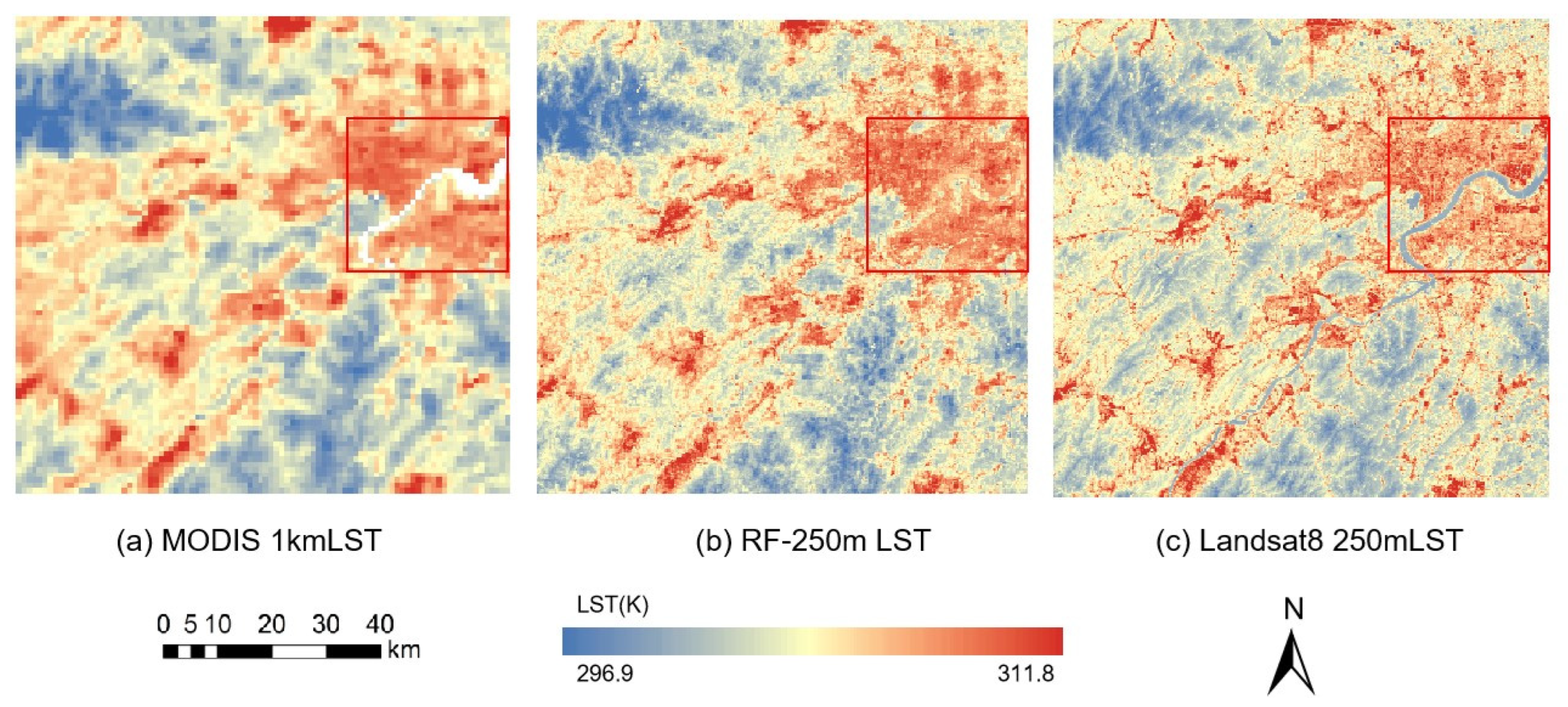
In Figure 4, it can be observed that the MODIS-retrieved LST exhibits gaps in water surface areas (indicated by the red box). In this study, the constructed RF-WST model was utilized to fit the surface temperature for the water body regions. The fitting results are presented in Figure 5.

In is evident in Figure 5a that there is a notable issue where the water surface temperatures cannot be distinctly differentiated from the surface temperatures of the surrounding land areas. This lack of clear distinction complicates the accurate representation of thermal dynamics in water bodies.

In contrast, after applying the RF-WST model to the 250 m LST results in Figure 5b, a more pronounced separation between the water surface temperatures and the underlying LST can be observed. The optimization provided by the RF-WST model effectively enhances the accuracy of the water temperature estimates, allowing for a clearer understanding of the spatial variations in temperature around aquatic environments.

In

Table 4. Comparison of LST accuracy before and after applying the RF-WST model.

	R	RMSE (K)
RF-250 m	0.8153	3.2882
RF-WST	0.8214	3.2714

, it can be observed that after applying the RF-WST model, the R value for the LST prediction results improved by 0.0061, while the RMSE decreased by 0.0168 K. This indicates that the RF-WST model effectively optimized the downscaled 250 m LST results to a certain extent, successfully addressing the issue of missing water body temperature retrievals in the MODIS data.

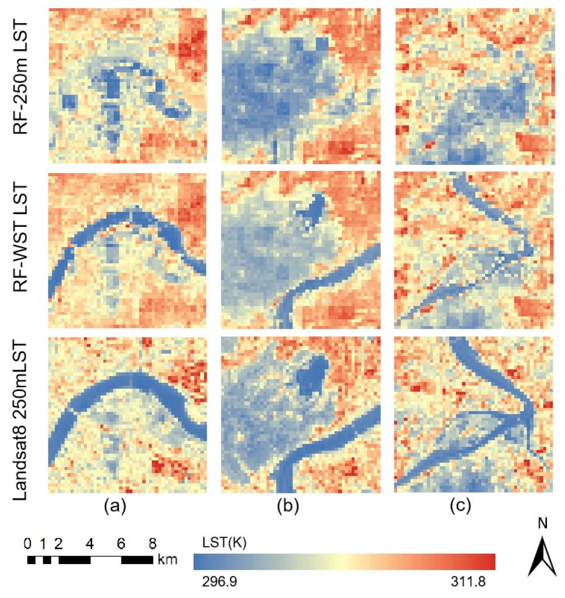
To further validate the enhancement in the water body regions, three different water body areas that previously showed voids in the MODIS LST data were selected for comparison.

In Figure 6, it is evident that after the optimization of water surface temperatures using the RF-WST model, the LST in water body areas contains more detailed information than the LST obtained from the RF-250 m model. Additionally, there is a clear distinction between the temperatures of the water bodies and the surrounding LST. This observation demonstrates that the RF-WST model exhibits good stability and reliability in accurately capturing water surface temperatures.

In

Table 5. Comparison of LST accuracy before and after applying the RF-WST model for different water bodies.

	a		b		c
	R	RMSE (K)	R	RMSE (K)	R	RMSE (K)
RF-250 m	0.4508	4.4004	0.7613	3.8869	0.5917	3.9207
RF-WST	0.7480	4.1943	0.8315	3.8300	0.6728	3.8528
Error	+0.2917	−0.2016	+0.0702	−0.0569	+0.0811	−0.0678

, the Landsat 8-retrieved LST serves as the true value to evaluate the R and the RMSE for the RF-250 m, RF-WST, and Landsat 8 results. The improvements in correlation coefficients for regions a, b, and c were 0.2971, 0.0702, and 0.0811, respectively, while the RMSE decreased by 0.2016 K, 0.0569 K, and 0.0678 K for the same regions.

Region a features a larger water surface area with a clear boundary from the surrounding land, resulting in the most pronounced improvement in fitting performance with the RF-WST model.

Region b, which encompasses both lakes and rivers, demonstrated that the RF-WST model effectively captured the surface temperatures of these water bodies, highlighting its reliability in various aquatic contexts.

Region c exhibited poorer model fitting performance, which was likely due to the narrow configuration of the water bodies combined with the 250 m spatial resolution of the imagery, which impacted the accuracy of the model simulations.

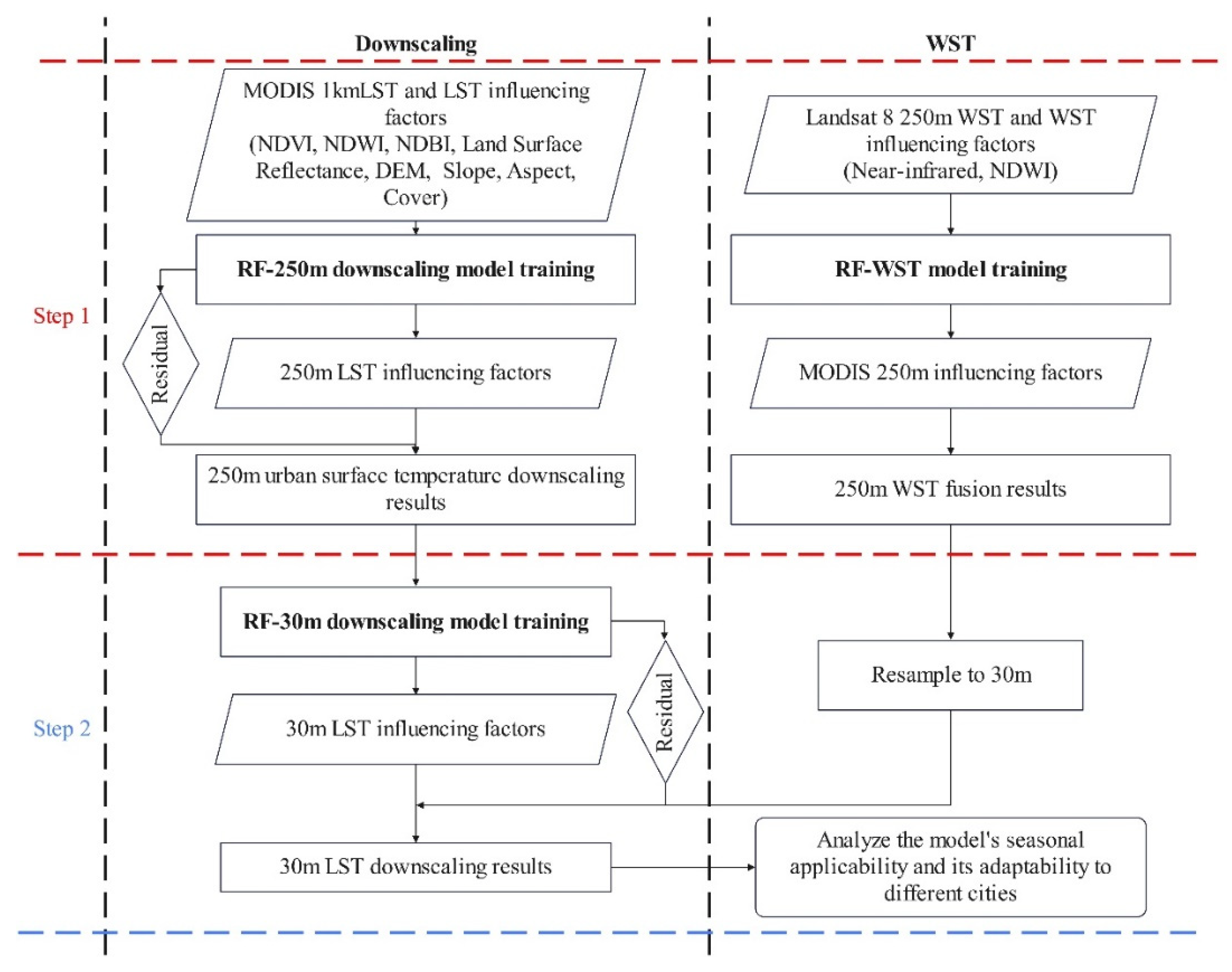
3.3. Results of 30 m Downscaling and Analysis

Based on the selected influencing factors—DEM, ASPECT, SLOPE, and COVER—the optimal model parameters were input to construct the second-step downscaling model, RF-30 m. The coarse-resolution LST data in the RF-30 m model were derived from the LST outputs of the RF-WST model. The RF-30 m model calculates the fitted LST values, which are then used to compute the residuals in comparison with the outputs from RF-WST. With the 30 m resolution influencing factors, fitted LST values at 30 m are obtained, and these are combined with the residuals, resulting in the final downscaled 30 m LST estimates.

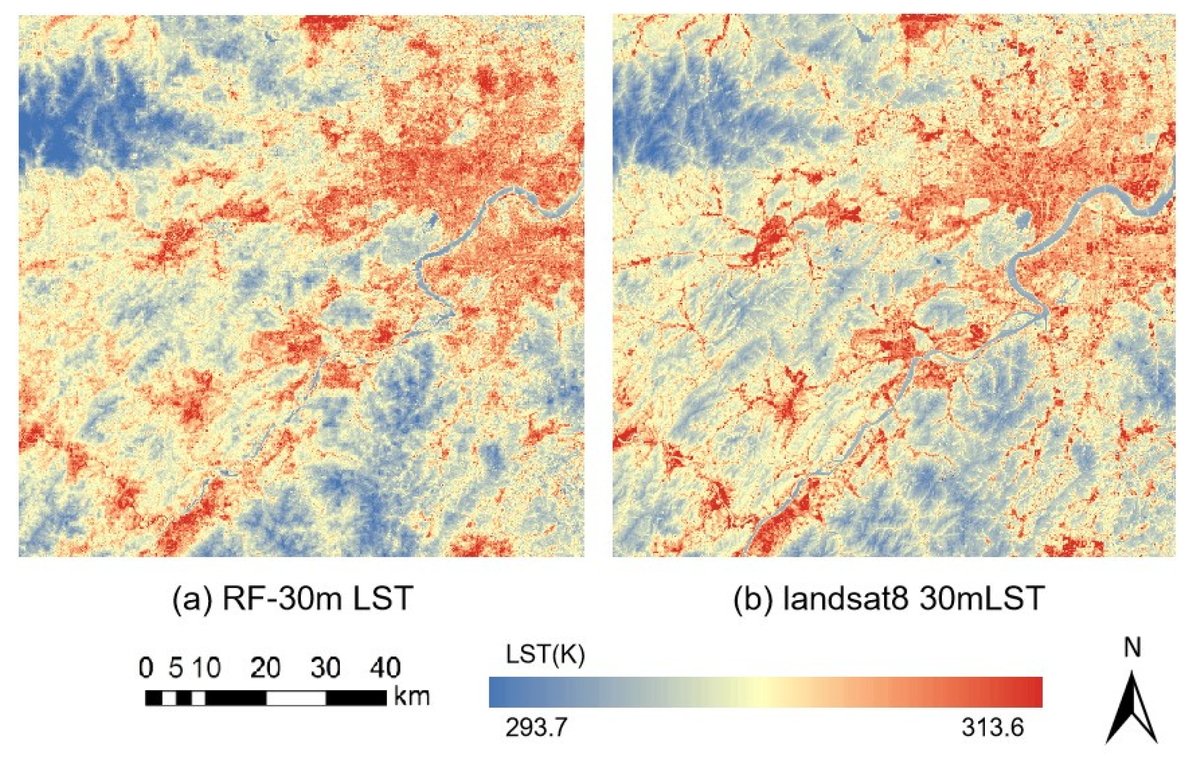
In Figure 7, it is evident that after the downscaling with the RF-30 m model, the overall spatial distribution of LST shows a high degree of consistency with that of Landsat 8. When compared with the 30 m LST from Landsat 8, the R value was found to be 0.8142, and the RMSE was 3.4172 K. These results fall within an acceptable error range, demonstrating that the RF-30 m model exhibits good accuracy.

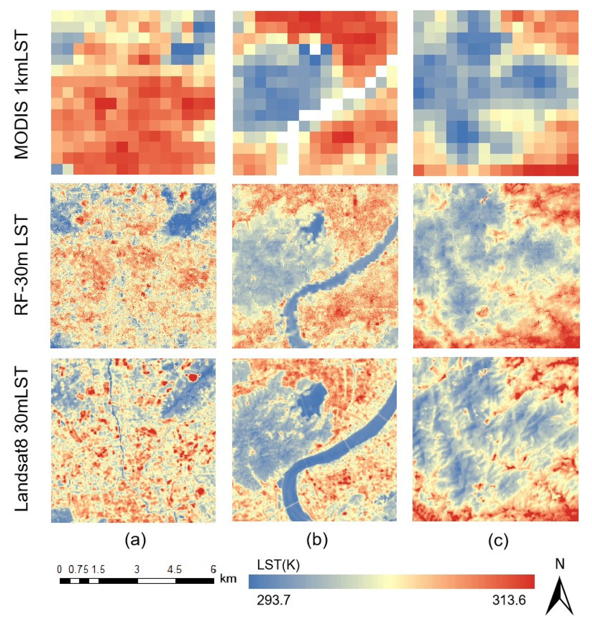
To further assess the effectiveness of the downscaling results, this study conducted comparisons across three distinct regions, urban, water, and vegetation, as depicted in Figure 8a–c.

Analysis of Figure 7 indicates that in the urban area (a), the RF-30 m model markedly enhances the detail of the LST; however, it does exhibit a tendency to overestimate surface temperatures within this region. In the water body area (b), the RF-30 m model effectively distinguishes the water surfaces from surrounding land areas, successfully addressing the voids in MODIS LST data. Nonetheless, some jagged artifacts are observable along the water boundaries. For the vegetation area (c), the overall distribution of surface temperatures is consistent with the validation data, yet the model does not adequately capture effects such as shading caused by mountainous terrain.

According to the data presented in

Table 6. Accuracy assessment of RF-30 m LST in different regions.

	Urban	Water	Vegetation
R	0.6795	0.7880	0.8606
RMSE (K)	4.7980	4.1951	1.5694

, the R value for the urban and water regions are 0.6795 and 0.7880, respectively, with corresponding RMSE values of 4.7980 K and 4.1951 K. In contrast, the vegetation region demonstrates a superior correlation coefficient of 0.8606 and a significantly lower RMSE of 1.5694 K, indicating that the downscaling performance is notably more effective in the vegetation area than in the urban and water regions.

3.4. Analysis of the Applicability of the Downscaling Model

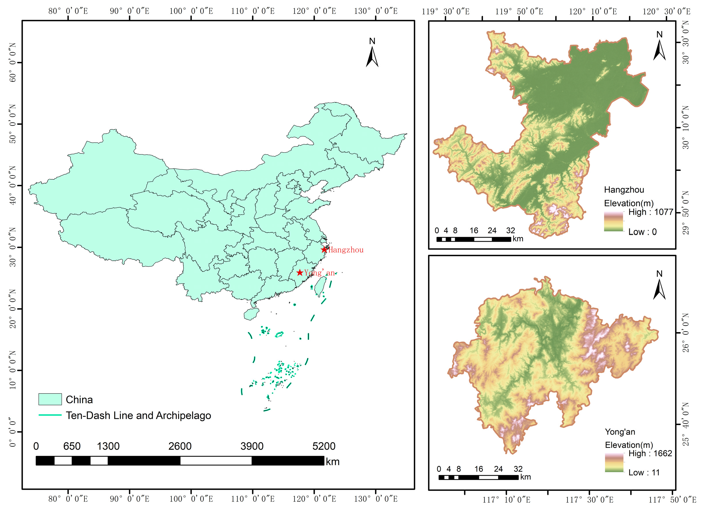
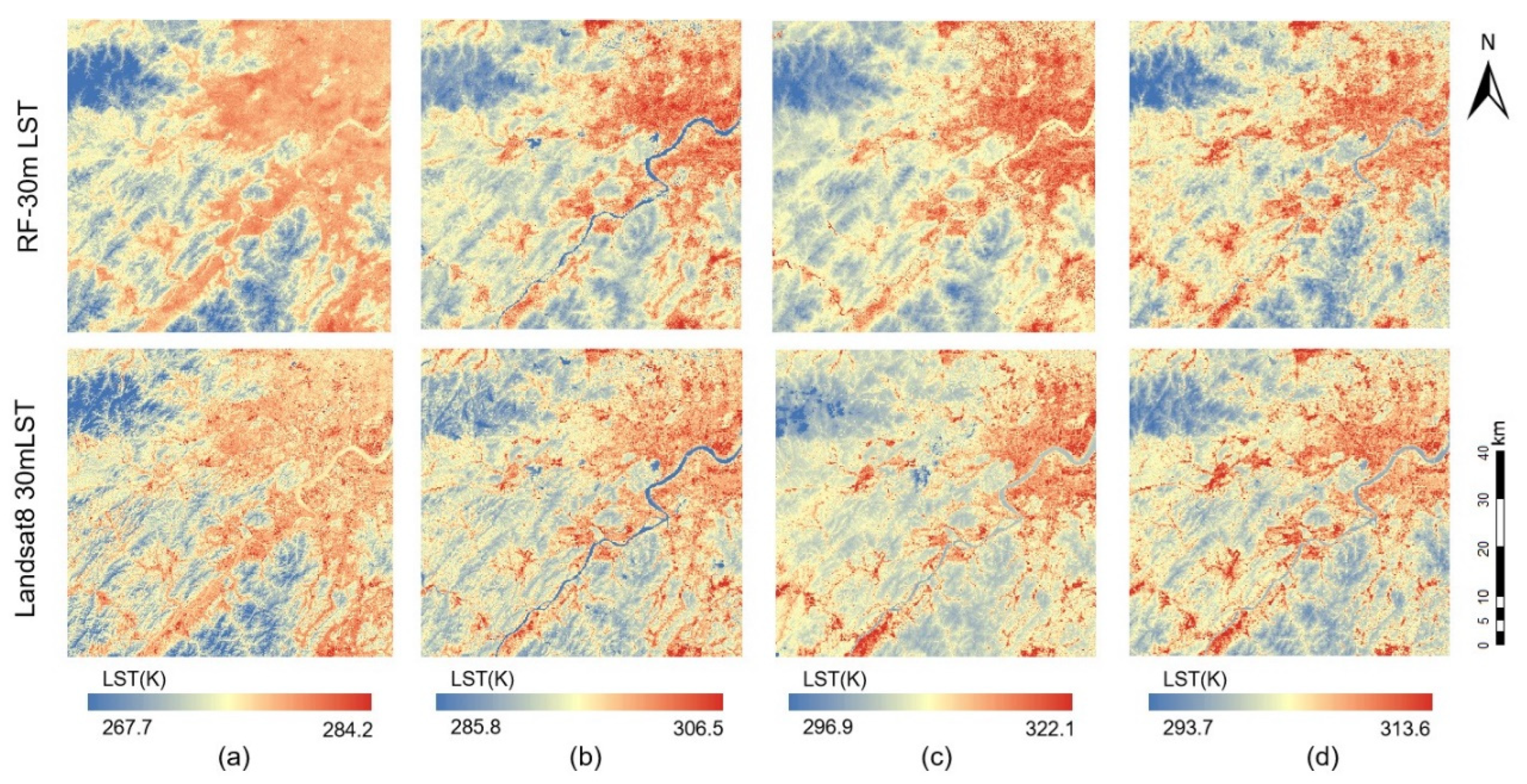
To further validate the applicability of the downscaling model across the four seasons, this study selected key dates, 28 January 2023, 2 April 2023, and 29 July 2023, representing winter, spring, and summer, respectively. These dates were analyzed alongside the data from 6 September 2022, to assess the model’s seasonal effectiveness in Hangzhou.

The validation data for January and April were obtained from Landsat 8 imagery captured on the same dates. However, due to data availability issues, the validation data for 29 July 2023, were sourced from the preceding day’s Landsat 8 imagery from 28 July 2023. Figure 9 presents a comparative analysis of the downscaling model’s application in Hangzhou across the four seasons.

Table 7. Accuracy verification of the RF-30 m LST in Hangzhou for different seasons.

	Winter	Spring	Summer	Autumn
R	0.8528	0.8185	0.7362	0.8142
RMSE (K)	1.6919	2.4759	6.2943	3.4172

provides the accuracy validation results for the different seasons. Overall, the downscaled LST exhibits a high degree of consistency in spatial distribution when compared with the Landsat LST data, meeting this study’s requirements.

In the seasonal analysis, it is observed that the model performs best in spring, where the spatial distribution of LST closely aligns with that of the Landsat data, as indicated by the high R and a low RMSE. In both autumn and winter, the model yields good downscaled results; however, there is a tendency to overestimate temperatures in urban areas. Conversely, in summer, the RMSE significantly increases, reflecting a poorer downscaling performance.

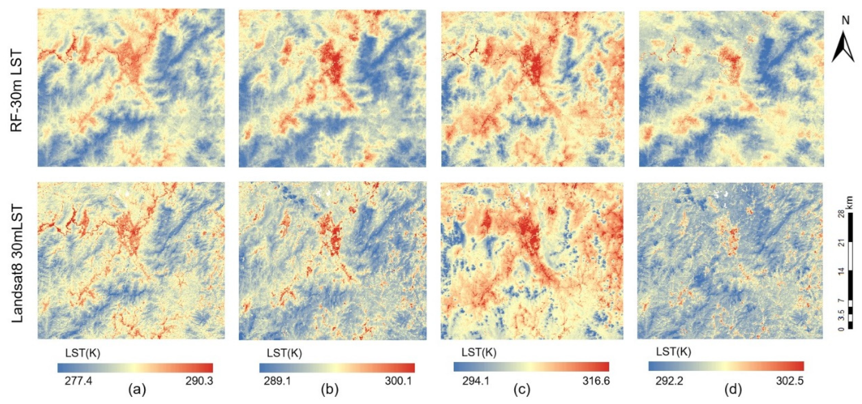
Considering the regional variability in the downscaling model’s performance, this study additionally selected seasonal data from Yong’an, Fujian Province, to compare the downscaling results. The seasonal data included the following dates: 18 December 2022, 9 April 2023, 11 July 2023, and 3 November 2023, representing winter, spring, summer, and autumn, respectively, for Yong’an. The 30-meter downscaling results for Yong’an across different seasons are presented in Figure 10.

In the figures, it is evident that the downscaled results for the winter and spring seasons show substantial agreement with the validation data in terms of the spatial distribution. However, during the summer, there is an observed overestimation of water body temperatures. In the autumn season, a general overestimation of temperatures in urban areas is noted, which aligns with the findings from the downscaled results for Hangzhou.

As indicated in

Table 8. Accuracy assessment of RF-30 m LST in Yong’an for different seasons.

	Winter	Spring	Summer	Autumn
R	0.8420	0.7626	0.7089	0.5575
RMSE (K)	1.4805	1.8227	7.7123	2.1740

, during the winter and spring seasons, the downscaled results exhibit high R and low RMSE values. Conversely, an increase in the RMSE is also observed during the summer months, which is similar to the trends noted previously. In the autumn season, the correlation coefficient is relatively low, indicating poorer model performance in capturing surface temperature dynamics during that period.

Considering the differences between the MODIS and Landsat sensors, discrepancies exist between the two LST results [26,27]. Therefore, the Landsat surface temperature data were resampled to a 1 km scale for comparison with the MODIS data. This allowed for an analysis of the systematic errors between the two datasets and an evaluation of the feasibility of the downscaled results.

Table 9. Comparative analysis of the MODIS 1 km LST and Landsat 1 km LST.

	Hang Zhou		Yong’an
	R	RMSE	R	RMSE
Winter	0.8155	1.6491	0.8068	1.5846
Spring	0.7601	2.3897	0.7189	1.8733
Summer	0.7496	6.0871	0.7302	7.6540
Autumn	0.7782	3.3116	0.5085	2.2152

presents the comparative results between Landsat 8 and MODIS data at 1 km spatial resolution for Hangzhou and Yong’an.

Based on an analysis of Table 7, Table 8 and Table 9, the following conclusions can be drawn:

(1) In Hangzhou, for the winter, spring, and autumn seasons, the downscaled RF-30 m LST shows an improvement in correlation (R) compared with the original MODIS data, with the RMSE values showing a modest increase, remaining below 0.2 K and, thus, within an acceptable error range. However, during the summer, the downscaled RF-30 m LST exhibits a reduction in R by 0.0134, while the RMSE increases by more than 0.2 K, which is inconsistent with the patterns observed in the other three seasons.

(2) In Yong’an, for the winter, spring, and autumn seasons, the downscaled RF-30 m LST shows an increase in correlation (R) compared with the original MODIS data, and the RMSE values decline. However, in the summer, the downscaled RF-30 m LST shows a decrease in R of 0.0213, along with an increase in RMSE of 0.0583 K.

(3) Combining the results from Hangzhou and Yong’an, it is evident that the downscaling model performs better in winter, spring, and autumn, while its performance is poorer in summer. The downscaled LST in the winter, spring, and autumn seasons shows improved correlation, with the RMSE also remaining within acceptable limits.

Based on the previous literature [28,29], it can be inferred that during the summer, the Landsat 8 imaging time used for validation is approximately half an hour later than that of MODIS. Given the higher temperatures in summer and the rapid warming of surface temperatures, the final LST data obtained from Landsat 8 are likely to be higher than the MODIS LST products. This discrepancy could contribute to the larger RMSE between the two datasets.

Moreover, in the downscaled RF-30 m LST results for the summer, some water body areas exhibit an overestimation of LST. This may be attributed to the fact that the RF-WST model was constructed using Landsat 8 LST data as the training dataset, which could lead to biased fitting results, resulting in the overestimation of water surface temperatures.

To better analyze the high-error phenomenon in the summer downscaling results, this study additionally selected data from Wuhan on 21 July 2024, and Beijing on 19 July 2023, for downscaling. These results were then compared with the summer downscaling results of Hangzhou and Yong’an from this study.

Table 10. Comparison of summer downscaling results across different cities.

	Hangzhou	Yong’an	Wuhan	Beijing
R	0.7362	0.7089	0.7288	0.6049
RMSE (K)	6.2943	7.7123	8.4767	8.3668

presents the validation results by comparing the summer downscaling outcomes of the four cities with the Landsat 8 data.

As shown in the table, the downscaling results for multiple summer time series across the four cities exhibit relatively high RMSE values when compared with the Landsat 8 data. This indicates certain limitations in the model’s performance during the summer downscaling process. Notably, Beijing and Wuhan have more complex underlying surface distributions and a wider spread of impervious surfaces compared with the other cities, which impacts the model’s fitting accuracy.

4. Discussion

Considering the spatiotemporal resolution limitations of satellite sensors, land surface temperature (LST) downscaling plays a crucial role in the study of continuous thermal environments. Over the past two decades, numerous models [30,31] have been proposed for LST downscaling. However, these models often rely on parameters derived from different satellite sensors [32,33,34], resulting in low continuity in the actual downscaled results. Water surface temperature is an essential component of LST. However, in MODIS LST products, large water bodies (exceeding 1 km in size) frequently appear as null values due to spatial resolution constraints [35,36]. To address this issue, this study introduces a novel downscaling method that not only enhances LST accuracy but also compensates for missing water surface temperatures, thereby complementing existing models.

Most existing LST downscaling approaches employ linear regression to establish relationships between LST and its influencing factors [37]. However, these relationships are often nonlinear, making simple linear regression inadequate. In this study, an RF model is utilized to capture the complex nonlinear interactions between the LST and its influencing factors, significantly improving downscaling accuracy. In terms of variable selection, previous studies often used high-resolution remote sensing data from various satellite sensors, leading to inconsistencies between these high-resolution datasets and the coarse-resolution LST data that they aimed to refine [38,39]. To minimize these discrepancies, this study carefully selects downscaling predictors exclusively from MODIS-derived remote sensing data, ensuring a unified data source and reducing the impact of multisensor inconsistencies on downscaling results. Since MODIS LST data have a daily temporal resolution, the downscaled results in this study maintain the same temporal resolution, ensuring the continuity of temperature variation over time. This provides a more reliable reference for analyzing continuous LST changes and offers robust data support for thermal environment studies. Furthermore, to ensure the applicability of the proposed downscaling model, its performance was evaluated across different cities and seasons. The results demonstrate that the model exhibits strong adaptability, making it broadly applicable across cities with diverse climatic backgrounds. This improved downscaling approach provides more precise temperature datasets, offering valuable insights for urban planning and sustainable development.

This research employs three models: RF-250 m, RF-WST, and RF-30 m. In the RF-250 m model, LST is downscaled from 1 km to 250 m using selected LST-influencing factors. In contrast to previous studies, this work exclusively utilizes MODIS-derived remote sensing data, minimizing errors associated with integrating data from multiple satellite sensors and, thus, enhancing the model’s feasibility.

Although previous research has focused little on downscaling water body areas [40], WST plays a critical role in LST. After downscaling, WST often homogenizes with the surrounding land temperature due to the increased spatial resolution. To mitigate this issue, the RF-WST model was introduced to effectively distinguish water bodies from surrounding land surfaces and preserve the temperature contrast.

The RF-30 m model further improves spatial detail in the downscaled LST, providing more refined information than that of the original MODIS data. However, the model exhibits larger errors during the summer months, which can be attributed to the half-hour temporal discrepancy between the MODIS and Landsat 8 acquisitions. This time gap leads to discrepancies in surface temperatures, particularly in high-temperature urban areas. This study conducted a comparative analysis of summer downscaling results across different cities, revealing that the downscaled outputs for all four cities exhibit a high degree of similarity. The RMSE in each case exceeds 6 K, indicating that the model encounters common challenges when applied to urban areas during the summer. Urban environments feature complex underlying surface distributions, where the presence of impervious surfaces plays a critical role in shaping the LST. In these areas, summer LST is particularly sensitive to air temperature variations, and its response is further influenced by the physical properties of impervious surfaces [41]. Factors such as material composition and surface color significantly impact heat absorption and retention—for instance, darker surfaces and heat-absorbing materials contribute to elevated LSTs. Additionally, the widespread use of cooling systems in urban areas further affects the thermal environment. Increased energy consumption and anthropogenic heat emissions exacerbate the urban heat island effect, intensifying localized temperature variations [42]. The downscaling model used in this study incorporates impervious surface parameters such as the NDBI and land-cover-type data. However, it lacks key socioeconomic and urban morphology factors, such as population density and building height, which are crucial in accurately capturing LST variations in urban environments. As a result, the model exhibits certain limitations in fitting impervious surface areas, highlighting the need for more comprehensive datasets to enhance downscaling accuracy in complex urban landscapes.

The model was applied to Hangzhou and Yong’an, demonstrating its feasibility to some extent. However, this study’s limited consideration of different urban climates indicates that further testing across diverse environments is needed. We acknowledge that integrating climatic predictors could improve the model’s seasonal robustness, and we plan to explore this in future work. Moreover, the research relied solely on Landsat 8 data, which, while spatially consistent with MODIS, introduces temporal mismatches. Future validation efforts should incorporate more ground-based data to further enhance model accuracy.

In conclusion, this study successfully downscaled MODIS LST data from the MOD11A1 product using the RF-250 m, RF-WST, and RF-30 m models, resulting in LST products with 30 m spatial resolution and a 1-day temporal resolution. The introduction of the WST model effectively compensates for missing water temperature data in MODIS, offering a valuable tool for urban LST research and the study of urban heat islands. This study demonstrates high downscaling accuracy in vegetation and water body regions, providing reliable data support for evidence-based policy development. Given the significant role of vegetation and water bodies in regulating urban temperatures, policymakers could consider expanding their distribution in areas with intense urban heat island effects. This strategic approach could help mitigate heat stress, creating a more comfortable and sustainable living environment for urban populations.

5. Conclusions

This study successfully employed a TSDM approach to generate high-spatial-resolution (30 m) and high-temporal-resolution (1 day) LST data by integrating MODIS remote sensing data with machine learning models. The key findings are as follows:

The RF-250 m and RF-30 m models demonstrated strong downscaling performance, achieving higher resolution while preserving consistent spatial distributions of LST. Seasonal analysis revealed that the models performed optimally in winter, spring, and autumn, with reduced accuracy in summer due to environmental and temporal factors.

The proposed RF-WST model effectively addressed gaps in water surface temperature data, significantly improving LST estimation in water body regions. However, the model faced challenges under summer conditions, which were attributed to rapid temperature fluctuations and limitations in its parameterization.

The models exhibited better downscaling performance in Yong’an than in Hangzhou, highlighting their adaptability to different regions and environmental conditions.

Overall, this study demonstrates the feasibility of using a machine learning-based TSDM approach to produce high-resolution LST data, providing valuable insights for monitoring and analyzing thermal environments across diverse landscapes.

References

1. Li, Z.; Tang, B.; Wu, H.; Ren, H.; Yan, G.; Wan, Z.; Trigo, I.F.; Sobrino, J.A. Satellite-derived land surface temperature: Current status and perspectives. Remote Sens. Environ. 2013, 131, 14–37. [Google Scholar] [CrossRef]
2. Shui, C.; Shan, B.; Li, W.; Wang, L.; Liu, Y. Investigating the influence of land cover on land surface temperature. Adv. Space Res. 2024, 75, 2614–2631. [Google Scholar] [CrossRef]
3. Anderson, M.C.; Allen, R.G.; Morse, A.; Kustas, W.P. Use of Landsat thermal imagery in monitoring evapotranspiration and managing water resources. Remote Sens. Environ. 2012, 122, 50–65. [Google Scholar] [CrossRef]
4. Kustas, W.P.; Norman, J.M.; Anderson, M.C.; French, A.N. Estimating subpixel surface temperatures and energy fluxes from the vegetation index–radiometric temperature relationship. Remote Sens. Environ. 2003, 85, 429–440. [Google Scholar] [CrossRef]
5. Agam, N.; Kustas, W.P.; Anderson, M.C.; Li, F.; Neale, C.M.U. A vegetation index based technique for spatial sharpening of thermal imagery. Remote Sens. Environ. 2007, 107, 545–558. [Google Scholar] [CrossRef]
6. Gao, F.; Masek, J.; Schwaller, M.; Hall, F. On the blending of the Landsat and MODIS surface reflectance: Predicting daily Landsat surface reflectance. IEEE Trans. Geosci. Remote Sens. 2006, 44, 2207–2218. [Google Scholar] [CrossRef]
7. Wu, P.; Shen, H.; Ai, T.; Liu, Y. Land-surface temperature retrieval at high spatial and temporal resolutions based on multi-sensor fusion. Int. J. Digit. Earth 2013, 6, 113–133. [Google Scholar] [CrossRef]
8. Hutengs, C.; Vohland, M. Downscaling land surface temperatures at regional scales with random forest regression. Remote Sens. Environ. 2016, 178, 127–141. [Google Scholar] [CrossRef]
9. Li, W.; Ni, L.; Li, Z.L.; Duan, S.B.; Wu, H. Evaluation of Machine Learning Algorithms in Spatial Downscaling of MODIS Land Surface Temperature. IEEE J. Sel. Top. Appl. Earth Observ. Remote Sens. 2019, 12, 2299–2307. [Google Scholar] [CrossRef]
10. Wu, H.; Li, W. Downscaling Land Surface Temperatures Using a Random Forest Regression Model with Multitype Predictor Variables. IEEE Access 2019, 7, 21904–21916. [Google Scholar] [CrossRef]
11. Ouyang, X.; Dou, Y.; Yang, J.; Chen, X.; Wen, J. High Spatiotemporal Rugged Land Surface Temperature Downscaling over Saihanba Forest Park, China. Remote Sens. 2022, 14, 2617. [Google Scholar] [CrossRef]
12. Xu, S.; Zhao, Q.; Yin, K.; He, G.; Zhang, Z.; Wang, G.; Wen, M.; Zhang, N. Spatial Downscaling of Land Surface Temperature Based on a Multi-Factor Geographically Weighted Machine Learning Model. Remote Sens. 2021, 13, 1186. [Google Scholar] [CrossRef]
13. Wu, P.; Yin, Z.; Zeng, C.; Duan, S.B.; Göttsche, F.M.; Ma, X.; Li, X.; Yang, H.; Shen, H. Spatially Continuous and High-Resolution Land Surface Temperature Product Generation: A Review of Reconstruction and Spatiotemporal Fusion Techniques. IEEE Geosci. Remote Sens. Mag. 2021, 9, 112–137. [Google Scholar] [CrossRef]
14. Ezimand, K.; Chahardoli, M.; Azadbakht, M.; Matkan, A.A. Spatiotemporal analysis of land surface temperature using multi-temporal and multi-sensor image fusion techniques. Sustain. Cities Soc. 2021, 64, 102508. [Google Scholar] [CrossRef]
15. Wang, R.; Gao, W.; Peng, W. Downscale MODIS Land Surface Temperature Based on Three Different Models to Analyze Surface Urban Heat Island: A Case Study of Hangzhou. Remote Sens. 2020, 12, 2134. [Google Scholar] [CrossRef]
16. Peng, Y.; Li, W.; Luo, X.; Li, H. A Geographically and Temporally Weighted Regression Model for Spatial Downscaling of MODIS Land Surface Temperatures Over Urban Heterogeneous Regions. IEEE Trans. Geosci. Remote Sens. 2019, 57, 5012–5027. [Google Scholar] [CrossRef]
17. Firozjaei, M.K.; Mijani, N.; Kiavarz, M.; Duan, S.; Atkinson, P.M.; Alavipanah, S.K. A novel surface energy balance-based approach to land surface temperature downscaling. Remote Sens. Environ. 2024, 305, 114087. [Google Scholar] [CrossRef]
18. Guo, F.; Hu, D.; Schlink, U. A new nonlinear method for downscaling land surface temperature by integrating guided and Gaussian filtering. Remote Sens. Environ. 2022, 271, 112915. [Google Scholar] [CrossRef]
19. Dong, P.; Zhan, W.; Wang, C.; Jiang, S.; Du, H.; Liu, Z.; Chen, Y.; Li, L.; Wang, S.; Ji, Y. Simple yet efficient downscaling of land surface temperatures by suitably integrating kernel- and fusion-based methods. ISPRS-J. Photogramm. Remote Sens. 2023, 205, 317–333. [Google Scholar] [CrossRef]
20. Wu, J.; Xia, L.; On Chan, T.; Awange, J.; Zhong, B. Downscaling land surface temperature: A framework based on geographically and temporally neural network weighted autoregressive model with spatio-temporal fused scaling factors. ISPRS-J. Photogramm. Remote Sens. 2022, 187, 259–272. [Google Scholar] [CrossRef]
21. Dong, P.; Gao, L.; Zhan, W.; Liu, Z.; Li, J.; Lai, J.; Li, H.; Huang, F.; Tamang, S.K.; Zhao, L. Global comparison of diverse scaling factors and regression models for downscaling Landsat-8 thermal data. ISPRS-J. Photogramm. Remote Sens. 2020, 169, 44–56. [Google Scholar] [CrossRef]
22. Jaafar, H.; Mourad, R.; Schull, M. A global 30-m ET model (HSEB) using harmonized Landsat and Sentinel-2, MODIS and VIIRS: Comparison to ECOSTRESS ET and LST. Remote Sens. Environ. 2022, 274, 112995. [Google Scholar] [CrossRef]
23. Burnett, M.; Chen, D. The Impact of Seasonality and Land Cover on the Consistency of Relationship between Air Temperature and LST Derived from Landsat 7 and MODIS at a Local Scale: A Case Study in Southern Ontario. Land 2021, 10, 672. [Google Scholar] [CrossRef]
24. Laraby, K.G.; Schott, J.R. Uncertainty estimation method and Landsat 7 global validation for the Landsat surface temperature product. Remote Sens. Environ. 2018, 216, 472–481. [Google Scholar] [CrossRef]
25. Negahbani, S.; Momeni, M.; Moradizadeh, M. Improving the Spatiotemporal Resolution of Soil Moisture Through a Synergistic Combination of MODIS and LANDSAT8 Data. Water Resour. Manag. 2022, 36, 1813–1832. [Google Scholar] [CrossRef]
26. Zhou, F.; Zhong, D. Kalman filter method for generating time-series synthetic Landsat images and their uncertainty from Landsat and MODIS observations. Remote Sens. Environ. 2020, 239, 111628. [Google Scholar] [CrossRef]
27. Che, X.; Zhang, H.K.; Liu, J. Making Landsat 5, 7 and 8 reflectance consistent using MODIS nadir-BRDF adjusted reflectance as reference. Remote Sens. Environ. 2021, 262, 112517. [Google Scholar] [CrossRef]
28. Lu, M.; Chen, J.; Tang, H.; Rao, Y.; Yang, P.; Wu, W. Land cover change detection by integrating object-based data blending model of Landsat and MODIS. Remote Sens. Environ. 2016, 184, 374–386. [Google Scholar] [CrossRef]
29. Williamson, S.N.; Hik, D.S.; Gamon, J.A.; Jarosch, A.H.; Anslow, F.S.; Clarke, G.K.C.; Scott Rupp, T. Spring and summer monthly MODIS LST is inherently biased compared to air temperature in snow covered sub-Arctic mountains. Remote Sens. Environ. 2017, 189, 14–24. [Google Scholar] [CrossRef]
30. Xu, F.; Zhu, X.; Chen, J.; Zhan, W. A stepwise unmixing model to address the scale gap issue present in downscaling of geostationary meteorological satellite surface temperature images. Remote Sens. Environ. 2024, 306, 114141. [Google Scholar] [CrossRef]
31. Adeyeri, O.E.; Folorunsho, A.H.; Ayegbusi, K.I.; Bobde, V.; Adeliyi, T.E.; Ndehedehe, C.E.; Akinsanola, A.A. Land surface dynamics and meteorological forcings modulate land surface temperature characteristics. Sustain. Cities Soc. 2024, 101, 105072. [Google Scholar] [CrossRef]
32. Pu, R. Assessing scaling effect in downscaling land surface temperature in a heterogenous urban environment. Int. J. Appl. Earth Obs. Geoinf. 2021, 96, 102256. [Google Scholar] [CrossRef]
33. Sattari, F.; Hashim, M.; Sookhak, M.; Banihashemi, S.; Pour, A.B. Assessment of the TsHARP method for spatial downscaling of land surface temperature over urban regions. Urban Clim. 2022, 45, 101265. [Google Scholar] [CrossRef]
34. Güngör Şahin, O.; Gündüz, O. A novel land surface temperature reconstruction method and its application for downscaling surface soil moisture with machine learning. J. Hydrol. 2024, 634, 131051. [Google Scholar] [CrossRef]
35. Aguilar-Lome, J.; Soca-Flores, R.; Gómez, D. Evaluation of the Lake Titicaca’s surface water temperature using LST MODIS time series (2000–2020). J. S. Am. Earth Sci. 2021, 112, 103609. [Google Scholar] [CrossRef]
36. Lazhu; Yang, K.; Qin, J.; Hou, J.; Lei, Y.; Wang, J.; Huang, A.; Chen, Y.; Ding, B.; Li, X. A Strict Validation of MODIS Lake Surface Water Temperature on the Tibetan Plateau. Remote Sens. 2022, 14, 5454. [Google Scholar] [CrossRef]
37. Yoo, C.; Im, J.; Park, S.; Cho, D. Spatial downscaling of MODIS land surface temperature: Recent research trends, challenges, and future directions. Korean J. Remote Sens. 2020, 36, 609–626. [Google Scholar]
38. Mao, Q.; Peng, J.; Wang, Y. Resolution enhancement of remotely sensed land surface temperature: Current status and perspectives. Remote Sens. 2021, 13, 1306. [Google Scholar] [CrossRef]
39. Zhu, X.; Song, X.; Leng, P.; Li, X.; Gao, L.; Guo, D.; Cai, S. A framework for generating high spatiotemporal resolution land surface temperature in heterogeneous areas. Remote Sens. 2021, 13, 3885. [Google Scholar] [CrossRef]
40. Jia, T.; Yang, K.; Peng, Z.Q.; Tang, L.; Duan, H.; Luo, Y. Review on the change trend, attribution analysis, retrieval, simulation, and prediction of lake surface water temperature. IEEE J. Sel. Top. Appl. Earth Obs. Remote Sens. 2022, 15, 6324–6355. [Google Scholar] [CrossRef]
41. Morabito, M.; Crisci, A.; Georgiadis, T.; Orlandini, S.; Munafò, M.; Congedo, L.; Rota, P.; Zazzi, M. Urban imperviousness effects on summer surface temperatures nearby residential buildings in different urban zones of Parma. Remote Sens. 2018, 10, 26. [Google Scholar] [CrossRef]
42. He, Y.; Pu, N.; Zhang, X.; Wu, C.; Tang, W. Long-Term Spatiotemporal Heterogeneity and Influencing Factors of Remotely Sensed Regional Heat Island Effect in the Central Yunnan Urban Agglomeration. Land 2025, 14, 232. [Google Scholar] [CrossRef]
Figure 1. Study area.
Atmosphere 16 00424 g001
Figure 2. Parameter learning curves.
Atmosphere 16 00424 g002
Figure 3. Experimental flowchart.
Atmosphere 16 00424 g003
Figure 4. Spatial distribution of LST in the main urban area of Hangzhou.
Atmosphere 16 00424 g004
Figure 5. Comparison of the RF-WST model before and after. (a) displays the LST obtained after applying the RF-250 m model for downscaling. (b) shows the optimized 250 m LST after applying the RF-WST model.
Atmosphere 16 00424 g005
Figure 6. LST comparison chart for water regions. (a) Water body area 1 (b) Water body area 2 (c) Water body area 3.
Atmosphere 16 00424 g006
Figure 7. LST comparison chart of the RF-30 m model.
Atmosphere 16 00424 g007
Figure 8. Comparison chart of 30 m RF downscaling TEM results. (a) urban, (b) water, and (c) vegetation.
Atmosphere 16 00424 g008
Figure 9. Seasonal LST downscaling results for Hangzhou. (a) shows the downscaled LST results for Hangzhou on 28 January 2023, representing winter; (b) displays the downscaled LST results for 2 April 2023, representing spring; (c) illustrates the downscaled LST results for 29 July 2023, representing summer; and (d) presents the downscaled LST results for 6 September 2022, representing autumn.
Atmosphere 16 00424 g009
Figure 10. Seasonal LST downscaling map of Yong’an. (a) displays the downscaled LST results for Yong’an City on 18 December 2022; (b) shows the downscaled LST results for Yong’an on 9 April 2023; (c) presents the downscaled LST results for Yong’an on 11 July 2023; and (d) depicts the downscaled LST results for Hangzhou on 3 November 2023.
Atmosphere 16 00424 g010