Urban Microclimates in Action! High-Resolution Temperature and Humidity Differences Across Diverse Urban Terrain ^†

Abstract

With more than half of the world already living in urban spaces—a number set to increase in the coming decades—the need is clear to understand urban microclimates and extremes. This study placed twenty MX2302a HOBOmobile weather microsensors placed in aerated housings across the ~4 km² of the campus of the University of South Alabama from September to November 2022 and recorded temperature, relative humidity, and dewpoint every minute during the study period. These sensors were placed in situ, which allowed for the diversity in land cover, canopy cover, and aspect—large microclimatic drivers—to be captured. Sensors were compared to a campus mesonet station, part of the South Alabama Mesonet, a member of the National Mesonet Program. During the study period, temperatures were found to vary as much as 13 °C at the same minute across campus, with substantial changes in humidities and dewpoints also found. For example, the campus mesonet may have read 32 °C, yet the sensors could read as low as 29 °C and as high as 42 °C at the same moment. This study shows that the world is far more complex than what is seen at the mesoscale under idealized conditions, and the implications for society are considered.

1. Introduction

The meteorological world is one that is built on a foundation of networks of mesoscale and synoptic scale weather stations. In the United States, one can obtain data from ASOS stations, an assortment of state or regional level mesonets, remote measures, computer models, COOP networks, ocean buoys, weather balloons, and other sources often at a one-minute timescale. These observed data are then used for forecasts and decision making and disseminated to the general public for use. When a person checks their chosen weather application on their phone or accesses their preferred website, they are being given information that originated in some way from this network [1]. Yet, mesoscale weather processes—and the networks of stations that record them—do not always resolve processes that occur on a microscale [2,3,4]. Processes and phenomena operating on a microscale can be entirely missed as a result, meaning mesoscale networks only show part of a larger, far more complex, picture at the microscale [5,6,7].

It is estimated that approximately 56% of the nearly eight billion people who inhabit this planet currently live in cities. This has been following a trend—one of increased urbanization—that has been ongoing for the last several centuries, and it is expected that by the year 2050, approximately 70% of the global population will live in urban spaces [8]. This makes the study of urban and suburban microclimates imperative. The urban heat island comes from the altering of surface energy budgets stemming from high surface variability in urban spaces. These changes to surface energy budgets can lead to large differences in microclimate responses to what is, effectively, the same meso-scale meteorological conditions [9,10,11]. This is particularly the case when regarding extremes (temperature, rainfall, heat indices, etc.). Placing more people within urban spaces in the coming decades is expected to exacerbate this concern [12,13,14]. As such, studies of microclimates and micrometeorologies within urban spaces are more important than ever.

Microclimates, generally speaking, are created and driven by the land cover, canopy cover, and topographic exposure [15,16,17] of a particular point and can exist with extensive diversity across even a small space depending on the spatiotemporal resolution of those studying them [18,19,20]. Surface energy budgets vary based on insolation and its interactions with the surface and in an area of heterogeneous land covers, and these budgets can vary immensely over relatively small spaces [21].

One field that applies this idea is the urban heat island (UHI); with studies dating back to the 1800s, the phenomenon has been well-studied ever since [22,23,24]. However, there are numerous methods to study this phenomenon. In the present, numerous studies have focused on either remotely sensed studies at specific scales, the use of mobile or fixed ground observation networks, drone technology, or computer-simulated models based on observed data [25,26,27,28,29]. While these studies have advanced the field immensely, they are typically limited by either spatial or temporal resolution or are limited by the length of study. However, the placement of weather sensors within urban spaces is a method that is being used more often. Beginning with the Balchin and Pye studies of the English town of Bath in the late 1940s [30,31,32], the idea of placing weather stations in and around an urbanized space has shown that temperatures, humidities, and precipitation amounts can vary immensely over even small spaces. While the idea of directly studying urban microclimates with in situ sensors operating at a one-minute timescale was not feasible decades ago, this is now possible due to improvements in technology and cost [33,34]. The recent studies have shown that complex urban terrain can lead to immense changes in conditions over small spaces and that during sunny, daytime conditions, one can expect large temperature differences at the same moment over even a few square miles [35,36]. Reasons for this can mostly be explained by the canopy layer—urban heat island (CL-UHI) effect, wherein urban areas are warmer in dry, fair-weather daytime conditions due to land cover, surface geometry, and the permeability of surfaces, being on full display [37].

While placing sensors in situ may not be up to the standards of a mesoscale network of weather stations, the goal is not to supersede such networks. This undergraduate student-driven study was performed to show the potential range in temperatures and humidities that could occur in highly diverse urban terrain and compare them to a mesonet station situated within the study area. Twenty weather sensors were placed across the University of South Alabama’s campus in Mobile, Alabama, and they recorded temperature, relative humidity, and dewpoint every minute during the months of September, October, and November 2022. Added to this dataset was the campus mesonet station, part of the University of South Alabama’s Mesonet, and comparisons of temperature, humidity, and heat index were made across all stations during the study period. The goal of this paper was to explore the range of temperatures and humidities experienced in a relatively small, yet highly diverse, land cover area. Observing and analyzing meteorological variables had not yet been carried out at such a high spatiotemporal scale (one-minute temporal scale, 21 sensors in a ~4 km² area). In particular, extreme events (heat, cold, heat index) were the primary focus of the study.

This article is an extended version of a paper entitled “Urban microclimates in action! High resolution temperature and humidity differences across diverse urban terrain”, which was presented at both the AGU Annual Meeting in December 2022 in Chicago [38] and 2024 AAG Annual Meeting in Honolulu [39]. However, this paper expanded the analysis and extended the discussion section significantly.

2. Materials and Methods

2.1. Study Area and Time

The University of South Alabama is located in Mobile, Alabama on a campus located in the western suburbs of the city. Mobile classifies as a Cfa Köppen Climate with hot summers and mild winters [40,41]. The study was performed in the late summer and fall months of 2022, a period characterized by significant temperature fluctuations, with both warmer and cooler-than-average conditions, though on average, it was slightly warmer than the climatological average. Rainfall was below average during the September to November 2022 time span, with nearly all of the Mobile, AL region falling under a D0 (abnormally dry) to D2 (severe drought) drought monitor status [42,43].

The campus is approximately 4 square kilometers in area and has a mix of land cover types ranging from heavily urbanized spaces to natural open water, forested, and wetland areas (Figure 1). Using the 2019 National Land Cover Dataset [44], the authors classified the campus into three types of land use: urban (44%), landscaped (28%), and natural (28%). Of the twenty stations, six were placed in urban spaces (near buildings, parking lots, streets), seven landscaped spaces (spaces which were grassy or surrounded by trees, but maintained by university grounds crews), and seven in natural areas (nature trails, river floodplain, unmanaged by grounds crews). As per the Local Climate Zones classifications from Stewart and Oke 2012 [45], the urban spaces were all “Open midrise” and “Open low-rise”, and the landscaped spaces were all “Sparsely built” or “Low plants”. The natural areas were either “Dense Trees” or “Scattered Trees”. These sites were chosen based on the availability of the site as per University regulations, potential diversity of land use types, aspect, and canopy cover with the goal to obtain a diverse set of potential microclimates that one could find across campus. The USA Mesonet station was located in an area classified as landscaped with a very light northeast-facing slope.

2.2. Equipment and Installation

Twenty MX2302a HOBOMobile Bluetooth-enabled sensors were placed in La Crosse Technology plastic aerated housings at each site. The aerated housings allow air to pass through while keeping the sensor protected from the elements. The housings were attached between 1.5 and 2 m off the ground, preferably on the west face of a tree, bush, stop sign, traffic post, or in one case, a quasi-structurally-sound footbridge via adjustable hose clamps on 16 September 2022. Data were recovered from each sensor by undergraduate students every two weeks, and the sensors would be checked during these visits, though no field adjustments or fixes were required during the study period. In order to confirm the accuracy and uniformity of the sensors, before being deployed, the sensors were placed in a controlled environment for 48 h (an incubation chamber at 12.78 °C and 50% humidity) and each sensor was within 0.5 °C and 2% humidity for 48-h test period [46].

The data collected from these sensors were compared to data collected by the University of South Alabama Mesonet station. This station is part of a larger network of more than two dozen sensors called the USA Mesonet (chiliweb.southalabama.edu), and it is part of the National Mesonet Program. The network uses research grade instruments and is cited as per World Meteorological Organization guidelines. The sensors are maintained on a regular basis with calibrations performed on manufacturer recommended schedules. The station is in a fenced-off area that is landscaped every few weeks by attending staff.

2.3. Analysis

Each station recorded at a one-minute scale for temperature, humidity, and dewpoint for the 2 months of data collection, though a few stations had minor user error issues with resetting data. However, these errors did not happen frequently and accounted for less than one quarter of the 2-month study period for a few sensors. Data from these sensors were not used during these periods in studies shared in this paper. A time between September 28th and October 7th was a time when all sensors were functioning at once and used as global averages. However, several days before and after, when all or certain sensors were operational, are focused on later in this paper. The data were compiled and visualized using R [47] and functions from the tidyverse [48]. The sensors were grouped as “Urban”, “Landscaped”, or “Natural”, with each class representing the land cover at their location. Analysis was performed on a few case-study examples and over the entire study period for the times when all 20 sensors were recording. These results were compared to the USA Mesonet station readings, also taken at a one-minute interval with the same variables.

In our analysis, we considered the Mesonet station to not just be representative of our experimental control. We also considered the Mesonet station data to be data that one may see if they were obtaining weather data from their mobile phone app or from some other public-facing source—those sources mostly gathering data from similar networks that follow rigorous standards for data. For example: at 12:30 p.m., local time, on 2 October, the Mesonet station had a reading of 28.2 °C. However, at that same moment, temperatures across the 20 sensors could read as high as 35.95 °C or as low as 25.86 °C, with a global average of 29.05 °C. Someone checking a mobile device would see a temperature, likely, of 28 °C but could have experienced temperatures 3 degrees below or 7 degrees above that value depending on their location on campus. Having such large differences is a function of the various microclimates found across the diverse terrain that makes up the University of South Alabama’s campus; yet using modern techniques for the public to obtain weather data, they would only have one point of data—a point that could be as much as 13 degrees Celsius different from their actual temperature!

3. Results

3.1. Land Cover Differences

Table 1. Comparison of average temperature (Tavg), relative humidity (RH avg%), and dewpoint (DPTavg)s of different land cover types for study period versus the USA Mesonet Station from 28 September to 7 October 2022.

	Urban	Landscaped	Natural	Mesonet
Tavg	21.59 °C	20.63 °C	19.94 °C	20.35 °C
Meso Diff	1.24°	0.28°	−0.41 °C
RH avg%	55.72%	58.82%	64.01%	57.08%
Meso Diff	−1.35%	1.75%	6.94%
DPTavg	11.09 °C	11.35 °C	12.04 °C	11.77 °C
Meso Diff	−0.67°	−0.42°	0.27°

displays the differences between the all-time averages of the three land cover classes (urban, landscaped, natural) and the USA Mesonet from 28 September to 7 October 2022. The temperature, relative humidity, and dewpoint averages all follow the prevailing science that urban spaces are, on average, warmer than natural areas. Urban spaces were the warmest on average with an average temperature of 21.59 °C, landscaped spaces were slightly cooler at 20.63 °C, and natural spaces were 19.94 °C. This is logical in that natural spaces have higher canopy cover and fewer surfaces that absorb energy and radiate that energy slowly over time. The trend is also seen in dewpoint and humidity where these areas were, on average, moister than the urban spaces.

The Mesonet station, a station that would be located in an area considered to be “Landscaped”, was slightly cooler than the landscaped stations and had slightly lower relative humidity and a slightly higher dewpoint (Table 1)—though this dewpoint difference may have been a function of the location of the station being within a few hundred feet of a campus drainage pond.

3.2. Aspect Differences

The GIS Analysis of a 10-m spatial resolution digital elevation model (DEM) was performed for the campus. In doing so, it was further possible to perform an aspect operation to calculate the direction that a particular pixel of the DEM faced. This analysis found that 7 faced North, 3 faced Northeast, 4 faced East, 2 faced Southeast, 1 faced South, 1 faced Southwest, 1 faced West, and 2 faced Northwest. The study area was relatively flat with only light slopes. The percent slope (change in elevation per 100 feet) of the area surrounding the sensors had an average for all stations of 4.68% and a slope of 5.66% for the Mesonet, with the highest slope at any station calculated at 13%.

The results (Figure 2) were mixed compared to prevailing trends regarding aspect for locations in the Northern Hemisphere. One would expect that the south- and west-facing stations would likely average the highest temperatures, while north- and east-facing stations may encounter the lowest temperatures. This is due to the timing of direct sunlight during the daytime where either morning or afternoon temperatures following typical diurnal patterns are matched with morning or afternoon direct sunlight. While the directions of south and west were the warmest temperature averages for any direction, it was only one station for each aspect. Additionally, there does not appear to be a difference between east and west aspects.

Aspect appears to contribute to temperature variations; however, further investigation is necessary to quantify its impact. To enhance data accuracy, additional sensors are required, with an equal distribution across all directional aspects. Although this study aimed to achieve uniform sensor placement, practical constraints prevented the consistent allocation of sensors to specific derived aspects. Ultimately, land use exerts a greater influence on temperature variations than aspect.

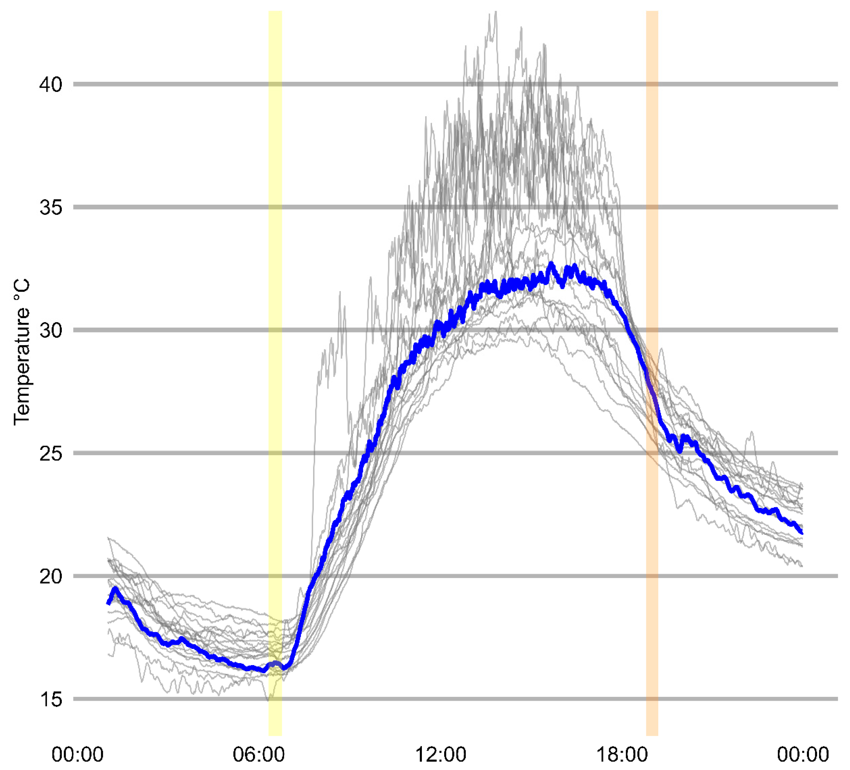
3.3. “Hot Sunny” Example

While the long-term trends averaged over the study period largely follow a priori expectations for land use change, case studies of individual days are particularly interesting. Nighttime conditions, or generally cloudy daytime conditions, see sensors revert to their land-cover-driven trends. However, daytime, sunny conditions can lead to significant differences in temperatures and humidities across our small study area. One example is 24 September. The expected 30-year climatology in Mobile, Alabama is a daily high temperature of 30.5 °C and a low of 21.1 °C. On this particular day, conditions were several degrees warmer and dewpoints were relatively low with a light breeze for most of the day with few clouds in the sky for the majority of the day. However, the various land covers across campus showed a complex story.

Figure 3 displays the twenty-one stations included in the study. The blue line represents the readings from the USA Mesonet. Temperatures recorded at the Mesonet station never exceeded 32.6 °C (at 15:26, local time), yet the hottest temperature at this exact time across all stations was located at an urban station—41.3 °C, and the coolest temperature was at a natural station at 29.2 °C, or a 12.1° range across the 1.5 square miles of campus. Yet the global maximum temperature was 42.85 °C, recorded approximately two hours earlier at 13:38, local time, at a station classified as natural (located on a footbridge overlooking Three Mile Creek in minimal canopy cover for most of the early afternoon). The range of temperatures at this point across campus was 13.6°, while the USA Mesonet registered a temperature of 31.8 °C. Furthermore, 24 September was the warmest day in the study period, yet there were more than a dozen other days that had similar differences in temperature across campus in daytime sunny conditions.

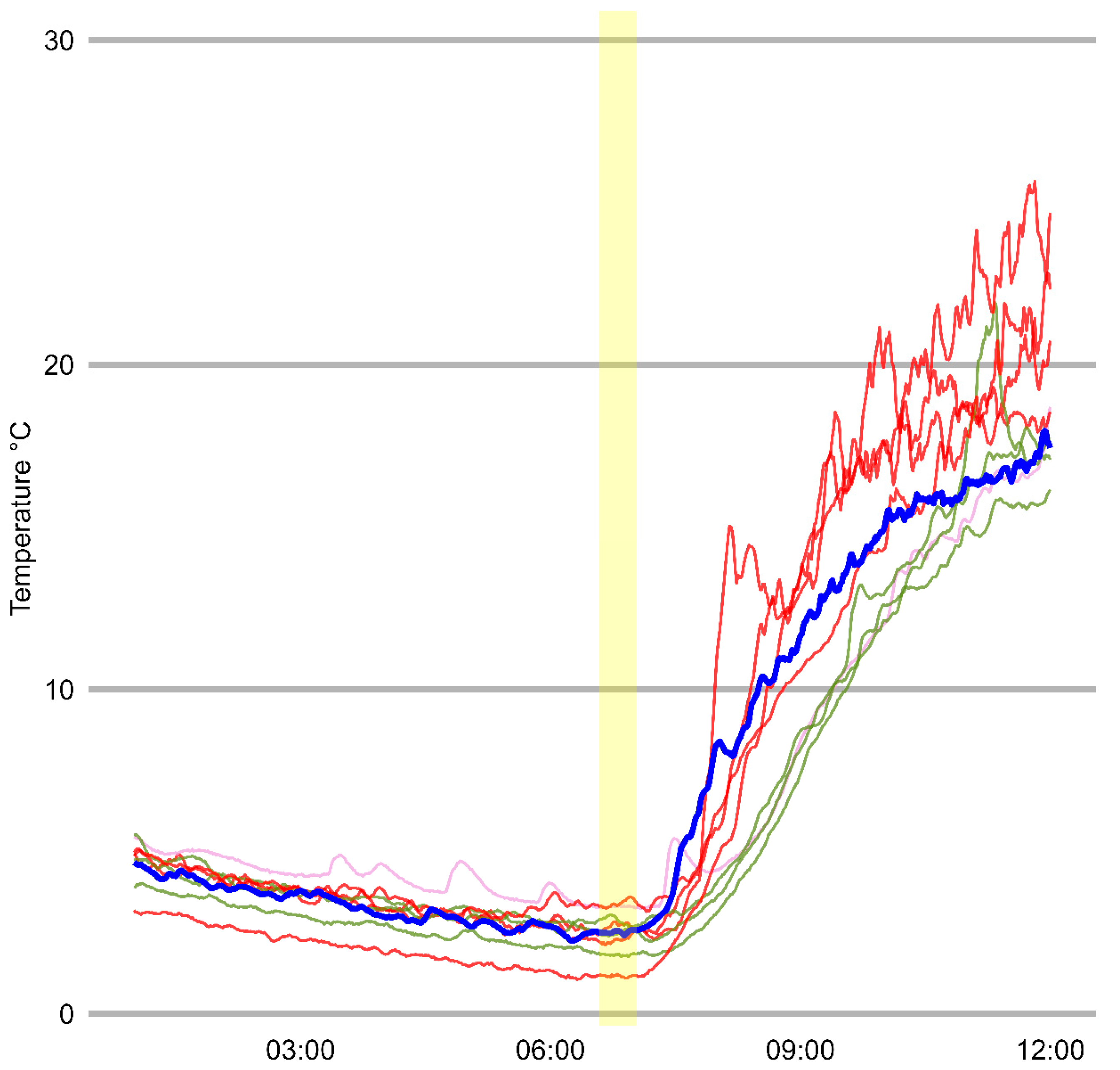
3.4. “Early Fall Chill” Example

The Gulf Coast of the United States is known far more for warm rather than cold temperatures, but mid-late October had a rare early chance to see differences in temperature across the study area during abnormally cool temperatures on 20 October. Temperatures were significantly below the climatological average with nighttime temperatures dropping near freezing. Conditions in the early morning hours of 20 October saw clear skies, a light breeze, and instances of localized frost—a rarity for this time of year for the region.

Figure 4 displays the temperatures from each station and the USA Mesonet Station from the hours of midnight to 8:00, local time. Temperatures varied by approximately five degrees Fahrenheit for most of the night with occasional minor fluctuations, but from the point of civil twilight beginning at 6:33 local time until well past sunrise, one can see many differences. The Mesonet began warming up nearly after the moment of daybreak, several hours before the natural and landscaped stations. The urban stations warm up rapidly, beginning at approximately the same time and at the same rate, though it continues the warming trend until it reaches a temperature of nearly 20 °C. This is likely due to the general lack of shading at all but one urban station in the morning hours. By noon, temperatures varied by more than 10 °C between the warmest and coldest stations.

The nighttime temperatures at the natural and landscaped stations appear, on the whole, to be of equal temperature or warmer than the mesonet and urban stations, though this is likely due to canopy cover above the stations. These stations then warm up slower than the other stations likely for the same reason: presence of canopy cover and a lack of direct sun. The implications here matter for decision making on an individual scale and on a larger scale, which will be discussed in the next section.

4. Discussion

4.1. Implications for Atmospheric Sciences

The need for studies of the urban microclimate is needed for a world that is seeing rising temperatures and more people moving to or being born into urban spaces. The previous studies have shown that temperatures can vary immensely over small spaces, but many of these studies—though highly useful to the existing literature—were limited by spatiotemporal resolution or surface cover types [49,50]. This study sought to place stations in situ as a measure of the environment that people (and things) naturally interact with on a daily basis in such an area. While the University of South Alabama’s campus should not be compared directly to great megalopoli of the world in terms of population density or urban landscape, it does feature a wide array of potential land covers. This study found that microclimates can lead to very large differences in atmospheric conditions at specific points. The past research has shown that, in essence, “Mesoclimates endure the averages, Microclimates endure the extremes” and not just in an urban setting [18]. This study supports that idea as the 20 sensors plus the USA Mesonet station could find as much as a 13 °C difference in temperature across campus during sunny, daytime conditions. During nighttime, temperature differences still existed—as high as 6 degrees at times. This is a clear example of the canopy layer—urban heat island effect and its components driving temperatures in different conditions. Long term average differences between various land covers are comparable to other studies [51,52]; however, there is a higher level of smaller timescale variability likely due to canopy cover differences and the late-summer, subtropical conditions of this study, though results were very similar to results found with an urban microclimate network in a heat-wave example in Berlin, DE in Fenner et al. 2024 [53].

Yet, mesoscale weather networks simply cannot pick up such differences over space. Among other reasons for this, mesoscale networks are not designed to record such data. Mesoscale networks place stations in idealized locations for scientific replicability, and rightly so. These observation networks are the backbone of the entire field of atmospheric science, and it is imperative to record data in this way. Moreover, it is not feasible to place weather stations on street signs, under trees, or other locations due to cost, maintenance, and a number of other logistical reasons. This study is not an attempt to suggest that this should be carried out. Rather, we show just how much temperatures (and humidities) vary over relatively small spaces that, in this case, had one mesoscale station located within the network. Observing and analyzing data at the mesoscale shows only a glimpse of just how complex atmospheric conditions can be over complex terrain.

The disconnect between the mesoscale and microscale is an idea that has existed for some time and not just in Meteorology or Climatology [54,55]. This study, in fact, reflects the geographic question of spatiotemporal resolution and the modifiable areal unit problem (MAUP) [56]. One may observe something at one scale and see something completely different at another [57]. In this case, a Mesoscale Network would register a temperature of 30 °C, yet a microscale network may find temperatures 10° higher or 5° lower at the same moment. While a microscale network is not feasible for all locations or times, it can give a view into just how variable the world can be when “zoomed in” a little further. This, then, has implications for society.

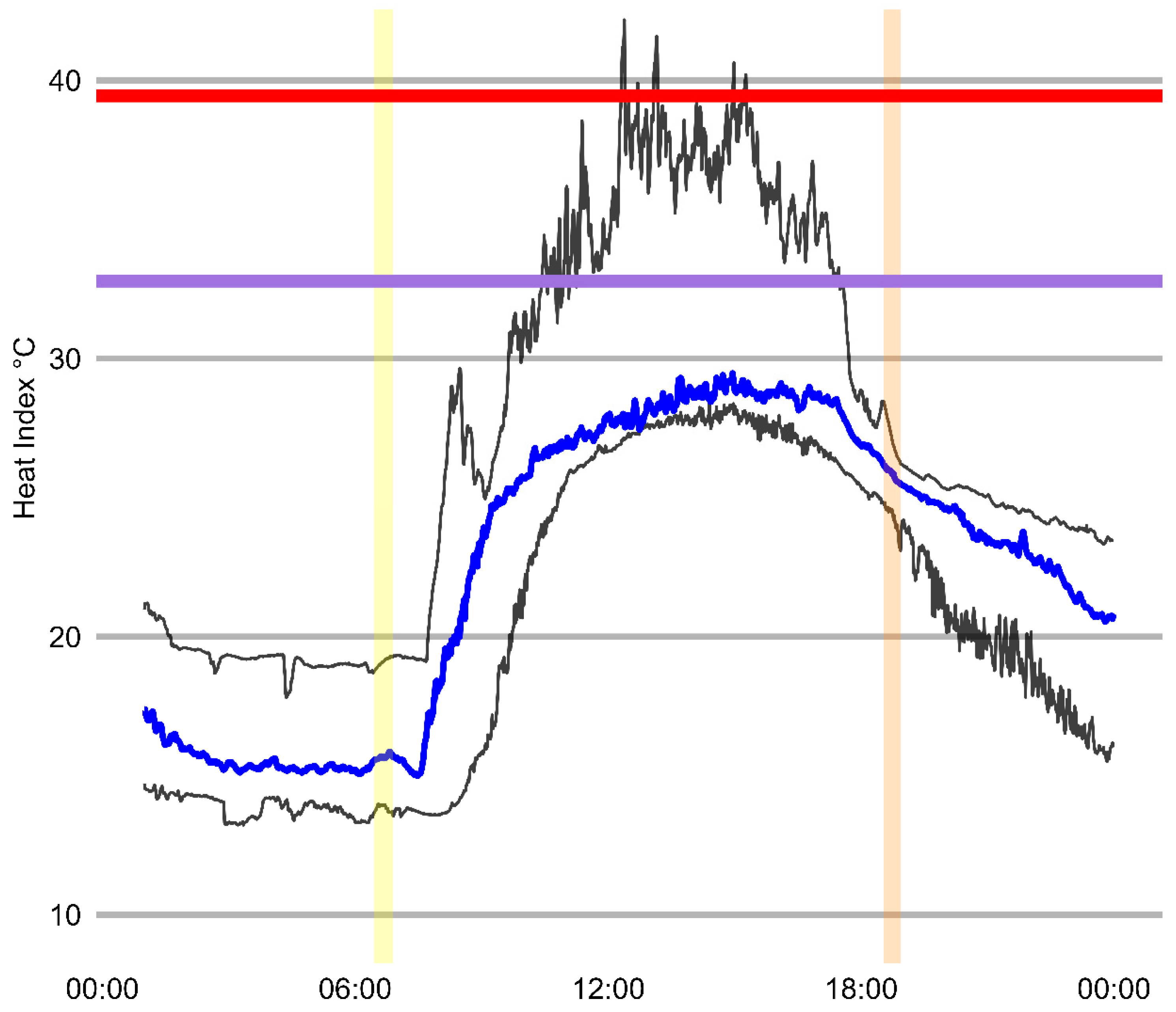
4.2. Implications for Society (Heat Index Example)

This paper sought to compare the microscale network of in situ sensors to the mesoscale station. Not only did that mesoscale station act as the “control” in the experiment, one could see the mesoscale station as the data that a person checking publicly available weather data might use. The question of how the public utilizes weather data and understands complex concepts such as thermal indices are still being studied, but most will use this data to make decisions in some capacity. Whether a data user checks their preferred website or news source for the daily high or low temperature or someone opens their mobile phone app to see the current conditions, decisions can be made from the obtained data. Daily plans, what to wear, what to eat, should the garden be watered, is it worth taking the bus or riding a bike—it is not difficult to imagine the spectrum of decisions that can be made by having these data at the ready. Yet, these data come directly or are processed from the mesoscale.

One could say that “we make decisions at the mesoscale” because we have our data collected at such a scale, yet we “live in a microclimate world” because microclimates are the actual environments that someone must encounter when they enter the natural environment. In the “Early Fall Chill” example (Figure 4), temperatures hovered above freezing for several hours, and the sensors showed temperatures with a range of approximately 3 to 4 degrees. Additionally, the stations warmed up after sunrise at different rates. A decision to cover plants in a garden or a fruit tree would have been difficult to make, and not covering plants in the campus community garden that morning could have proven costly as frost was reported on campus. While this is circumstantial evidence from the study area and time, it does confirm previous microclimatic studies. Checking a weather app would have shown temperatures hovering around 2 °C then warming up quickly to 10 °C by 7:00 am local time—yet the landscaped and natural stations did not warm to 10 °C until 10:00. In a town nicknamed the “Azalea City” for the vast number of azalea flowering plants across Mobile and the flower nurseries to the west of town, a difference of even one or two-degrees temperature coupled with longer exposure to these low temperatures can cost millions of dollars if the wrong decision is made.

This has impacts beyond agriculture and floriculture. The State of Alabama has a storied history with sports at the amateur level, notably high school and college level American football [58]. High levels of competition and fierce rivalries are part of society in the region, even among those not interested in sport. Due to the state being located in the American Southeast, and the fact that football practices begin, typically, in July and August, the Alabama High School Athletic Association (AHSAA) has regulated practices such that coaches and student athletes at the high school level must consider heat index calculations when determining practice intensity [59]. Below 91 °F (32.8 °C), practices can occur normally. Between heat indices of 91 °F and 103 °F (39.4 °C), practices must be limited to two hours in length with minimal pads (helmet and shoulder pads only) with certain rules for the number of breaks that must be taken. Above a 103 °F heat index, practices are limited to one hour, helmets are the only padding required, and 20-min breaks must be taken. Above 126 °F (52.2 °C) heat index, practice cannot be held outside. One must also rely on a coach that is utilizing the nearby weather data to make such a decision and that they will ultimately follow these rules in the name of player safety. Sadly, this has not always been the case in recent times [60,61].

Our study considered this when calculating the heat index at all stations for the study time. Specifically, 7 October was a climatologically average day in terms of temperature, humidity, and other atmospheric variables. It is also in the middle of high school football season in the region. Figure 5 shows the thresholds previously mentioned, as well as the maximum HI across the sensors, lowest HI, and the HI calculated specifically at the Mesonet. It should first be noted that the range of HI values varies greatly between the highest and lowest values calculated at our stations as the day progresses. Second, the maximum reading of any of the sensors was nearly always above the 91 °F (32.8 °C) threshold (purple line) from approximately 9 a.m. to 5 p.m. However, perhaps most concerning is that the Mesonet station never registered above the 91 °F threshold during the entire 24-h period. In fact, the Mesonet was the station reading one of the lowest HI values for several hours in the afternoon of 7 October, while some sensors registered above the 103 °F (39.4 °C) threshold (red line) at times that afternoon. A coach using their phone to inspect the heat index would not have had any reason to take the required precautions at any time during that day. Player safety would not be guaranteed in this instance. It should be noted that this was only for 7 October, while similar scenarios occurred on other days in the study period. Considering the evidence found in this study, it may be prudent for football teams or associations to include a weather sensor, such as a NetAtmo sensor (as used in Chapman et al. 2017 [36] or van der Linden 2023 [62]) along with the first aid equipment. The cost of sensors will continue to become lower, and the sport of American football is typically a costly, equipment-heavy venture, so it could reasonable to include a sensor to calculate heat index on a playing surface in the name of player safety.

4.3. Implications for Urban Microclimates

Having such a vast range of temperatures over a relatively small, urbanized area has implications for cities in the present and in the future. Urban planning [64], architecture [65], real estate [66], engineering [67], economics [68], and policy are all fields that could take note of this study as these fields are already concerned with the urban heat island and its effects on people living within it. However, in a world where warmer temperatures are becoming more frequent, and heat waves are becoming longer [69], more intense [70], and more deadly [71], these microclimatic differences need further study.

Decision making does not need to be limited just to the small scale, as presented in the previous subsection. When either expanding or updating urban spaces, extreme temperatures and other extreme meteorological conditions need to be considered. Planting greenspaces and adapting energy grids is one method of doing this [72], but progress is slow. Hotter days, warmer nights, higher energy costs [73], and the logistics of distributing resources in these urban spaces is one of several problems future urban spaces will need to consider. Going beyond the field of atmospheric sciences, city developers from all fields will continue to need to find solutions as more people move to urban spaces in the coming decades. Just as with most issues connected to anthropogenic climate change, the cost of a delayed response is far higher than starting to confront the issue today [74].

5. Conclusions

The goal of this student-driven study was to find just how much temperatures varied on a microscale compared to what one would find on a mesoscale. Using the University of South Alabama’s campus as a proxy for a diverse urban space allowed the authors to explore the effects of land cover and aspect and to show an example of the potential of how such data could factor into decision making.

As previously mentioned, this study does not present itself as a feasible alternative to replacing mesoscale networks of meteorological datasets. Rather, it was implemented to show just how much variability existed around a station for such a network. As shown in the previous sections, temperatures can vary by as much as 13 °C at the same minute over the study area, and the implications for decision making at different scales are large.

Future research will include an expanded dataset over a longer period of time in slightly different locations on the university campus. The authors believe that the diversity of land covers studied on campus was robust, but there were some covers that were not studied only because the study only used twenty sensors (plus the Mesonet station). Additionally, placing more sensors on different aspect bearings would have been interesting, yet it should be noted that the University of South Alabama’s campus is relatively flat. Aspect can have a larger impact at higher latitudes or when there is more topographical change, two issues that cannot be addressed on our campus. Replicating this study at a university 15° of latitude north—at 45° N—could yield results that show that aspect has a larger role in temperature differences. A concurrent study is in an ecologically remote area in the Galápagos Islands, located effectively at the Equator (0°), with the same experimental design and goals in mind, though the focus is less on urbanized spaces. Overall, the authors believe they have only just started on this path of studying microclimates at a very high spatiotemporal resolution with sensors sitting in situ to serve as a study of a realistic environment compared to the idealized surroundings of a mesoscale weather station. The goal is to show just how diverse atmospheric conditions can be when “zooming in” across certain areas. The results so far show just how complex our environment can be, and the implications are numerous.

References

1. Blum, A. The Weather Machine: A Journey Inside the Forecast; Ecco: Manhattan, NY, USA, 2019; 224p. [Google Scholar]
2. Muñoz-Esparza, D.; Kosović, B.; Mirocha, J.; van Beeck, J. Bridging the transition from mesoscale to microscale turbulence in numerical weather prediction models. Bound.-Layer Meteorol. 2014, 153, 409–440. [Google Scholar] [CrossRef]
3. Schultze, S.R.; Sabbatini, P. Implications of a climate-changed atmosphere on cool-climate viticulture. J. Appl. Meteorol. Climatol. 2019, 58, 1141–1153. [Google Scholar]
4. Wiersema, D.J.; Lundquist, K.A.; Chow, F.K. Mesoscale to microscale simulations over complex terrain with the immersed boundary method in the Weather Research and Forecasting Model. Mon. Weather Rev. 2020, 148, 577–595. [Google Scholar]
5. Haupt, S.E.; Kosovic, B.; Shaw, W.; Berg, L.K.; Churchfield, M.; Cline, J.; Draxl, C.; Ennis, B.; Koo, E.; Kotamarthi, R.; et al. On bridging a modeling scale gap: Mesoscale to microscale coupling for wind energy. Bull. Am. Meteorol. Soc. 2019, 100, 2533–2550. [Google Scholar]
6. Schultze, S.R.; Campbell, M.N.; Walley, S.; Pfeiffer, K.; Wilkins, B. Exploration of sub-field microclimates and winter temperatures: Implications for precision agriculture. Int. J. Biometeorol. 2021, 65, 1043–1052. [Google Scholar] [PubMed]
7. Portela, J.R.D.; Galvez, G.H.; Hernandez-Escobedo, Q.; Flores, R.S.; Martínez, O.S.; Danguillecourt, O.L.; de Paz, P.L.; Perea-Moreno, A.-J. Microscale Wind Assessment, Comparing Mesoscale Information and Observed Wind Data. Sustainability 2022, 14, 11991. [Google Scholar] [CrossRef]
8. World Bank. Urban Development Overview. 2023. Available online: https://www.worldbank.org/en/topic/urbandevelopment/overview (accessed on 20 July 2023).
9. Chow, F.K.; Schär, C.; Ban, N.; Lundquist, K.A.; Schlemmer, L.; Shi, X. Crossing multiple gray zones in the transition from mesoscale to microscale simulation over complex terrain. Atmosphere 2019, 10, 274. [Google Scholar] [CrossRef]
10. Piroozfar, P.; Farr, E. Urban Heat Mitigation: Current and Future Trends. In The Routledge Companion to Ecological Design Thinking; Routledge: Abingdon, UK, 2022; pp. 150–160. [Google Scholar]
11. Javanroodi, K.; Nik, V.M.; Giometto, M.G.; Scartezzini, J.L. Combining computational fluid dynamics and neural networks to characterize microclimate extremes: Learning the complex interactions between meso-climate and urban morphology. Sci. Total Environ. 2022, 829, 154223. [Google Scholar] [CrossRef]
12. Burian, S.J.; Shepherd, J.M. Effect of urbanization on the diurnal rainfall pattern in Houston. Hydrol. Process. Int. J. 2005, 19, 1089–1103. [Google Scholar]
13. Zhou, Y.; Shepherd, J.M. Atlanta’s urban heat island under extreme heat conditions and potential mitigation strategies. Nat. Hazards 2010, 52, 639–668. [Google Scholar]
14. Chatterjee, U.; Majumdar, S. Impact of land use change and rapid urbanization on urban heat island in Kolkata city: A remote sensing based perspective. J. Urban Manag. 2022, 11, 59–71. [Google Scholar] [CrossRef]
15. Oke, T.R. City Size and Urban Heat Island. Atmos. Environ. 1973, 7, 769–779. [Google Scholar] [CrossRef]
16. Ashcroft, M.B.; Gollan, J.R. Fine-resolution (25 m) topoclimatic grids of near-surface (5 cm) extreme temperatures and humidities across various habitats in a large (200 × 300 km) and diverse region. Int. J. Climatol. 2012, 32, 2134–2148. [Google Scholar]
17. Barry, R.G.; Blanken, P.D. Microclimate and Local Climate; Cambridge University Press: Cambridge, UK, 2016. [Google Scholar]
18. Fiebrich, C.A.; Crawford, K.C. Automation: A Step toward Improving the Quality of Daily Temperature Data Produced by Climate Observing Networks. J. Atmos. Ocean. Technol. 2009, 26, 1246–1260. [Google Scholar] [CrossRef]
19. Cassano, J.J. Weather Bike: A Bicycle-Based Weather Station for Observing Local Temperature Variations. Bull Am. Meteor. Soc. 2014, 95, 205–209. [Google Scholar]
20. Oke, T.R. Boundary Layer Climates; Routledge: Abingdon, UK, 2002; 435p. [Google Scholar]
21. Oke, T.R. The energetic basis of the urban heat island. Q. J. R. Meteorol. Soc. 1982, 108, 1–24. [Google Scholar] [CrossRef]
22. Mills, G. Luke Howard and the climate of London. Weather 2008, 63, 153–157. [Google Scholar] [CrossRef]
23. Howard, L. The Climate of London: Deduced from Meteorological Observations; Cambridge University Press: Cambridge, UK, 2012; Volume 1. [Google Scholar]
24. Stewart, I.D. Why should urban heat island researchers study history? Urban Clim. 2019, 30, 100484. [Google Scholar]
25. Hsu, S.I. Variation of an urban heat island in Phoenix. Prof. Geogr. 1984, 36, 196–200. [Google Scholar] [CrossRef]
26. Brazel, A.; Gober, P.; Lee, S.J.; Grossman-Clarke, S.; Zehnder, J.; Hedquist, B.; Comparri, E. Determinants of changes in the regional urban heat island in metropolitan Phoenix (Arizona, USA) between 1990 and 2004. Clim. Res. 2007, 33, 171–182. [Google Scholar] [CrossRef]
27. Parlow, E.; Vogt, R.; Feigenwinter, C. The urban heat island of Basel—Seen from different perspectives. DIE ERDE 2014, 145, 96–110. [Google Scholar]
28. Oke, T.R.; Mills, G.; Christen, A.; Voogt, J.A. Urban Climates; Cambridge University Press: Cambridge, UK, 2017. [Google Scholar]
29. Almeida, C.R.D.; Teodoro, A.C.; Gonçalves, A. Study of the urban heat island (UHI) using remote sensing data/techniques: A systematic review. Environments 2021, 8, 105. [Google Scholar] [CrossRef]
30. Balchin, W.G.V.; Pye, N. A micro-climatological investigation of bath and the surrounding district. Q. J. R. Meteorol. Soc. 1947, 73, 297–323. [Google Scholar]
31. Balchin, W.G.V.; Pye, N. Local rainfall variations in Bath and the surrounding district. Q. J. R. Meteorol. Soc. 1948, 74, 361–378. [Google Scholar]
32. Balchin, W.G.V.; Pye, N. Observations on local temperature variations and plant response. J. Ecol. 1950, 38, 345–353. [Google Scholar]
33. Jha, M.; Marpu, P.R.; Chau, C.K.; Armstrong, P. Design of sensor network for urban micro-climate monitoring. In Proceedings of the 2015 IEEE First International Smart Cities Conference (ISC2), Guadalajara, Mexico, 25–28 October 2015; pp. 1–4. [Google Scholar]
34. Chapman, L.; Bell, C.; Bell, S. Can the crowdsourcing data paradigm take atmospheric science to a new level? A case study of the urban heat island of London quantified using Netatmo weather stations. Int. J. Climatol. 2017, 37, 3597–3605. [Google Scholar] [CrossRef]
35. Ramakreshnan, L.; Aghamohammadi, N.; Fong, C.S.; Ghaffarianhoseini, A.; Wong, L.P.; Sulaiman, N.M. Empirical study on temporal variations of canopy-level Urban Heat Island effect in the tropical city of Greater Kuala Lumpur. Sustain. Cities Soc. 2019, 44, 748–762. [Google Scholar]
36. Kalogeropoulos, G.; Dimoudi, A.; Toumboulidis, P.; Zoras, S. Urban Heat Island and Thermal Comfort Assessment in a Medium-Sized Mediterranean City. Atmosphere 2022, 13, 1102. [Google Scholar] [CrossRef]
37. WMO. Guidance on Measuring, Modelling and Monitoring the Canopy Layer Urban Heat Island (CL-UHI); WMO-No. 1292; WMO: Geneva, Switzerland, 2023. [Google Scholar]
38. Schultze, S.R.; Martin, J.; West, K.; Swinea, L.; Linzmeier, B.J. Urban microclimates in action! High resolution temperature and humidity differences across diverse urban terrain. In Proceedings of the Poster for 2022 American Geophysical Union Annual Meeting, Chicago, IL, USA, 12–16 December 2022. [Google Scholar]
39. Goolsby, I.; Martin, J.; West, K.; Swinea, L.; Linzmeier, B.J.; Schultze, S.R. Urban microclimates in action! High resolution temperature and humidity differences across diverse urban terrain. In Proceedings of the Poster for 2024 American Association of Geographers Annual Meeting, Honolulu, HI, USA, 16–20 April 2024. [Google Scholar]
40. Köppen, W. Versuch einer Klassifikation der Klimate, vorzugsweise nach ihren Beziehungen zur Pflanzenwelt. Geogr. Z. 1900, 6, 593–611. [Google Scholar]
41. Geiger, R.; Aron, R.H.; Todhunter, P. The Climate Near the Ground; Rowman & Littlefield: Lanham, MD, USA, 2009. [Google Scholar]
42. Svoboda, M.; LeComte, D.; Hayes, M.; Heim, R.; Gleason, K.; Angel, J.; Rippey, B.; Tinker, R.; Palecki, M.; Stooksbury, D.; et al. The drought monitor. Bull. Am. Meteorol. Soc. 2002, 83, 1181–1190. [Google Scholar]
43. US Drought Monitor. Mobile (MOB) NWS WFO Drought Time Series Graph. 2023. Available online: https://droughtmonitor.unl.edu/dmData/Timeseries.aspx (accessed on 20 July 2023).
44. Dewitz, J. National Land Cover Database (NLCD) 2019 Products [Data Set]; U.S. Geological Survey; Earth Resources Observation and Science (EROS) Center: Sioux Falls, SD, USA, 2021.
45. Stewart, I.D.; Oke, T.R. Local climate zones for urban temperature studies. Bull. Am. Meteorol. Soc. 2012, 93, 1879–1900. [Google Scholar] [CrossRef]
46. Kimball, S.; Montalvo, C.; Mulekar, M. Evaluating temperature measurements of the iMET-XQ, in the field, under varying atmospheric conditions. Atmosphere 2020, 11, 335. [Google Scholar] [CrossRef]
47. R Core Team. R: A Language and Environment for Statistical Computing; R Foundation for Statistical Computing: Vienna, Austria, 2022. [Google Scholar]
48. Wickham, H.; Averick, M.; Bryan, J.; Chang, W.; McGowan, L.D.; François, R.; Grolemund, G.; Hayes, A.; Henry, L.; Hester, J.; et al. Welcome to the tidyverse. J. Open Source Softw. 2019, 4, 1686. [Google Scholar] [CrossRef]
49. Elmarakby, E.; Khalifa, M.; Elshater, A.; Afifi, S. Tailored methods for mapping urban heat islands in Greater Cairo Region. Ain Shams Eng. J. 2022, 13, 101545. [Google Scholar] [CrossRef]
50. Cureau, R.J.; Pigliautile, I.; Pisello, A.L. Seasonal and diurnal variability of a water body’s effects on the urban microclimate in a coastal city in Italy. Urban Clim. 2023, 49, 101437. [Google Scholar] [CrossRef]
51. Fortuniak, K.; Kłysik, K.; Wibig, J. Urban–rural contrasts of meteorological parameters in Łódź. Theor. Appl. Climatol. 2006, 84, 91–101. [Google Scholar] [CrossRef]
52. Fenner, D.; Meier, F.; Scherer, D.; Polze, A. Spatial and temporal air temperature variability in Berlin, Germany, during the years 2001–2010. Urban Clim. 2014, 10, 308–331. [Google Scholar] [CrossRef]
53. Fenner, D.; Christen, A.; Grimmond, S.; Meier, F.; Morrison, W.; Zeeman, M.; Barlow, J.; Birkmann, J.; Blunn, L.; Chrysoulakis, N.; et al. urbisphere-Berlin Campaign: Investigating Multiscale Urban Impacts on the Atmospheric Boundary Layer. Bull. Am. Meteor. Soc. 2024, 105, E1929–E1961. [Google Scholar] [CrossRef]
54. Clark, W.A.V. Definitive theories or alternative perspectives: Comments on urban geography and social theory. Urban Geogr. 1988, 9, 252–254. [Google Scholar] [CrossRef]
55. Qi, L.; Chantler, M.J.; Siebert, J.P.; Dong, J. The joint effect of mesoscale and microscale roughness on perceived gloss. Vis. Res. 2015, 115, 209–217. [Google Scholar] [CrossRef]
56. Wong, D.W. The modifiable areal unit problem (MAUP). In WorldMinds: Geographical Perspectives on 100 Problems: Commemorating the 100th Anniversary of the Association of American Geographers 1904–2004; Springer: Dordrecht, The Netherlands, 2004; pp. 571–575. [Google Scholar]
57. Dark, S.J.; Bram, D. The modifiable areal unit problem (MAUP) in physical geography. Prog. Phys. Geogr. 2007, 31, 471–479. [Google Scholar] [CrossRef]
58. ESPN. Alabama—Auburn Football Game, 2013, Box Score. 2013. Available online: https://www.espn.com/college-football/boxscore/_/gameId/333340002 (accessed on 24 July 2023).
59. AHSAA. Heat Index Exercise Restrictions. 2023. Available online: https://www.ahsaa.com/Portals/0/PDF%27s/AHSAA/Safety/2024%20HEAT%20INDEX%20EXERCISE%20RESTRICTIONS.pdf?ver=9iIB3gxVgff67Dkl8gpdSg%3D%3D&timestamp=1716899684958 (accessed on 21 July 2023).
60. Francis, K.; Feinstein, R.; Brasher, J. Heat illness in football players in Alabama. Ala. Med. J. Med. Assoc. State Ala. 1991, 60, 10–14. [Google Scholar]
61. WSFA. High School Football Player Dies After Collapsing from Heatstroke, Family Says. 2021. Available online: https://www.wsfa.com/2021/08/12/high-school-football-player-dies-after-collapsing-heatstroke-family-says/ (accessed on 23 July 2023).
62. van der Linden, L.; Hogan, P.; Maronga, B.; Hagemann, R.; Bechtel, B. Crowdsourcing air temperature data for the evaluation of the urban microscale model PALM—A case study in central Europe. PLoS Clim. 2023, 2, e0000197. [Google Scholar]
63. Rothfusz, L.P. The Heat Index Equation (or, More Than You Ever Wanted to Know About Heat Index); National Oceanic and Atmospheric Administration, National Weather Service, Office of Meteorology: Fort Worth, TX, USA, 1990.
64. Allen-Dumas, M.R.; Rose, A.N.; New, J.R.; Omitaomu, O.A.; Yuan, J.; Branstetter, M.L.; Sylvester, L.M.; Seals, M.B.; Carvalhaes, T.M.; Adams, M.B.; et al. Impacts of the morphology of new neighborhoods on microclimate and building energy. Renew. Sustain. Energy Rev. 2020, 133, 110030. [Google Scholar]
65. Montelpare, S.; D’Alessandro, V.; Lops, C.; Costanzo, E.; Ricci, R. A Mesoscale-Microscale approach for the energy analysis of buildings. J. Phys. Conf. Ser. 2019, 1224, 012022. [Google Scholar]
66. Hsu, A.; Sheriff, G.; Chakraborty, T.; Manya, D. Disproportionate exposure to urban heat island intensity across major US cities. Nat. Commun. 2021, 12, 2721. [Google Scholar] [CrossRef]
67. Golden, J.S. The built environment induced urban heat island effect in rapidly urbanizing arid regions–a sustainable urban engineering complexity. Environ. Sci. 2004, 1, 321–349. [Google Scholar]
68. Marks, D.; Connell, J. Unequal and unjust: The political ecology of Bangkok’s increasing urban heat island. Urban Stud. 2023, 61, 2887–2907. [Google Scholar]
69. Meehl, G.A.; Tebaldi, C. More intense, more frequent, and longer lasting heat waves in the 21st century. Science 2004, 305, 994–997. [Google Scholar]
70. Stillman, J.H. Heat waves, the new normal: Summertime temperature extremes will impact animals, ecosystems, and human communities. Physiology 2019, 34, 86–100. [Google Scholar]
71. Pascal, M.; Lagarrigue, R.; Laaidi, K.; Boulanger, G.; Denys, S. Have health inequities, the COVID-19 pandemic and climate change led to the deadliest heatwave in France since 2003? Public Health 2021, 194, 143–145. [Google Scholar] [CrossRef] [PubMed]
72. Piroozmand, P.; Mussetti, G.; Allegrini, J.; Mohammadi, M.H.; Akrami, E.; Carmeliet, J. Coupled CFD framework with mesoscale urban climate model: Application to microscale urban flows with weak synoptic forcing. J. Wind Eng. Ind. Aerodyn. 2020, 197, 104059. [Google Scholar] [CrossRef]
73. Errebai, F.B.; Strebel, D.; Carmeliet, J.; Derome, D. Impact of urban heat island on cooling energy demand for residential building in Montreal using meteorological simulations and weather station observations. Energy Build. 2022, 273, 112410. [Google Scholar] [CrossRef]
74. Manzanedo, R.D.; Manning, P. COVID-19: Lessons for the climate change emergency. Sci. Total Environ. 2020, 742, 140563. [Google Scholar] [CrossRef] [PubMed]
Figure 1. Map of campus microsensor sites, plus USA Mesonet, classified by land cover and accompanied with NLCD land use class.
Atmosphere 16 00416 g001
Figure 2. Average temperature in °C by aspect for all 21 stations included in the study from 1 October to 14 October.
Atmosphere 16 00416 g002
Figure 3. Temperature graph, in °C, for all 21 stations included in the study for 24 September for each minute. Sunrise and sunset times are added as lines. Blue line is USA Mesonet and grey lines are individual stations. Vertical yellow and orange bars are sunrise and sunset times.
Atmosphere 16 00416 g003
Figure 4. Temperature in °C at all recording sensors classified by color (red = urban, plum = landscaped, green = natural) and the USA Mesonet (in blue) in the A.M. hours of 20 October. Sunrise time in yellow is highlighted.
Atmosphere 16 00416 g004
Figure 5. Heat index calculated, as from Rothfusz 1990 [63], in °C from 21 stations for 7 October with maximum, minimum for all stations, along with the USA Mesonet calculated HI, and the two temperature thresholds (32.8 °C in purple, 39.4 °C in red) according to ASHAA regulations for American football practices. Sunrise (yellow)and sunset (orange) times are highlighted.
Atmosphere 16 00416 g005