Abstract
This study explores rainfall variability and trends in the Enkangala Escarpment of South Africa using station data from 1972 to 2022 (51 years). The coefficient of variation (CV) is indicative of pronounced inter-annual variability in seasonal rainfall totals across the region. The trend-free pre-whitening Mann–Kendall (TFPWMK) test and innovative trend analysis (ITA) were used to determine the presence of monotonic trends in the station records, despite the pronounced inter-annual variability in the time series. Sen’s slope estimator was used to quantify the magnitude of the trends. For a given season, the ITA test, in general, allocates local statistical significance to the time series for more stations compared to the TFPWMK test. For winter, spring and summer, there is spatial coherency of decreasing rainfall trends across the Enkangala Escarpment. These trends also exhibit local significance for spring at most stations, and are indicative of less favorable growing conditions for crops during this season. Reduced spring rainfall is likely to also translate to later planting dates (a shorter growing season) and a longer burning season. Trends for autumn are generally weak and lack in local statistical significance or spatial coherency.
1. Introduction
South Africa’s Great Escarpment stretches over almost 1000 km from the eastern parts of the Eastern Cape in the south to the Limpopo Province in the north. The escarpment substantially shapes the climate of South Africa’s summer rainfall region, inducing high rainfall totals over and toward the east of the mountains while casting a rain shadow over the interior regions to the west. The Maloti-Drakensberg is the highest part of the Great Escarpment and is the best studied from a climate science perspective. This is due to the pronounced climate change this region has undergone since the Last Glacial Maximum (LGM), as deduced from proxy records and model reconstructions [1,2], and concerns about the impacts of future climate change [3]. In particular, the Maloti-Drakensberg gives rise to the rivers that supply South Africa’s mega-dam region with water, and there are grave concerns about climate change bringing more severe multi-year droughts to this region, threatening South Africa’s water security [4,5]. Less studied is climate variability and change over the part of the escarpment to the north, namely, the Enkangala Escarpment, along the north-western border of South Africa’s KwaZulu Natal Province. This is a relatively low part of the escarpment, with altitudes between 1200 and 1700 m [3]. It is a part of the escarpment with local importance rather than being important from a national water security perspective, in the sense that it supports rainfed and irrigated maize and citrus agriculture, as well as livestock farming [3]. The grasslands of this region are rich in biodiversity, and both the Thukela and Phongolo rivers have their origins in the Enkangala Escarpment [3]. The super El Niño event of 2015/16 brought severe drought to the Enkangala Escarpment and, in combination with some evidence of systematic negative trends in rainfall in this region [6], raised questions about the impacts of future climate change. Here, we explore whether systematic trends in rainfall can be detected in the Enkangala Escarpment.
The El Niño Southern Oscillation (ENSO) had a pronounced impact on inter-annual climate variability over eastern South Africa [7], with regional modes of variability such as the subtropical South Indian Ocean dipole playing a secondary role [8]. Rainfall over the Enkangala Escarpment is largely of a convective nature, with most rain occurring in the form of thunderstorms embedded within tropical-temperate cloud bands [9]. Ridging high-pressure systems play an important role in terms of the transport of low-level moisture into the region [10], sometimes generating favorable conditions for tropical lows to bring heavy falls of rain into the area [11]. Periods of pronounced drought in the region are characterised by the absence or reduced frequency of these rainfall-producing systems because of the prevailing subsidence occurring under the subtropical high-pressure systems that induce periods of summer drought [12].
The Intergovernmental Panel on Climate Change (IPCC), in its Assessment Report Six (AR6), reported decreasing rainfall trends over the large region of ‘eastern southern Africa’, which includes eastern South Africa [4]. This is consistent with the rainfall trend analysis of a number of studies that are indicative of decreasing rainfall totals and the increasing occurrence of drought in eastern South Africa [13,14]. The IPCC also made the assessment that extreme precipitation events have been increasing in recent decades in eastern southern Africa, with South African-based studies indicative of such trends also occurring over the encompassed Enkangala Escarpment [15].
Across the African continent, rainfed agriculture is vulnerable to climate change impacts, especially in the context of a lack of adaptation capacity in water-stressed regions [16,17,18]. This also holds true for the Enkangala Escarpment. Consequently, this study aims to identify the potential presence of long-term rainfall trends over the Enkangala Escarpment of South Africa, an important water catchment for agriculture, livestock production, forestry, hydropower, and the mining sector. It complements earlier studies focused on regional, country, and provincial-wide rainfall trends [19,20,21]. The outcome of this research is intended to inform the decision-makers of the identified trends and to guide policy on climate change adaptation.
2. Data and Methods
2.1. Study Area
The Enkangala Escarpment is defined, in terms of the analysis undertaken in this paper, as the approximately 200 × 200 km2 area between a northwest corner at 26.965 S 28.991 E and a southeast corner at 28.791 S 30.908 E on a latitude-longitude grid (Figure 1). This area includes the watersheds of the Thukela, Phongolo, and Vaal rivers. It excludes the high Drakensberg along the KwaZulu Natal–Lesotho border, which provides water to the Thukela system and is located below the abstraction points for the inter-basin transfer to the Vaal River system. The elevation in the study area ranges from 196 m to 3242 m. The mean annual rainfall over the study area, based on the rainfall dataset from the South African Weather Services (SAWS), is 883 mm (see Section 3). Moreover, about 49% of the rainfall is concentrated during the months of December to February, and 29% occurs between September and November.
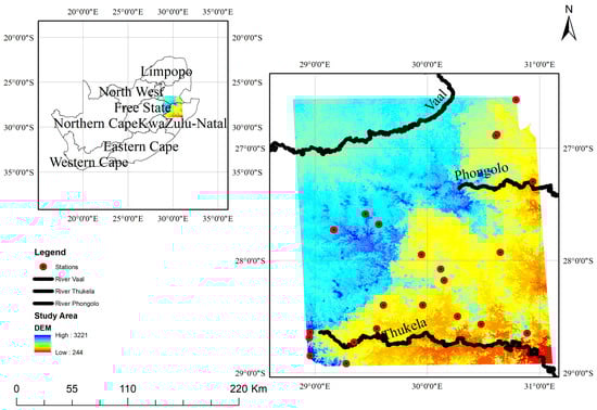
Figure 1.
The distribution of weather stations in the Enkangala Escarpment, shown over an elevation map of the study area.
2.2. Data and Analysis Procedures
Multi-decadal (1972–2022) variability and trends were examined for the Enkangala Escarpment using the trend-free pre-whitening Mann–Kendall (TFPWMK) test, innovative trend analysis (ITA), and Sen’s slope estimator [22,23,24,25].
Data analyses and mapping were carried out using R 4.0.2 using various packages such as moments for skewness calculation, TFPWMK, and ITA. ArcGIS 13.3 was used for spatial analysis. The spatial patterns of rainfall indices shown in the maps below were generated using inverse distance weighting (IDW) interpolation.
2.2.1. Rainfall Data
Monthly rainfall data for the area of interest were obtained from the South African Weather Service (SAWS) for the period between 1972 and 2023. Twenty-two stations located in the study area were selected based on the quality of their data. The missing value density across the station data ranges between 0.8 and 7.5%. The annual rainfall is defined from July to June of the following year, thereby encompassing the full summer rainfall season. The monthly data were used to determine the inter-annual variability in monthly, seasonal, and annual rainfall, as well as for the calculation of trends, over the period from 1972 to 2023. The seasons are defined as December to February (DJF summer), March to May (MAM autumn), June to August (JJA winter), and September to November (SON spring). While several studies have documented climate change trends for the eastern escarpment, often with a focus on the Maloti Drakensberg [4,13,16,17], this is the first study to explore trends for the Enkangala Escarpment in detail.
2.2.2. Missing Data Treatment
There is a low percentage of missing data in the 22 stations selected for this study because stations with more than 10% of missing data were rejected. The actual range of missing values per station is between 0.98 and 7.52% of the total record (Table 1). Missing rainfall data values were replaced using the simple Normal Ratio Method (NRM), which considers the influence of adjacent stations and their rainfall values, weighted by the normal annual rainfall [26,27]. It examines the correlation coefficients between the target station and nearby stations and uses the highest correlation coefficient for the infilling of the dataset.
v0 is the estimate of the missing value, Wi is the weight of the ith neighbouring station, and Vi is the value of the same variable at the ith station.
The weights of the neighbouring stations are calculated using Equation (2):
Wi is the weight of the ith station, ri is the correlation coefficient between the target station and the ith neighbouring station, and ni is the number of points used to calculate the correlation coefficient. This method is best suited if the annual rainfall at surrounding stations does not exceed 10% of the station requiring the replacement of missing values [28]. Stations within a 30 km radius are given priority for the replacement of missing data.

Table 1.
List of the stations and their characteristics (codes, latitude, longitude, altitude, and percentage of missing data).
Table 1.
List of the stations and their characteristics (codes, latitude, longitude, altitude, and percentage of missing data).
| No | Stations | Station Code | Lat | Lon | Alt (m) | % of Missing Data |
|---|---|---|---|---|---|---|
| 1 | Athole | F1 | −28.57 | 30.48 | 1557 | 6.0 |
| 2 | Bergville | F2 | −28.73 | 29.35 | 1145 | 4.4 |
| 3 | Blaauwkop | F3 | −28.5 | 30.27 | 1676 | 6.2 |
| 4 | Cavern | F4 | −28.64 | 28.96 | 1490 | 0.32 |
| 5 | Chelmsford | F5 | −27.95 | 29.95 | 1219 | 7.3 |
| 6 | Elandslaagte | F6 | −28.4 | 29.96 | 1050 | 6.3 |
| 7 | Glencoe | F7 | −28.18 | 30.15 | 1311 | 0 |
| 8 | Hattingspruit | F8 | −28.08 | 30.12 | 1310 | 2.7 |
| 9 | Memel | F9 | −27.68 | 29.57 | 1728 | 3.5 |
| 10 | Moorside | F10 | −28.4 | 29.61 | 1219 | 0.0 |
| 11 | Ncome | F11 | −27.93 | 30.65 | 1295 | 6.3 |
| 12 | Nerston | F12 | −26.57 | 30.79 | 1525 | 1.1 |
| 13 | Qudeni | F13 | −28.65 | 30.89 | 1524 | 6.3 |
| 14 | Rocco | F14 | −27.73 | 29.17 | 1844 | 2.2 |
| 15 | Roseleigh | F15 | −28.61 | 29.55 | 1145 | 1.1 |
| 16 | Royal Nat. Park | F16 | −28.69 | 28.95 | 1392 | 0.0 |
| 17 | Tafelkoppies | F17 | −26.88 | 30.62 | 1372 | 7.5 |
| 18 | Tygerfontein | F18 | −27.59 | 29.45 | 1852 | 0.2 |
| 19 | Verkykerskop | F19 | −28.92 | 29.28 | 1830 | 6.3 |
| 20 | Warden SK | F20 | −28.85 | 28.96 | 1052 | 2.2 |
| 21 | Waterval | F21 | −26.89 | 30.61 | 1190 | 6.3 |
| 22 | Zaaiplaat | F22 | −27.3 | 30.94 | 1631 | 5.1 |
2.3. Outlier Detection
Outlier detection and treatment is an important step because extreme values, whether low or high, can influence statistical analysis. Grubb’s test [29,30] is used to identify outliers. The dataset is assumed to be normally distributed except for the maximum value. Henceforth, using a defined significance level and number of observations affects the critical values for Grubbs’ test [29,30]. In this study, a p-value at a 0.05 significance level was used. The detected outliers are observations with Grubb’s test statistics greater than the calculated critical value of the dataset and with p-values less than 0.05. Monthly rainfall data from the 22 meteorological stations operated by SAWS over the period from 1972 to 2022 were subjected to Grubb’s test to detect outliers.
2.4. Rainfall Variability
Coefficient of Variation (CV)
The coefficient of variation (CV) is a positive definite statistic that quantifies how much the data points deviate from the average value [31]. Larger CV values indicate a higher variability around the mean value. Annual and seasonal rainfall variations for 22 rainfall stations in the Enkangala Escarpment from 1972 to 2023 were computed using CV, which was calculated as follows (in percent):
where σ is the standard deviation and μ denotes the average rainfall.
2.5. Trend Analysis
2.5.1. Mann–Kendall’s Trend Test
The Mann–Kendall non-parametric test is a robust test used for the trend analysis of climatic variables such as temperature and rainfall, as well as in hydrological studies such as the discharge of rivers and runoff analyses [32]. The MK test has been widely used in various applications because it is insensitive to the presence of outliers in the data [33,34,35]. A positive trend is indicated by positive values of the MK trend test’s results over time, while a negative trend is characterized by negative values [36].
The MK test is also widely used in trend analysis because it does not require the underlying dataset to be normally distributed, though its result may be affected by autocorrelation in the data.
Statistic S is computed as follows, where n is the sample length, xi are the individual precipitation values (i = 1, 2, …, –n − 1), and xj are the subsequent precipitation values (j = i + 1, i + 2, …, n) in the same series, as shown in Equations (4) and (5):
where
For series with more than 10 (n > 10) elements, the average distribution statistic is approximately equal to 0 with a variance determined by Equation (6) [37,38,39]. In most cases, the MK test is suitable for datasets containing more than 10 elements.
The number of records in the tied group is denoted with T(i), and m is the number of groups of the tied ranks. The standardized test statistic Z is computed.
Z is the MK test statistic, which is calculated with values of S and Var(S) using Equation (7)
The derived score Z is used to test the statistical significance of the trend. It is a two-tailed test: if |Z| ≥ Z (1 − α/2), the null hypothesis is rejected, while α is the significance level for the test. Positive values of Z show an increasing trend, and negative values denote a decreasing trend for the parameter. In this study, the two-tailed MK trend test was used to identify annual and seasonal rainfall trends for the Enkangala Escarpment of South Africa with a 95% confidence level.
2.5.2. Trend-Free Pre-Whitening Mann–Kendall (TFPWMK)
Each rain gauge time series is presumed to be serially independent in the sense that values at a particular time are not dependent on the values at any other time. However, the results of the MK test are frequently impacted by serial correlation in the hydro-meteorological time series [40,41]. For instance, the significance of the MK test is understated when there is a positive (negative) serial correlation in a time series [42,43,44]. Several pre-whitening approaches, including trend-free pre-whitening, have been designed to reduce the effects of serial correlation on the MK test findings, including the trend-free pre-whitening MK test (TFPWMK). This latter tool has been used because it has been shown that the MK test is less affected by serial correlation within the hydro-meteorological time series when first applying the pre-whitening step [45].
The initial step in TFPWMK involves normalizing the time series data by dividing each data point by the mean, removing any trends, and calculating the slope of the trend using Sen’s method. After identifying and addressing any lag-1 autocorrelation, the modified individual values are then reinserted into the original time series. Subsequently, the pre-whitened time series is analysed using the MK test.
2.5.3. Sen’s Slope Estimator
Sen’s slope estimator is a non-parametric method used to estimate the real slope of time series data [46]. The equation was used to calculate the median slope (Ti) of every data point.
The median of the slope values is between xj and xi of t at time steps j, where (i < j). A positive value signifies a positive trend, while a negative value signifies a negative trend. The sign conveys the positive or negative tendency of the data trend, while its magnitude reflects the trend’s steepness. This method has the benefit of reducing the impact of missing values or outliers on the slope, compared to the linear regression technique. While the MK test indicates whether a statistically significant trend exists in the data series, Sen’s slope estimator determines the magnitude of the trend [47].
2.5.4. Innovative Trend Analysis
The innovative trend analysis (ITA), first proposed in [48], can be used on homogenous variables irrespective of missing data and in the presence of the autocorrelation of the time series. The ITA test is not dependent on the length of the series, normality, and the serial correlation of the time series. It has been used as an alternative to the MK test and other forms of MK tests, which are supposed to solve the autocorrelation in the time series during the determination of the monotonic trend. Below is the detailed step-by-step procedure of ITA.
- The data (seasonal and annual) rainfall series is divided into two equal sub-series obtained from the original rainfall time series to conduct ITA.
- The obtained sub-series are arranged in increasing order.
- The first half of the sub-series rainfall time series is used on the x-axis (1972–1997), while the second half of the sub-series is used on the y-axis (1998–1922). It is plotted as a scatter plot.
- A straight line at 45° is drawn diagonally in the scatter plot coordinates, creating a 1:1 relationship and dividing the plot into upper and lower half triangles.
- If the scatter points fit perfectly on the 45° line, it indicates the lack of a trend; below the line indicates a negative trend, and above the line indicates an increasing trend.
- When all the scattered points are below or above upper or lower triangles, a series is considered to have a monotonic trend. It is a non-monotonic trend when some scattered points are in the upper half triangle and others in the lower half triangle.
The ITA test can also identify obscure trends, which is impossible with traditional methods because such methods can detect only monotonic trends [48,49].
The monthly ITA slope (s) can be calculated as follows [50]:
where x2 is the mean of the second half time series in ascending order, x1 is the mean of first half time series in ascending order, and n is the data length of the original time series. The slope is said to be significant at a given level of significance if it is less than the lower confidence limit or greater than the upper confidence limit. A 5% level was used to determine the significance of the slope.
3. Results and Discussion
3.1. Outlier
The application of Grubb’s test shows that at least one outlier was found for each of the stations, except at the Dundee and Warden SK stations, where no outliers were found. Outliers were detected for the months of January (14), February (3), November (1), and December (5) across the 22 stations.
3.2. Monthly, Seasonal, and Annual Rainfall Across the Enkangala Escarpment
The long-term average (1972–2022) monthly rainfall totals, averaged across the 22 stations located along the Enkangala Escarpment, are shown in Figure 2. The lowest month of rainfall is July, with an average of 7.48 mm of rainfall, while the month of January has the highest average monthly rainfall of 143.39 mm. Clearly, the Enkangala Escarpment displays pronounced dry–wet seasonality. The bulk of the rainfall occurs during the summer half-year, from October to March. The onset of the rainy season is in September, and its cessation is in April. During the dry season, soil moisture and vegetation dries out, resulting in high fire danger across the escarpment, peaking in September and October, until the onset of rainfall occurs [51].
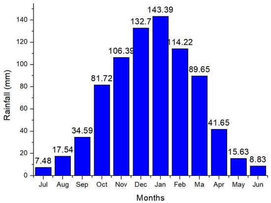
Figure 2.
The long-term average monthly rainfall across the 22 stations in Enkangala Escarpment for the period of 1972–2022.
The annual rainfall statistics for the Enkangala Escarpment for the period 1972 to 2022 are presented in Table 2. The meteorological station with the lowest recorded rainfall over a single calendar year over the 51-year period is Hattingspruit (254.5 mm), while the station that recorded the highest individual calendar year of rainfall is Royal National Park (RNP) (1916.9 mm). The annual median rainfall ranges between 639 mm and 1333.8 mm, with Memel and Qudeni being the stations with the lowest and highest values, respectively. The range of the mean annual rainfall is between 591.9 and 1343 mm, which demonstrates how vastly the rainfall totals vary across this area with its steep topographic slopes. The standard deviation (STD) of annual values varies from 136.3 to 305.9 mm (Warden SK and Royal National Park, respectively) for the period between 1972 and 2022, while the CV ranges from 18% to 28.05% (Elandslaagte and Hattingspruit, respectively).
Table 2.
The annual rainfall descriptive statistics from 1972 to 2022 over the Enkangala Escarpment.
Most of the rainfall distributions across the various stations are positively skewed except for seven stations, namely, Dannhauser, Dundee, Hattingspruit, Royal National Park, Volksrust, Waterval, and Warden SK. The range of the skewness is from −0.59 to 0.99, as recorded at Dannhauser and Zaaiplaats, respectively (Table 2). The kurtosis of the rainfall distribution patterns is positive at all stations and ranges from 2.27 to 4.98 at the Verkykerskop and Zaaiplaats stations, respectively.
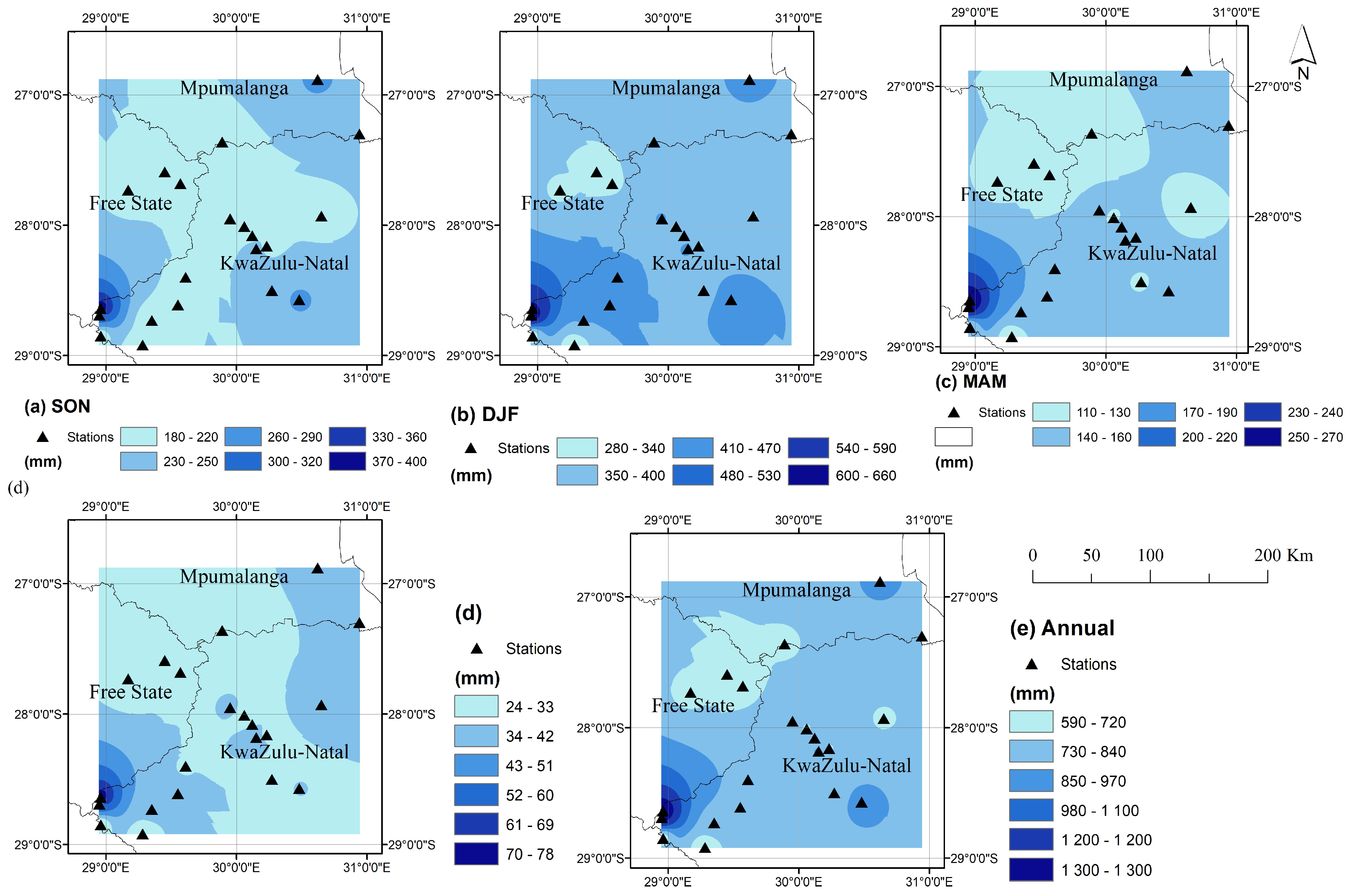
The spatial distribution of seasonal and annual rainfall over the study period is presented in Figure 3a–e. The onset of rainfall occurs in September, with SON totals peaking over the eastern domain and with a clear west–east gradient in rainfall (Figure 3a). Rainfall totals range between 180 and 220 mm in the west during spring, but with higher totals in the east and southwest. During DJF, general summer rainfall occurs over the Enkangala Escarpment, and the spatial distribution is more uniform compared to other seasons (Figure 3b). Most stations report between 350 and 400 mm of rain, with only the southern parts and far northeastern part of the domain receiving higher average summer rainfall. For MAM, rainfall varies between 110 and 160 mm over most of the domain, less than half of the DJF totals (Figure 3c). The effects of the escarpment can be clearly seen, with rainfall totals being higher east of the escarpment than over the plateau to the west. MAM rainfall peaks in the southwest, along the escarpment. JJA is the dry season, with most of the Enkangala Escarpment receiving less than 45 mm of rain during these months (Figure 3d). It is only along the escarpment in the southwest where higher totals are recorded in winter.

Figure 3.
(a–e) Mean seasonal rainfall from 1972 to 2022 across the Enkangala Escarpment, South Africa, for SON (a), DJF (b), MAM (c) JJA (d), and annual (e).
The annual rainfall spatial map is presented in Figure 3e. Generally, rainfall totals are higher to the southeast of the escarpment compared to over the plateau. Mean annual rainfall varies between a minimum of 593 mm at Verkykerskop in the western and central part of the escarpment to a maximum of 1343 mm at Cavern Farm, located close to Lesotho. Based on the 22 stations of rainfall data analysed, approximately 65% of the escarpment, on average, receives rainfall between 720 mm and 820 mm per annum. Less than 5% of the region receives more than 1000 mm annually, and less than 15% receives rainfall between 600 mm and 720 mm per annum.
3.3. Rainfall Variability 1972–2022
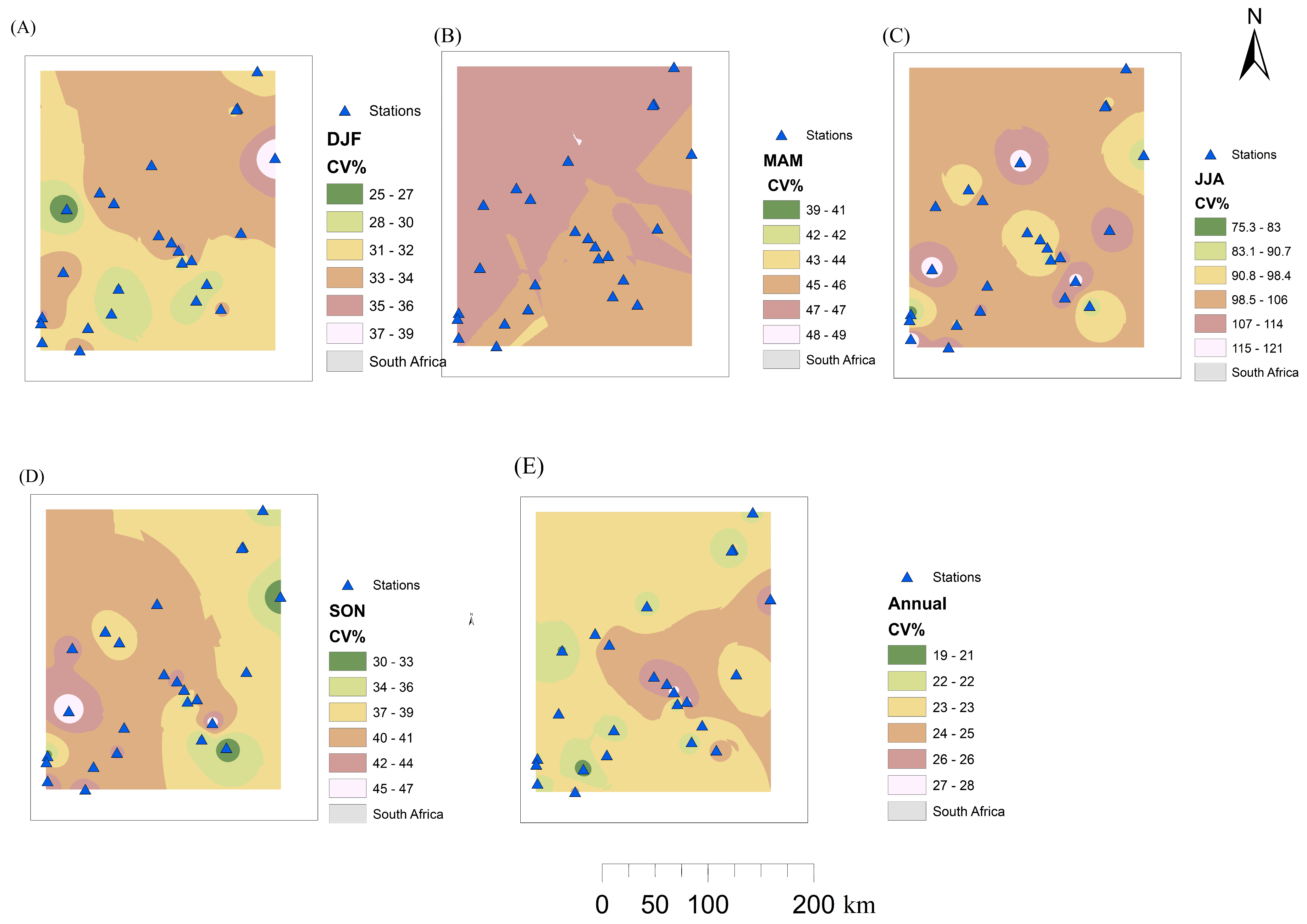
The spatial distribution of rainfall variability over Enkangala Escarpment is presented in Figure 4. The CV values are expressed in percentages. The JJA season is the most variable, with CV values between 80.3% and 149% as recorded at the Qudeni and Cavern Farm stations, respectively (Figure 4C). The range of CV values during the SON season is between 30 and 49%, as recorded in Athole and Elandslaagte (Figure 4D). The Glencoe and Cavern Farm stations recorded the minimum and highest CV values for the MAM season, with values of 39 and 49%, respectively (Figure 4B). For DJF, CV values range between 25 and 39% across the stations, with the Rocco and Zaaiplaat stations having recorded the minimum and maximum CV values, respectively (Figure 4A). This substantial variability in summer rainfall over the Enkangala Escarpment is well known to be strongly influenced by ENSO (7). This pronounced inter-annual variability in rainfall has implications for agriculture, as well as for the dams (Ingula dam and Drakensberg Dam), which are critical for power generation irrigation and municipal water supply. The annual variability is lower than the seasonal variability. The annual coefficients of variation (CV) calculated for the rainfall dataset for the period from 1972 to 2022 ranged between 19% and 39%, found at the Glencoe and Warden SK stations (Figure 4E).
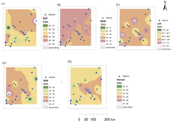
Figure 4.
The spatial distribution of the coefficient of variation (CV%) over the Enkangala Escarpment for the period of 1972–2022. Seasonal: DJF (A), MAM (B), JJA (C), SON (D), and annual (E).
3.4. Rainfall Trend Analysis
This section discusses the annual and seasonal rainfall trends for the 22 stations in the Enkangala Escarpment. The TFPWMK test was applied at the 95% confidence level, p = 0.05, to produce the Mann–Kendall trend statistic, Z. The ITA method was used to produce the slope values and slope standard deviation, and related confidence intervals.
3.4.1. Trends in Annual Rainfall
The TFPWMK tests detected a significantly decreasing (negative) rainfall trend at seven stations, twelve non-significant decreasing trends, one station (Tafelkoppies) with a significant increasing trend, and two stations (Chelmsford and Rocco) with non-significant increasing trends (Table 3). On the other hand, the ITA method detected seventeen stations with significantly decreasing trends, one station (Bergville) with a non-significant decreasing trend, one with a significant increasing trend (Cavern Farm), and three stations (Chelmsford, Rocco, and Tafelkoppies) with non-significant increasing trends (Table 3 and Figure 5).
Table 3.
Trends in annual and seasonal rainfall over the Enkangala Escarpment. A single asterisk indicates statistical significance at the 5% level while ‘−’ and ‘+’ indicate negative and positive trends, respectively.
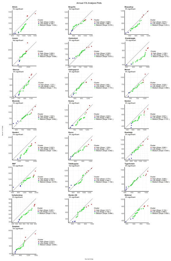
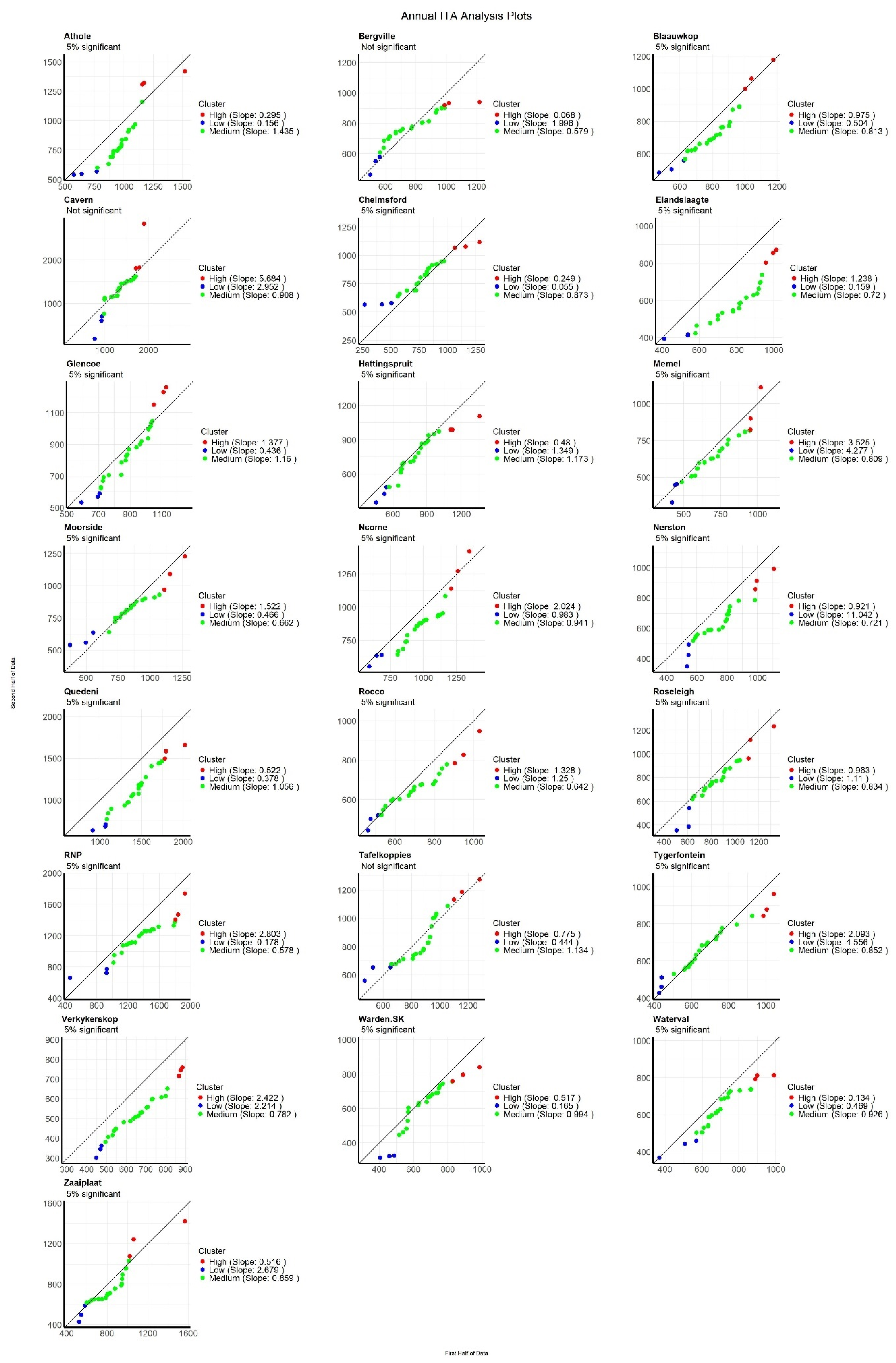
Figure 5.
The annual ITA test results for different stations of the Enkangala Escarpment. The orange, blue, and green points represent the intervals of the high, low, and medium rainfall, respectively.
The black lines in Figure 5 represent the trends of the original time series, while the remaining colours represent sub-trends. In the high cluster, Caven station experienced the highest decreasing trend (5.68 mm/decade). On the other hand, the Bergville station experienced the lowest decreasing trend (0.07 mm/decade). In the medium cluster, the Athole station experienced the highest decreasing trend (1.44 mm/decade), and the lowest was the RNP station (0.58 mm/decade). Nerston (11.04 mm/decade) and Chelmsford (0.06 mm/decade) are the stations with the highest and lowest decreasing trends in the low cluster (Figure 5).
The magnitudes of Sen’s slope indicating decreases in annual rainfall across the Enkangala Escarpment was as large as 7.46 mm/decade (at Elandslaagte, Table 4). The slopes of the ITA method indicate negative trends as large as 7.96 mm/decade (Table 4; Tygerfontein).
Table 4.
The magnitude of annual rainfall trends obtained from the TFPWMK and ITA trends and methods of analysis (note that RNP stands for Royal National Park, CI: confidence interval, SSD: slope standard deviation, Y: Yes and N: No).
3.4.2. Trends in SON Rainfall
For the SON season, the TFPWMK test detected 13 stations with significantly decreasing trends and nine stations with non-significantly decreasing trends. There were zero stations with increasing trends (Table 5 and Table 6). The ITA method detected 21 stations with significantly decreasing trends and only one station (Chelmsford) with a non-significant decreasing trend. The rest of the stations did not experience either significant increasing trends or non-significant increasing trends at 5% significance levels.
Table 5.
The magnitude of SON seasonal rainfall trends obtained from the TFPWMK and ITA trends and methods of analysis. The units of the slopes are for the rate of change in SON rainfall in mm/decade (note that RNP stands for Royal National Park, CI: confidence interval, SSD: slope standard deviation, Y: Yes and N: No).
Table 6.
The magnitude of the DJF seasonal rainfall trends obtained from the TFPWMK and ITA trends and methods of analyses (note that, RNP stands for Royal National Park, CI: confidence interval, SSD: slope standard deviation, Y: Yes and N: No).
The SON seasonal rainfall magnitudes of Sen’s slope significantly decreased at ranges between 1.29 and 4.85 mm/decade (Table 5). The slopes of the ITA method indicate that the Tafelkoppies station experienced the least decreasing trend, whereas Quedeni experienced the highest decreasing trend across the stations. The ITA slope ranges from −0.25 to −3.70 mm/decade (Table 5).
3.4.3. The DJF Seasonal Rainfall Trend Analysis
From the TFPWMK tests, only the Elandslaagte station experienced a significantly decreasing trend, with 14 stations showing non-significantly decreasing trends. None of the stations had a significantly increasing trend, with seven stations having non-significantly increasing trends in their DJF rainfall distribution over the study period at a 5% significance level (Table 3 and Table 6). The ITA method detected 21 stations with significantly decreasing trends, and only one station (Chelmsford) showed a non-significantly decreasing trend. The rest of the stations did not experience either significantly increasing trends or a non-significantly increasing trend at a 5% significance level.
The DJF seasonal rainfall magnitudes of Sen’s slope significantly decreased at values between 1.29 and 4.85 mm/decade (Table 7, Figure 6). The slopes of the ITA method indicate that the Tafelkoppies station experienced the least decreasing trend, whereas Quedeni experienced the highest decreasing trend across the stations. The ITA slope ranges from −0.25 to −3.70 mm/decade (Table 7).
Table 7.
The magnitude of the MAM seasonal rainfall trends obtained from the TFPWMK and ITA trends and methods of analyses (note that RNP stands for Royal National Park, CI: confidence interval, SSD: slope standard deviation, Y: Yes and N: No).
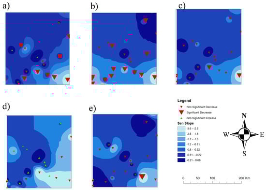
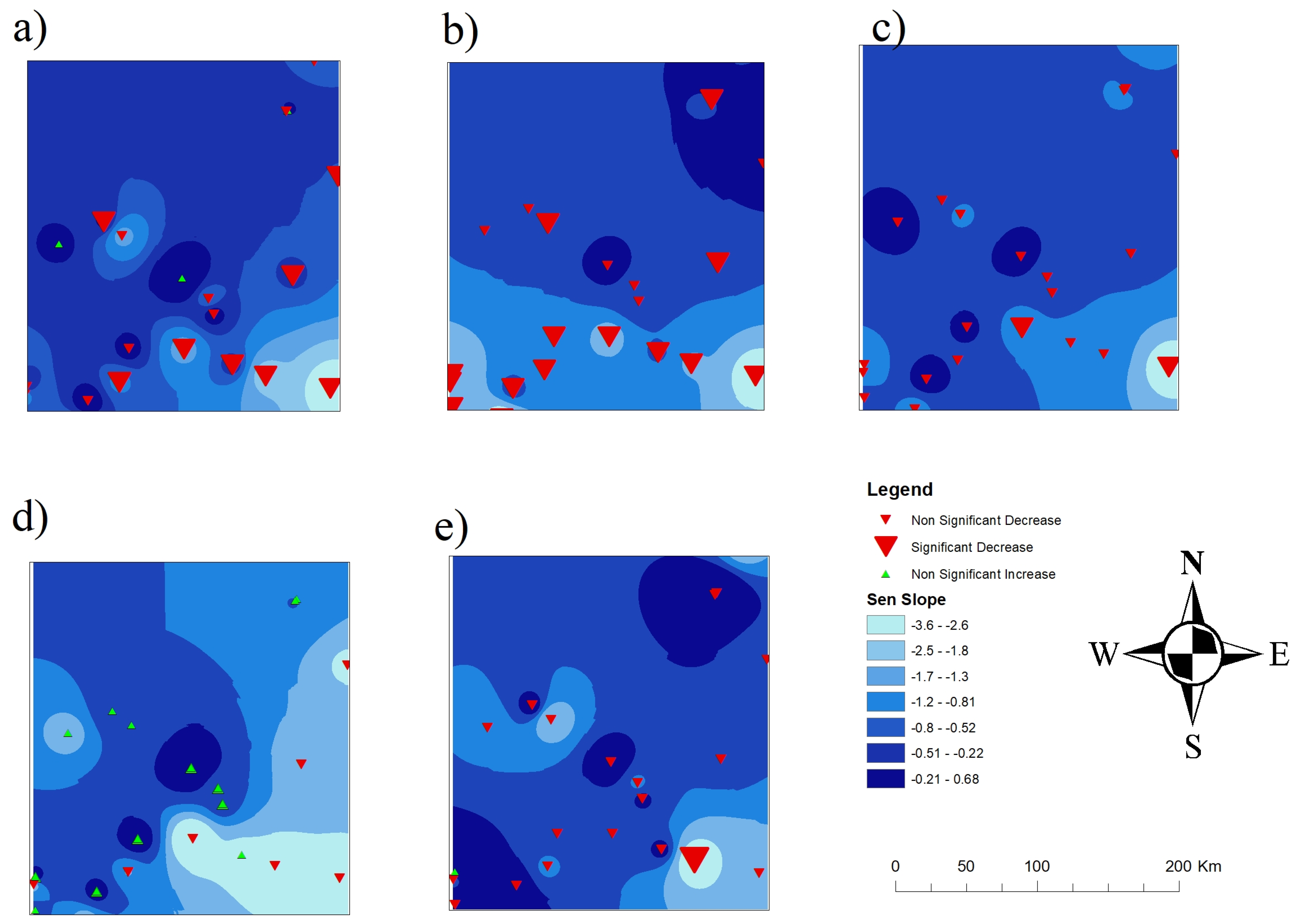
Figure 6.
The spatial distributions of the Sen slopes for the trend analyses over the Enkangala Escarpment for the period 1972–2022, (a): Annual, (b): SON, (c): DJF, (d): MAM, (e): JJA. NSD denotes non-significant decrease, SD denotes significant decrease, NSI denotes non-significant increase, and SI denotes significant increase.
3.4.4. The MAM Seasonal Rainfall Trend Analysis
Using the TFPWMK tests, there is not a single station with a significantly decreasing trend during the MAM season. Seven stations experienced non-significantly decreasing trends at a 5% confidence level. Likewise, there are zero stations with a significant increasing trend; however, 15 stations experienced a non-significantly increasing trend in MAM at a 5% significance level (Table 3 and Table 7). The ITA method detected seven stations with significantly decreasing trends (Athole Elandslaagte, Quedeni, Ncome, Verkykerskop, and Zaaiplaat) and two stations (Hattingspruit and RNP) with a non-significant decreasing trend. According to the ITA test, there are 12 stations that have experienced significantly increasing trends and two stations (Memel and RNP) with a non-significantly increasing trend at a 5% significance level. The MAM seasonal rainfall magnitudes of Sen’s slope were insignificantly decreasing at ranges between 0.27 and 0.76 mm/decade (Table 8. The slopes of the ITA method indicate that Hattingspruit station experienced the least decreasing trend, whereas Athole experienced the highest decreasing trend across the stations. The ITA slope ranges from −0.05 to −0.88 mm/decade, with four stations reporting increasing trends between 0.14 and 1.16 mm/decade (Table 7).
Table 8.
The magnitude of the JJA seasonal rainfall trends obtained from the TFPWMK and ITA trends and methods of analysis (note that, RNP stands for Royal National Park, CI: confidence interval, SSD: slope standard deviation, Y: Yes and N: No).
3.4.5. The JJA Seasonal Rainfall Trend Analysis
According to the TFPWMK tests, the Athole station is the only station with a significantly decreasing trend during the JJA season. Twenty stations experienced non-significantly decreasing trends at a 5% confidence level. Also, there were zero stations with significant trends; however, one station (Cavern) experienced a non-significant increasing trend (Table 3 and Table 8). The ITA method detected 17 stations with significantly decreasing trends, with two stations (Hattingspruit and Tafelkoppies) experiencing a non-significant decreasing trend. Bergville is the only station that experienced a non-significantly increasing trend. Cavern Farm station and Waterval are the only stations with significantly increasing trends during the JJA season.
The JJA seasonal rainfall magnitudes of Sen’s slope showed an insignificantly decreasing trend at ranges between 0.16 and 0.62 mm/decade (Table 8). The slopes of the ITA method indicate that the Blaauwkop station experienced the least decreasing trend, whereas Nerston experienced the highest decreasing trend across the stations. The ITA slope ranges between –0.08 and –0.59 mm/decade; meanwhile, the Waterval and Cavern stations experienced increasing trends of between 0.16 and 1.42 mm/decade (Table 8).
3.5. Spatial Trend Analyses
Figure 6 shows the results of Sen’s slope regarding annual and seasonal rainfall. This figure clearly indicates stations with increasing and decreasing trends graphically, with the spatial interpolation of Sen’s slope produced using the ordinary Kriging method. The Sen slopes were determined at significance (p < 0.05). Statistically significant decreases in annual rainfall can be detected over the southern and eastern escarpment areas, with mostly non-significant decreasing trends elsewhere.
SON is the season that exhibits spatially homogeneous and negative rainfall trends across the entire Enkangala Escarpment, with the trends being statistically significant in the southern and eastern parts. The DJF trends are similarly indicative of a decline in rainfall across the area of interest but are mostly without local statistical significance. The MAM trends are spatially heterogeneous and mostly without local statistical significance, while the JJA trends are mostly negative but generally without local statistical significance.
3.6. Comparative Analysis of the TFPWMK with ITA Test
Out of the 22 weather stations’ annual trends, 7 stations (31.8%) exhibited significantly decreasing trends using the TFPWMK method, while 17 stations (72.3%) showed significantly decreasing trends using the ITA method (Figure 7e). The stations with significantly decreasing trends according to the ITA methodinclude the seven stations detected using the TFPWMK method. Both methods detected one station (Tafelkoppies) with a significantly increasing trend.
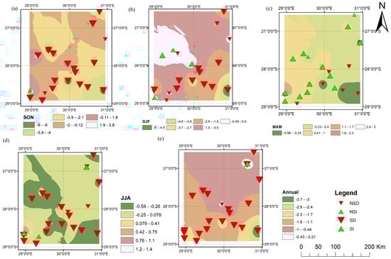
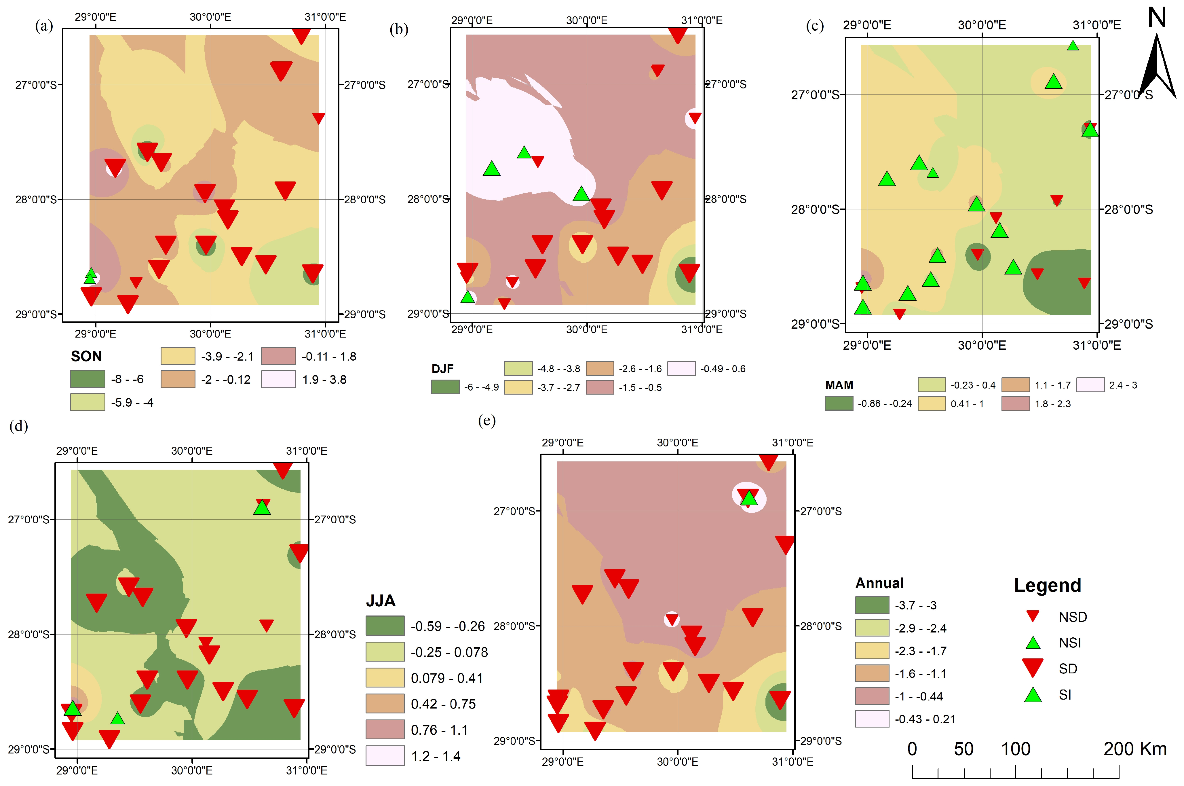
Figure 7.
The spatial distributions of the ITA trend analysis over the Enkangala Escarpment for the period 1972–2022, (a): Annual, (b): SON, (c): DJF, (d): MAM, (e): JJA. NSD denotes non-significant decrease, SD denotes significant decrease, NSI denotes non-significant increase, and SI denotes significant increase.
For SON, the TFPWMK method detected 14 stations (63.5%) and the ITA method 21 stations (95.5%) with significant decreasing trends in spring rainfall (Figure 7a). For DJF, only one station was detected with a significant decreasing trend using the TFPWMK method; however, the ITA method detected 12 stations (55%) with significant decreasing trends (Figure 7b).
For the MAM season, the TFPWMK test detected zero stations with any form of significant trend; however, the ITA test captured 7 stations and 12 stations with statistically decreasing and increasing trends, respectively (Figure 7c). Finally, the JJA seasonal trends described by the TFWMK test showed only one station (9.01%) with a significant decreasing trend, while 17 (77.27%) stations exhibit a significantly decreasing trend according to the ITA method (Figure 7d). These results suggest that the ITA test is more sensitive in terms of detecting significant trends. The results are similar to previous studies which showcase the sensitivity of ITA over other trend analysis methods [52,53]. Kavwenje et al. (2024) [54] used ITA to detect seasonal and annual trends in rainfall over Malawi and compared the results obtained from Mann–Kendall (MK) and Spearman rho (SMR) tests with statistical-graphical methods of the Onyutha trend (OT) test. ITA is more sensitive in detecting hidden trends not detected by conventional, nonparametric, and graphical trend methods.
4. Conclusions
This study presents annual and seasonal rainfall trends as well as an analysis of inter-annual variability in rainfall for 22 rainfall stations located on the Enkangala Escarpment of South Africa, over the period 1972–2022 (51 years). The CV analyses quantify the well-known inter-annual variability in seasonal rainfall over the Enkangala Escarpment; it is against the background of this natural variability that systematic rainfall trends may occur.
The TFPWMK and ITA trend tests were used to detect the trends. The TFPWMK test seems to be less sensitive in the detection of significant local trends. The ITA method has detected more statistically significant trends across the different seasons, consistent with other research [50,54]. Both the TFPWMK and ITA tests are indicative of a spatial coherency in negative winter, spring, and summer rainfall trends across the Enkangala Escarpment. For winter and summer, the negative trends are mostly without local statistical significance; however, their spatial coherency is nevertheless indicative of a systematic change in rainfall across the region. For spring, the negative trends are mostly also locally statistically significant. The autumn trends are spatially heterogeneous and, in general, without local statistical significance. The negative trends in winter rainfall are of little physical significance, given that winter rainfall totals in this region are very low to begin with. However, the substantial reductions in spring rainfall are highly significant since this implies less favorable conditions during the early growing season of crops in terms of soil moisture availability. Projected decreases in spring rainfall also translate into later onset dates (for planting) and a longer burning season. The decreases can probably be attributed to increased subsidence occurring over southern Africa in a warming world, in response to the more frequent and intense mid-level, high-pressure systems over southern Africa in winter and spring. This change in the regional circulation in response to anthropogenic forcing was first projected to occur by (Engelbrecht et al., 2009) [55] links to the intensification of the regional Hadley Cell circulation. The spatial coherency of negative summer rainfall trends, although generally without local significance, is nevertheless concerning, should this trend amplify deeper into the 21st century under ongoing global warming.
Author Contributions
H.B.A.: Conceptualization, Data acquisition, Formal analysis, Investigation, Methodology, Visualization, Writing—original draft; M.C.S.: Conceptualization, Resources; F.A.E.: Review and editing. All authors have read and agreed to the published version of the manuscript.
Funding
This work was supported by Forestry South Africa (SA Forestry), grant number FSA2020 and the National Research Foundation project, LongDrySpell, Grant ID 136480.
Institutional Review Board Statement
Not applicable.
Informed Consent Statement
Not applicable.
Data Availability Statement
The data were obtained from the South Africa weather service.
Acknowledgments
The authors are grateful to the South Africa Weather Services (SAWS) for providing datasets for the research. We also acknowledge the support from Forestry South Africa (FSA) for funding (FSA2020).
Conflicts of Interest
The author declares that there are no conflicts of interest.
References
- Engelbrecht, F.A.; Marean, C.W.; Cowling, R.M.; Engelbrecht, C.J.; Neumann, F.H.; Scott, L.; Nkoana, R.; O’Neal, D.; Fisher, E.; Shook, E. Downscaling last glacial maximum climate over southern Africa. Quat. Sci. Rev. 2019, 226, 105879. [Google Scholar] [CrossRef]
- Mills, S.C.; Grab, S.W.; Rea, B.R.; Carr, S.J.; Farrow, A. Shifting westerlies and precipitation patterns during the Late Pleistocene in southern Africa determined using glacier reconstruction and mass balance modelling. Quat. Sci. Rev. 2012, 55, 145–159. [Google Scholar] [CrossRef]
- Taylor, S.; Ferguson, J.; Engelbrecht, F.A.; Clark, V.; Van Rensburg, S.; Barker, N. The Drakensberg Escarpment as the great supplier of water to South Africa. In Developments in Earth Surface Processes; Elsevier: Amsterdam, The Netherlands, 2016; Volume 21, pp. 1–46. [Google Scholar]
- Engelbrecht, F.A.; Monteiro, P. The IPCC assessment report six working group 1 report and southern Africa: Reasons to take action. S. Afr. J. Sci. 2021, 117, 1–7. [Google Scholar] [CrossRef] [PubMed]
- Engelbrecht, F.A.; Steinkopf, J.; Padavatan, J.; Midgley, G.F. Projections of future climate change in southern Africa and the potential for regional tipping points. In Sustainability of Southern African Ecosystems Under Global Change: Science for Management and Policy Interventions; Springer: Berlin/Heidelberg, Germany, 2024; pp. 169–190. [Google Scholar]
- Ndlovu, E.; Prinsloo, B.; Le Roux, T. Impact of climate change and variability on traditional farming systems: Farmers’ perceptions from south-west, semi-arid Zimbabwe. Jàmbá J. Disaster Risk Stud. 2020, 12, 1–19. [Google Scholar] [CrossRef]
- Steinkopf, J.; Engelbrecht, F. Verification of ERA5 and ERA-Interim precipitation over Africa at intra-annual and interannual timescales. Atmos. Res. 2022, 280, 106427. [Google Scholar] [CrossRef]
- Ibebuchi, C.C. Circulation patterns linked to the positive sub-tropical Indian ocean dipole. Adv. Atmos. Sci. 2023, 40, 110–128. [Google Scholar] [CrossRef]
- Hart, N.C.; Reason, C.J.; Fauchereau, N. Cloud bands over southern Africa: Seasonality, contribution to rainfall variability and modulation by the MJO. Clim. Dyn. 2013, 41, 1199–1212. [Google Scholar] [CrossRef]
- Ndarana, T.; Mpati, S.; Bopape, M.-J.M.; Engelbrecht, F.A.; Chikoore, H. The flow and moisture fluxes associated with ridging South Atlantic Ocean anticyclones during the subtropical southern African summer. Int. J. Climatol. 2021, 41, E1000–E1017. [Google Scholar] [CrossRef]
- Xulu, N.G.; Chikoore, H.; Bopape, M.-J.M.; Ndarana, T.; Muofhe, T.P.; Mbokodo, I.L.; Munyai, R.B.; Singo, M.V.; Mohomi, T.; Mbatha, S.M. Cut-off lows over South Africa: A review. Climate 2023, 11, 59. [Google Scholar] [CrossRef]
- Mbokodo, I.L.; Bopape, M.-J.M.; Ndarana, T.; Mbatha, S.M.; Muofhe, T.P.; Singo, M.V.; Xulu, N.G.; Mohomi, T.; Ayisi, K.K.; Chikoore, H. Heatwave variability and structure in South Africa during summer drought. Climate 2023, 11, 38. [Google Scholar] [CrossRef]
- Ncoyini, Z.; Savage, M.; Strydom, S. Limited access and use of climate information by small-scale sugarcane farmers in South Africa: A case study. Clim. Serv. 2022, 26, 100285. [Google Scholar] [CrossRef]
- Meza, I.; Rezaei, E.E.; Siebert, S.; Ghazaryan, G.; Nouri, H.; Dubovyk, O.; Gerdener, H.; Herbert, C.; Kusche, J.; Popat, E. Drought risk for agricultural systems in South Africa: Drivers, spatial patterns, and implications for drought risk management. Sci. Total Environ. 2021, 799, 149505. [Google Scholar] [CrossRef] [PubMed]
- Bello, A.H.; Scholes, M.C.; Francois, E.A. Spatio-temporal trends in daily precipitation extremes over the Enkangala escarpment of South Africa: 1961–2021. Theor. Appl. Climatol. 2025, 156, 164. [Google Scholar]
- Alahacoon, N.; Edirisinghe, M.; Simwanda, M.; Perera, E.; Nyirenda, V.R.; Ranagalage, M. Rainfall Variability and Trends over the African Continent Using TAMSAT Data (1983–2020): Towards Climate Change Resilience and Adaptation. Remote Sens. 2021, 14, 96. [Google Scholar] [CrossRef]
- Scholes, R.; Engelbrecht, F. Climate Impacts in Southern Africa During the 21st Century; Report for Earthjustice and the Centre for Envrionmental Rights; Global Change Instiute, University of Witwatersrand: Johannesburg, South Africa, 2021. [Google Scholar]
- Becker, A.; Finger, P.; Meyer-Christoffer, A.; Rudolf, B.; Schamm, K.; Schneider, U.; Ziese, M. A description of the global land-surface precipitation data products of the Global Precipitation Climatology Centre with sample applications including centennial (trend) analysis from 1901–present. Earth Syst. Sci. Data 2013, 5, 71–99. [Google Scholar] [CrossRef]
- Zuma-Netshiukhwi, G.; Stigter, K.; Walker, S. Use of traditional weather/climate knowledge by farmers in the South-western Free State of South Africa: Agrometeorological learning by scientists. Atmosphere 2013, 4, 383–410. [Google Scholar] [CrossRef]
- Wilhite, D.A.; Sivakumar, M.V.; Pulwarty, R. Managing drought risk in a changing climate: The role of national drought policy. Weather Clim. Extrem. 2014, 3, 4–13. [Google Scholar] [CrossRef]
- Tall, A.; Hansen, J.; Jay, A.; Campbell, B.M.; Kinyangi, J.; Aggarwal, P.K.; Zougmoré, R.B. Scaling Up Climate Services for Farmers: Mission Possible. Learning from Good Practice in Africa and South Asia; CCAFS Report; CCAFS: Johannesburg, South Africa, 2014. [Google Scholar]
- van der Walt, A.J.; Fitchett, J.M. Exploring extreme warm temperature trends in South Africa: 1960–2016. Theor. Appl. Climatol. 2021, 143, 1341–1360. [Google Scholar] [CrossRef]
- Yue, S.; Wang, C.Y. Regional streamflow trend detection with consideration of both temporal and spatial correlation. Int. J. Climatol. A J. R. Meteorol. Soc. 2002, 22, 933–946. [Google Scholar] [CrossRef]
- Khan, F.; Ali, S.; Ullah, H.; Muhammad, S. Twenty-first century climate extremes’ projections and their spatio-temporal trend analysis over Pakistan. J. Hydrol. Reg. Stud. 2023, 45, 101295. [Google Scholar] [CrossRef]
- Baig, M.R.I.; Shahfahad; Naikoo, M.W.; Ansari, A.H.; Ahmad, S.; Rahman, A. Spatio-temporal analysis of precipitation pattern and trend using standardized precipitation index and Mann–Kendall test in coastal Andhra Pradesh. Model. Earth Syst. Environ. 2022, 8, 2733–2752. [Google Scholar]
- Te Chow, V. Applied Hydrology; Tata McGraw-Hill Education: New York, NY, USA, 2010. [Google Scholar]
- Linsley, R.K., Jr.; Kohler, M.A.; Paulhus, J.L. Hydrology for Engineers; McGraw-Hill College: New York, NY, USA, 1975. [Google Scholar]
- Tang, W.; Kassim, A.; Abubakar, S. Comparative studies of various missing data treatment methods-Malaysian experience. Atmos. Res. 1996, 42, 247–262. [Google Scholar] [CrossRef]
- Urvoy, M.; Autrusseau, F. Application of Grubbs’ test for outliers to the detection of watermarks. In Proceedings of the 2nd ACM Workshop on Information Hiding and Multimedia Security, Salzburg, Austria, 13 June 2014; pp. 49–60. [Google Scholar]
- Mallick, J.; Talukdar, S.; Alsubih, M.; Salam, R.; Ahmed, M.; Kahla, N.B.; Shamimuzzaman, M. Analysing the trend of rainfall in Asir region of Saudi Arabia using the family of Mann-Kendall tests, innovative trend analysis, and detrended fluctuation analysis. Theor. Appl. Climatol. 2021, 143, 823–841. [Google Scholar] [CrossRef]
- Pélabon, C.; Hilde, C.H.; Einum, S.; Gamelon, M. On the use of the coefficient of variation to quantify and compare trait variation. Evol. Lett. 2020, 4, 180–188. [Google Scholar]
- Anekwe, I.M.S.; Zhou, H.; Mkhize, M.M.; Akpasi, S.O. Effects of Climate Change on Agricultural Production in South Africa. Int. J. Clim. Change Impacts Responses 2023, 15. [Google Scholar]
- Wang, W.; Chen, X.; Shi, P.; Van Gelder, P.; Corzo, G. Extreme precipitation and extreme streamflow in the Dongjiang River Basin in southern China. Hydrol. Earth Syst. Sci. Discuss. 2007, 4, 2323–2360. [Google Scholar]
- Hamed, K.H. Trend detection in hydrologic data: The Mann–Kendall trend test under the scaling hypothesis. J. Hydrol. 2008, 349, 350–363. [Google Scholar]
- Ali, R.; Kuriqi, A.; Abubaker, S.; Kisi, O. Long-term trends and seasonality detection of the observed flow in Yangtze River using Mann-Kendall and Sen’s innovative trend method. Water 2019, 11, 1855. [Google Scholar] [CrossRef]
- Gadgil, A.; Dhorde, A. Temperature trends in twentieth century at Pune, India. Atmos. Environ. 2005, 39, 6550–6556. [Google Scholar]
- Roy, T.; Lepcha, K. Analysis of rainfall variability and trend in a small homogenous region of West Bengal in Malda district. Arab. J. Geosci. 2023, 16, 595. [Google Scholar]
- Nouaceur, Z.; Murărescu, O. Rainfall variability and trend analysis of annual rainfall in North Africa. Int. J. Atmos. Sci. 2016, 2016, 7230450. [Google Scholar] [CrossRef]
- Machiwal, D.; Gupta, A.; Jha, M.K.; Kamble, T. Analysis of trend in temperature and rainfall time series of an Indian arid region: Comparative evaluation of salient techniques. Theor. Appl. Climatol. 2019, 136, 301–320. [Google Scholar] [CrossRef]
- Almazroui, M.; Şen, Z. Trend analyses methodologies in hydro-meteorological records. Earth Syst. Environ. 2020, 4, 713–738. [Google Scholar] [CrossRef]
- Citakoglu, H.; Minarecioglu, N. Trend analysis and change point determination for hydro-meteorological and groundwater data of Kizilirmak basin. Theor. Appl. Climatol. 2021, 145, 1275–1292. [Google Scholar] [CrossRef]
- Jin, S.; Ma, Y.; Huang, Z.; Huang, J.; Gong, W.; Liu, B.; Wang, W.; Fan, R.; Li, H. A Comprehensive Reappraisal of Long-term Aerosol Characteristics, Trends, and Variability in Asia. Atmos. Chem. Phys. 2023, 23, 8187–8210. [Google Scholar] [CrossRef]
- Tan, X.; Wu, Y.; Liu, B.; Chen, S. Inconsistent changes in global precipitation seasonality in seven precipitation datasets. Clim. Dyn. 2020, 54, 3091–3108. [Google Scholar] [CrossRef]
- Adeyeri, O.; Laux, P.; Ishola, K.; Zhou, W.; Balogun, I.; Adeyewa, Z.; Kunstmann, H. Homogenising meteorological variables: Impact on trends and associated climate indices. J. Hydrol. 2022, 607, 127585. [Google Scholar] [CrossRef]
- Karki, R.; Hasson, S.u.; Schickhoff, U.; Scholten, T.; Böhner, J. Rising precipitation extremes across Nepal. Climate 2017, 5, 4. [Google Scholar] [CrossRef]
- Sen, P.K. Estimates of the regression coefficient based on Kendall’s tau. J. Am. Stat. Assoc. 1968, 63, 1379–1389. [Google Scholar] [CrossRef]
- Peterson, T.C.; Stott, P.A.; Herring, S. Explaining extreme events of 2011 from a climate perspective. Bull. Am. Meteorol. Soc. 2012, 93, 1041–1067. [Google Scholar] [CrossRef]
- Şen, Z. Innovative trend analysis methodology. J. Hydrol. Eng. 2012, 17, 1042–1046. [Google Scholar] [CrossRef]
- Chowdari, K.; Deb Barma, S.; Bhat, N.; Girisha, R.; Gouda, K.; Mahesha, A. Trends of seasonal and annual rainfall of semi-arid districts of Karnataka, India: Application of innovative trend analysis approach. Theor. Appl. Climatol. 2023, 152, 241–264. [Google Scholar]
- Şen, Z. Innovative trend significance test and applications. Theor. Appl. Climatol. 2017, 127, 939–947. [Google Scholar]
- Engelbrecht, F.; Adegoke, J.; Bopape, M.-J.; Naidoo, M.; Garland, R.; Thatcher, M.; McGregor, J.; Katzfey, J.; Werner, M.; Ichoku, C. Projections of rapidly rising surface temperatures over Africa under low mitigation. Environ. Res. Lett. 2015, 10, 085004. [Google Scholar] [CrossRef]
- Arab Amiri, M.; Gocić, M. Innovative trend analysis of annual precipitation in Serbia during 1946–2019. Environ. Earth Sci. 2021, 80, 777. [Google Scholar]
- Singh, R.; Sah, S.; Das, B.; Potekar, S.; Chaudhary, A.; Pathak, H. Innovative trend analysis of spatio-temporal variations of rainfall in India during 1901–2019. Theor. Appl. Climatol. 2021, 145, 821–838. [Google Scholar]
- Kavwenje, S.; Zhao, L.; Chen, L.; Ngongondo, C.; Chaima, E.; Aborisade, M.A.; Oba, B.T.; Kumambala, P. Integrated statistical and graphical non-parametric trenxd analysis of annual and seasonal rainfall in the Shire River Basin, Malawi. Theor. Appl. Climatol. 2024, 155, 2053–2069. [Google Scholar]
- Engelbrecht, F.A.; McGregor, J.L.; Engelbrecht, C.J. Dynamics of the conformal-cubic atmospheric model projected climate-change signal over southern Africa. Int. J. Climatol. 2009, 29, 1013–1033. [Google Scholar] [CrossRef]


Disclaimer/Publisher’s Note: The statements, opinions and data contained in all publications are solely those of the individual author(s) and contributor(s) and not of MDPI and/or the editor(s). MDPI and/or the editor(s) disclaim responsibility for any injury to people or property resulting from any ideas, methods, instructions or products referred to in the content. |
© 2025 by the authors. Licensee MDPI, Basel, Switzerland. This article is an open access article distributed under the terms and conditions of the Creative Commons Attribution (CC BY) license (https://creativecommons.org/licenses/by/4.0/).