Article

The Relationship Between Surface Meteorological Variables and Air Pollutants in Simulated Temperature Increase Scenarios in a Medium-Sized Industrial City

by
Ronan Adler Tavella
1,2,*,
Daniele Feijó das Neves
2,
Gustavo de Oliveira Silveira
3,
Gabriella Mello Gomes Vieira de Azevedo
3,
Rodrigo de Lima Brum
3,
Alicia da Silva Bonifácio
3,
Ricardo Arend Machado
3,
Letícia Willrich Brum
3,
Romina Buffarini
3,
Diana Francisca Adamatti
4 and
Flavio Manoel Rodrigues da Silva Júnior
2,3,*
1
Institute of Environmental, Chemical and Pharmaceutical Sciences, Federal University of São Paulo, Diadema 09972-270, Brazil
2
Institute of Biological Sciences, Federal University of Rio Grande, Rio Grande 996201-900, Brazil
3
Faculty of Medicine, Federal University of Rio Grande, Rio Grande 96200-190, Brazil
4
Center for Computational Science, University of Rio Grande, Rio Grande 996201-900, Brazil
*
Authors to whom correspondence should be addressed.
Atmosphere 2025, 16(4), 363; https://doi.org/10.3390/atmos16040363
Submission received: 4 February 2025 / Revised: 21 March 2025 / Accepted: 22 March 2025 / Published: 24 March 2025
(This article belongs to the Special Issue Atmospheric Pollution in Highly Polluted Areas)

Abstract

:
This study investigated the relationship between surface meteorological variables and the levels of surface air pollutants (O3, PM10, and PM2.5) in scenarios of simulated temperature increases in Rio Grande, a medium-sized Brazilian city with strong industrial influence. This study utilized five years of daily meteorological data (from 1 January 2019 to 31 December 2023) to model atmospheric conditions and two years of daily air pollutant data (from 21 December 2021 to 20 December 2023) to simulate how pollutant levels would respond to annual temperature increases of 1 °C and 2 °C, employing a Support Vector Machine, a supervised machine learning algorithm. Predictive models were developed for both annual averages and seasonal variations. The predictive analysis results indicated that, when considering annual averages, pollutant concentrations showed a decreasing trend as temperatures increased. This same pattern was observed in seasonal scenarios, except during summer, when O3 levels increased with the simulated temperature rise. The greatest seasonal reduction in O3 occurred in winter (decreasing by 10.33% and 12.32% under 1 °C and 2 °C warming scenarios, respectively), while for PM10 and PM2.5, the most significant reductions were observed in spring. The lack of a correlation between temperature and pollutant levels, along with their relationship with other meteorological variables, explains the observed pattern in Rio Grande. This research provides important contributions to the understanding of the interactions between climate change, air pollution, and meteorological factors in similar contexts.

1. Introduction

Climate change stands as one of the most pressing global challenges of the 21st century, affecting society and the planet across multiple dimensions. Among its numerous consequences, rising temperatures are especially critical, posing significant threats to human health, food security, ecosystem integrity, and a range of environmental compartments [1,2]. Notably, global temperatures have already risen by approximately 1.5 °C compared to the pre-1700 era, and if urgent mitigation strategies are not adopted by governments and authorities, continued warming remains a plausible scenario [3].
Local meteorological variables, particularly temperature, play a significant role in shaping air pollutant levels [4,5,6,7,8,9]. They influence the formation, dispersion, and transport of pollutants, which can lead to increases in contaminant concentrations—especially during warmer periods. Nonetheless, these relationships are highly dependent on local environmental dynamics, rendering regional-scale investigations essential. Machine learning algorithms have recently proven valuable for modeling such complex interactions, as highlighted by Balogun et al. [9]. By leveraging large datasets, these algorithms can robustly predict the impacts of climate change on air pollutant levels, offering vital insights for policymakers seeking to implement control and mitigation strategies. Furthermore, modeling projection scenarios under temperature rise can improve our understanding of seasonally dependent pollutant behavior in a warming world, including the frequency of phenomena such as thermal inversions and extreme weather events [3,10].
Beyond the broader implications of climate change, air pollution itself is recognized as a major public health concern. According to the World Health Organization (WHO), exposure to pollutants such as particulate matter (PM) and ozone (O3) significantly contributes to global morbidity and mortality, exacerbating respiratory and cardiovascular conditions, among other health issues [10,11,12,13,14,15,16,17,18,19,20]. These impacts are often worsened by climatic factors that affect pollutant dispersion and transport, underscoring the importance of studying the intersections between climate change and air quality.
The application of machine learning algorithms to air pollution modeling has gained increasing recognition, particularly for predicting pollutant concentrations and understanding their relationships with meteorological parameters [9,21,22,23,24,25,26]. Among the various machine learning approaches, Support Vector Machine (SVM) models have been employed due to their ability to handle non-linear relationships in environmental data [27,28,29,30,31]. SVM models have been successfully applied to forecast air pollutant concentrations, including different pollutants in different contexts. These models have demonstrated good accuracy in different regions worldwide, highlighting their potential in capturing complex relations between air pollutants and meteorological variables. Research conducted in the southern region of Brazil [30,31] has already utilized SVM models for air quality assessment, demonstrating their reliability in handling local pollution dynamics and predicting pollutant behavior under changing environmental conditions. Given the robustness of SVMs, their application in this study provides a well-established framework to explore how increasing temperatures may influence air pollutant levels in different cities.
The city of Rio Grande, located in Brazil’s southernmost region, is a medium-sized city (~200,000 inhabitants) with a substantial industrial base that includes fertilizer, chemical, food, and petrochemical sectors [32,33]. This industrial profile has long attracted attention for air pollution studies [34,35,36]. Rio Grande’s humid subtropical climate, characterized by relatively high air humidity and the occurrence of thermal inversions, can exacerbate air pollution episodes, even during colder months [37]. These features make the city a compelling case study for investigating how warming may affect the behavior of air pollutants.
Accordingly, this study aims to explore the responses of surface O3, PM10, and PM2.5—alongside surface meteorological variables—to simulated increases in ground-level temperatures of 1 °C and 2 °C in Rio Grande, southern Brazil. The focus is exclusively on the surface air layer, both annual and seasonally, seeking to clarify the role of local climatic conditions in modulating ground-level air pollutant concentrations. This research provides essential insights not only for Rio Grande but also for similar medium-sized industrial municipalities facing parallel climatic and air quality challenges.

2. Materials and Methods
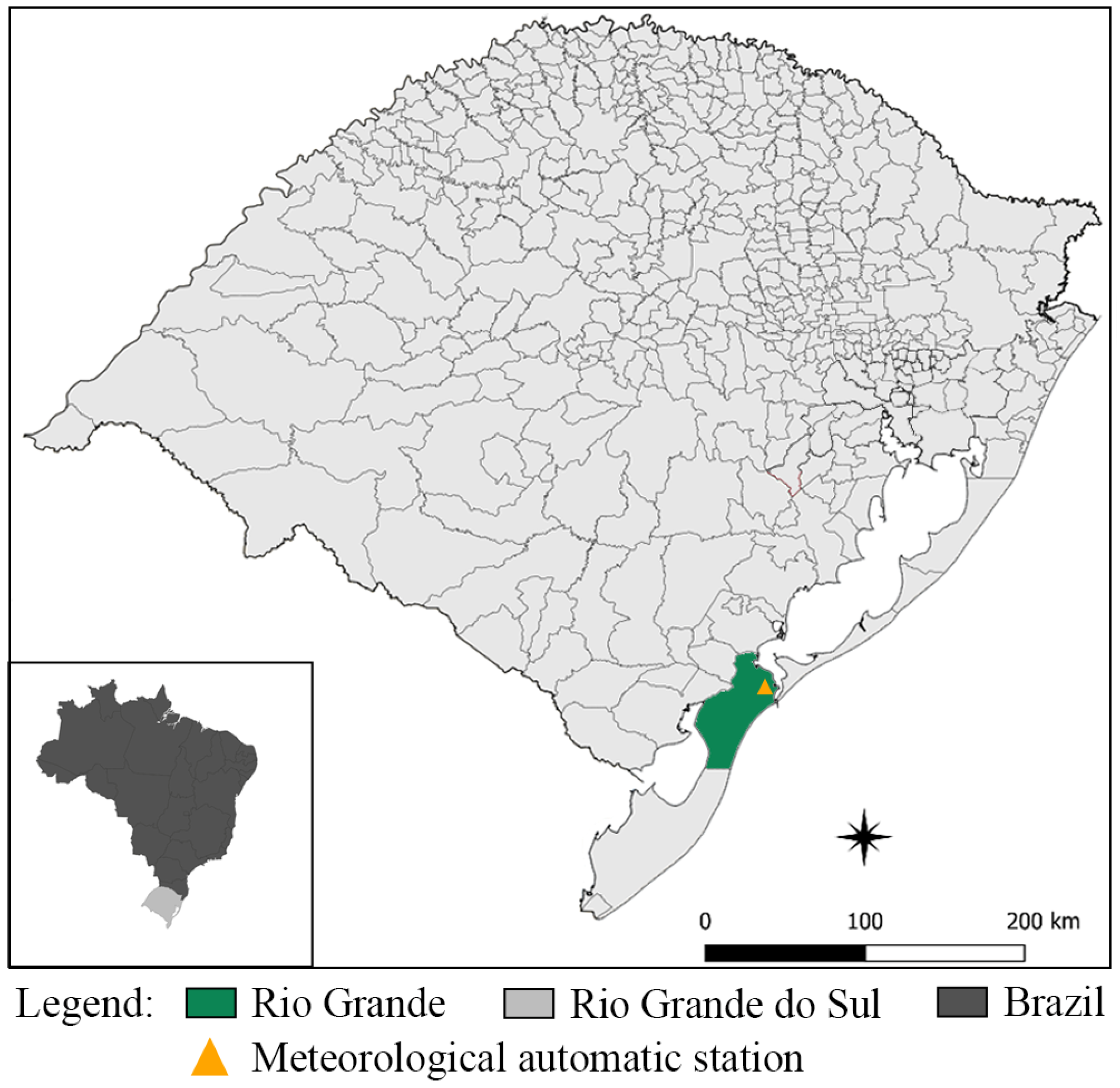
2.1. Study Area

Rio Grande (32°1′60″ S, 52°5′55″ W) is the oldest city in the state of Rio Grande do Sul (RS), Brazil. It is located on the southern bank of the estuary, which channels waters from the Patos Lagoon and its tributaries to the Atlantic Ocean (Figure 1). Spanning an area of 2682.87 km², it has an estimated population of 191,900 inhabitants, according to the Brazilian Institute of Geography and Statistics (IBGE, from Portuguese Instituto Brasileiro de Geografia e Estatística) [37]. Rio Grande hosts one of Brazil’s principal ports—Porto do Rio Grande—positioning port activities as a key economic driver for the city. During the 1970s, 1980s, and 1990s, Rio Grande exhibited the highest industrial growth rate in the state, contributing significantly to Rio Grande do Sul’s industrial output [32].
The city’s climate is classified as humid subtropical, defined as Cfa in the Köppen–Geiger climate classification [37], with a strong maritime influence. Winters tend to be relatively cold, whereas summers are mild, yielding a high annual thermal amplitude.

2.2. Data Collection and Monitoring Period

2.2.1. Air Pollutants—O3, PM2.5, and PM10

Surface atmospheric pollutant data (PM10, PM2.5, and O3) were collected from The Weather Channel application (IBM, Armonk, New York, USA), which provides data generated by the Copernicus Atmospheric Monitoring Service (CAMS) at the European Centre for Medium-Range Weather Forecasts (ECMWF). These satellite-derived data have a horizontal spatial resolution of 0.75° × 0.75° (approximately 80 km). The data were systematically collected through web scraping at predetermined times each day during the study period for the city of Rio Grande. To ensure data quality, all extractions were performed at regular intervals by trained personnel. Daily averages were calculated, and pollutant concentrations were expressed in micrograms per cubic meter (µg/m3). The dataset was then organized by day, year, and season for comprehensive analysis, totaling 730 daily records, with no missing data during the evaluation period.
The air pollutant data collection period spanned from 21 December 2021 to 20 December 2023. This two-year window was carefully selected to capture two full seasonal cycles in the Southern Hemisphere—summer (December to March), autumn (March to June), winter (June to September), and spring (September to December). Additionally, this selection aimed to minimize potential COVID-19-related disruptions, thereby ensuring more representative results. In the study region, mobility restriction measures to control COVID-19 transmission were in effect from March 2020 to August 2021, significantly influencing air pollutant levels during that period [38]. Moreover, the availability of air pollutant data in The Weather Channel application only began in 2020. To avoid biases introduced by the impacts of COVID-19 on air quality, the selected study period was deemed necessary and appropriate.
Although satellite data have inherent limitations, such as non-random misclassification, saturation effects, and atmospheric influences, this method was deemed appropriate for this study due to the limited air quality monitoring network in Brazil, particularly in this region. According to Vormittag et al. [39] and a recent evaluation by the Brazilian Institute of Energy and Environment [40], only 1.6% of Brazilian municipalities have air quality monitoring stations, and nearly 41% of these stations are privately operated, restricting public access to their data. During the study period, Rio Grande did not have any publicly available air quality monitoring stations.
To ensure the reliability of satellite-derived pollutant data for the study area, a validation process was performed using ground-based measurements from other cities in the extreme south of Brazil, as reported in a previous study [41]. The validation results demonstrated strong agreement, with coefficient of determination (R2) = 0.831 and root mean square error (RMSE) = 2.256, supporting the accuracy of the dataset used in this study. Furthermore, the use of satellite data for air quality monitoring in remote regions and areas lacking active ground-based monitoring is supported by WHO (2021) [11]. Other authors also support this methodology for regions with sparse ground monitoring networks or no access to sophisticated deterministic models, using data from The Weather Channel application and other meteorological and air quality data sources [42,43].

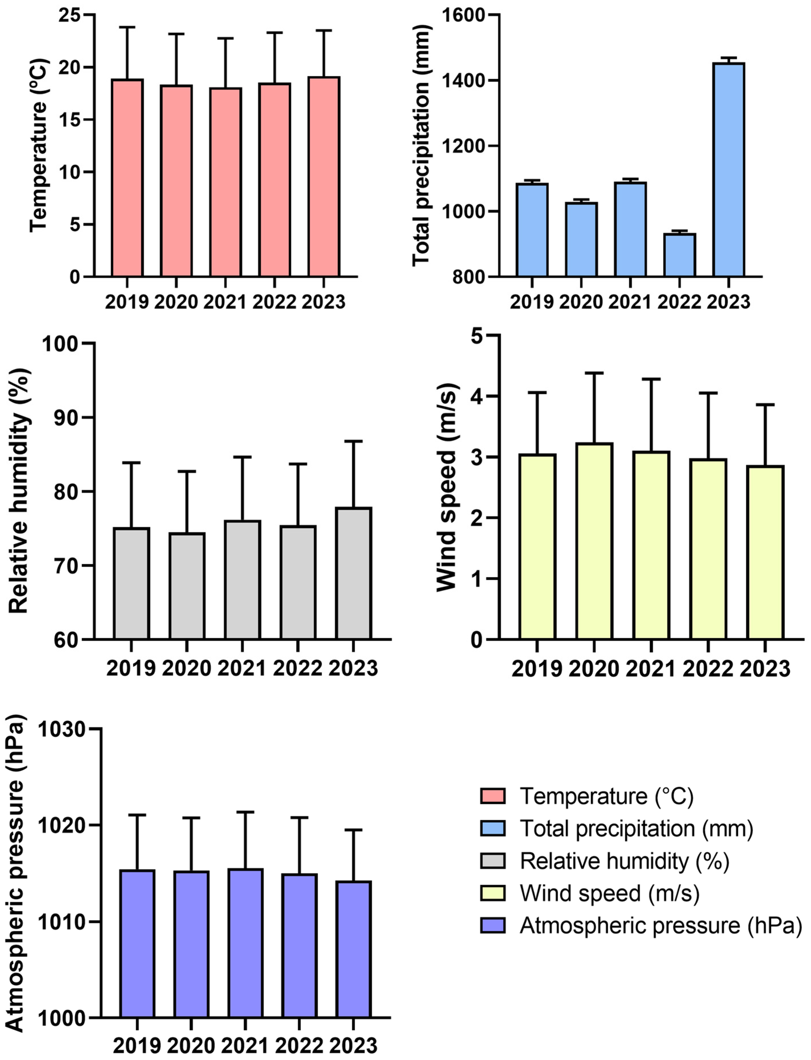
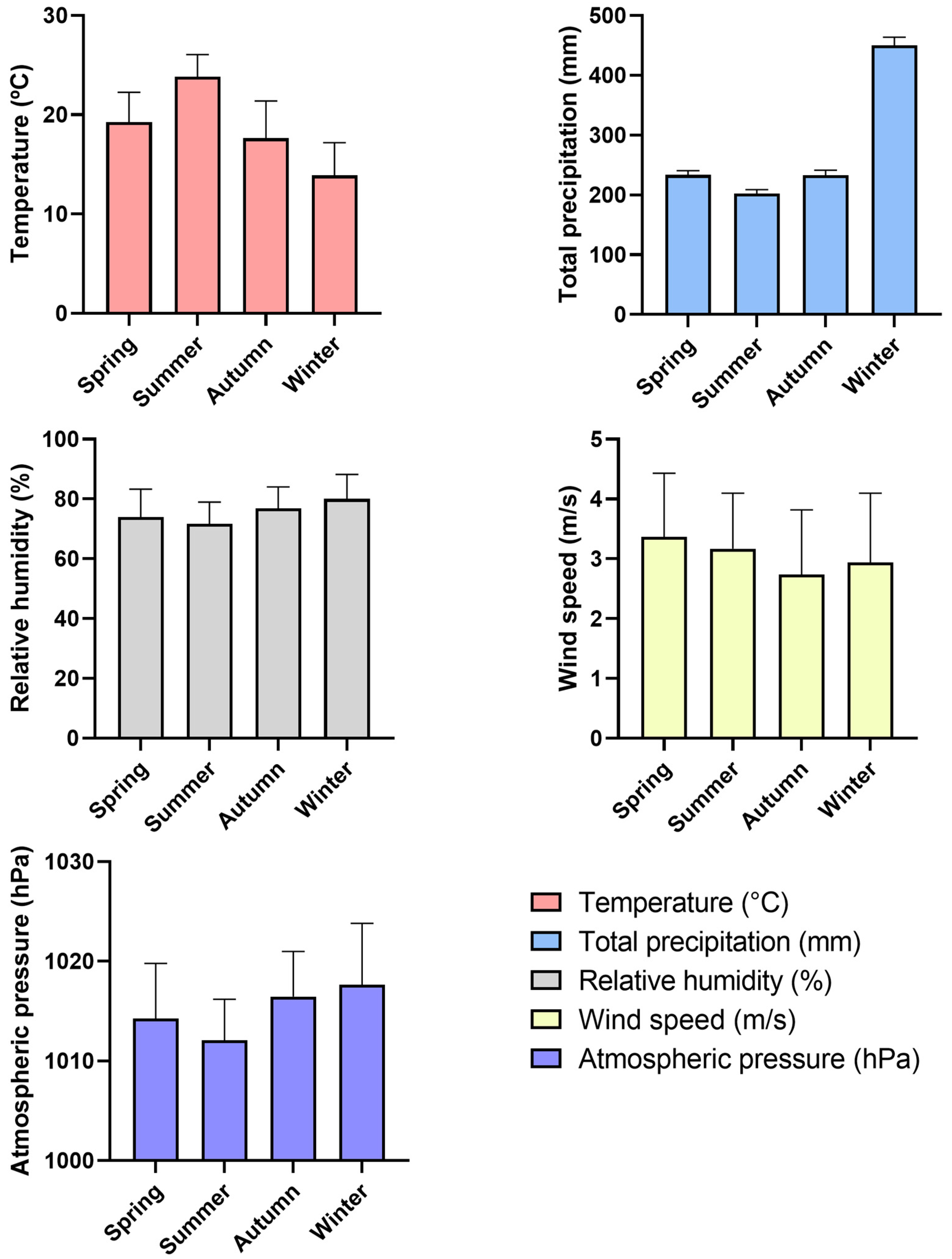
2.2.2. Meteorological Parameters

The monitoring period for surface meteorological variables was performed for a longer period, from 1 January 2019 to 30 December 2023 (five years), as these variables were not directly affected by COVID-19 mobility restrictions, unlike air pollutants. Additionally, using a longer dataset improved the robustness of predictive analyses by providing a more extensive period for model training, enhancing the reliability of statistical associations between meteorological conditions and air pollutant levels.
Surface meteorological variables (surface air temperature, precipitation, air relative humidity, atmospheric pressure, and wind speed) were obtained on a daily basis for Rio Grande from Brazil’s National Institute of Meteorology (INMET). Rio Grande has a single meteorological station, which is an automatic station maintained by INMET, located at 32°04′44″S, 52°10′4″W (Figure 1). This station provides meteorological measurements representative of the entire city area and surrounding regions. Following the retrieval of these daily data, the dataset underwent a strict quality-control process to correct errors or inconsistencies, thereby improving the reliability of subsequent modeling and analysis. The dataset was structured by day, year, and season for detailed assessment.
From the 1826 daily records in the study period, 152 days (8.3%) had missing data for at least one meteorological variable. All available data were used for descriptive analysis and Pearson correlation analysis. However, for the following simulations (Section 2.3), missing data were replaced with the total median value of each respective variable for the corresponding period, ensuring a complete dataset for modeling.

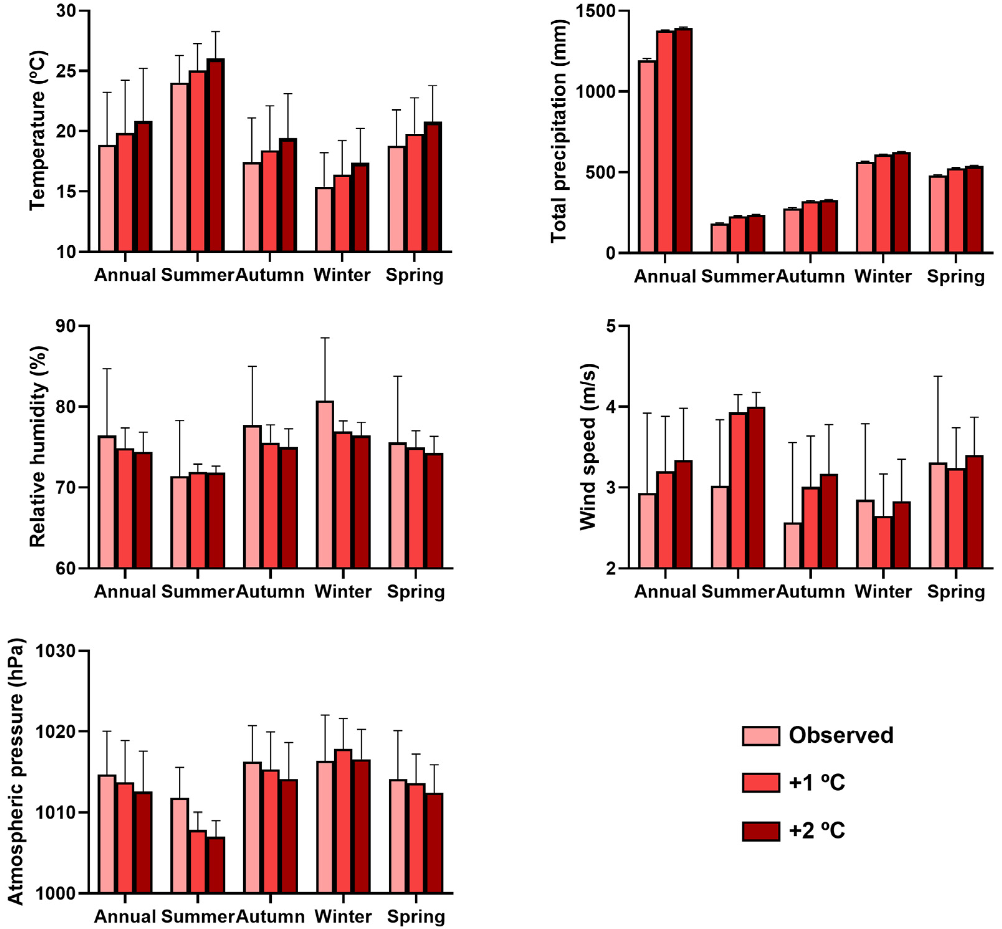
2.3. Scenario Simulations

To estimate projections of pollutant concentrations under warming scenarios, two annual mean temperature-increase thresholds (+1 °C and +2 °C) were selected. These increments align with projections from the Representative Concentration Pathway (RCP) 4.5 scenario proposed by the Intergovernmental Panel on Climate Change (IPCC), which anticipates a +1.4 °C (0.9–2.0 °C) global temperature increase until 2065. By evaluating two increments, this study captures both a moderate warming scenario (+1 °C) and an upper limit within the RCP 4.5 framework (+2 °C).
The simulation process was performed using supervised machine learning algorithms, specifically a Support Vector Machine (SVM) with a radial basis function (RBF) kernel in STATISTICA (version 12.5). This method was selected due to its effectiveness in handling non-linear relationships in environmental datasets, as demonstrated in previous studies on air pollution modeling [30,31]. The kernel parameter gamma was defined as the ratio of the number of dependent variables (continuous dependent) to the number of independent variables (continuous predictors) in the model. Cross-validation was applied throughout the simulations to enhance model robustness and reliability.
The simulation proceeded in two main steps. In the first step, a predictive model of projected atmospheric conditions was generated using historical meteorological data (2019–2023). Meteorological variables—including relative humidity, precipitation, atmospheric pressure, and wind speed—were modeled as dependent variables, while daily temperature increments (+1 °C or +2 °C) in the observed dataset served as the independent variable. Each meteorological variable was modeled individually, using all original observed data from the study period—a total of 1826 daily records—as the training phase. The test phase comprised a corresponding set of 1826 data points, adjusted to reflect the evaluated daily temperature increases. The projected atmospheric scenarios were then generated by combining the increased temperature daily values with the daily predicted meteorological conditions from the test phase of each modeled variable. This process resulted in two distinct atmospheric scenarios, one for +1 °C and another for +2 °C.
In the second step, the predicted meteorological conditions from Step 1 were used as inputs to estimate pollutant concentrations for PM10, PM2.5, and O3 under the temperature increase scenarios. Unlike the meteorological variables, pollutant data were trained using a shorter dataset spanning from the end of 2021 to the end of 2023 (a total of 730 daily records). Following this, similar to the process applied to meteorological variables, each pollutant was individually modeled as a continuous dependent variable, with the predicted meteorological variables from Step 1 (temperature, relative humidity, precipitation, atmospheric pressure, and wind speed) serving as continuous independent variables. It is important to note that the pollutant simulations were trained using the observed meteorological variables for the same period, while the test phase was conducted using the two corresponding years in the projected atmospheric scenarios, with the increased daily temperature and the predicted daily meteorological variables, to ensure coherence in input–output relationships.
To assess model performance, validation was conducted using a subset comprising 10% of the modeled dataset (approximately 182 records for meteorological variables and 62 records for pollutants). These validation records were then compared against observed days with temperature values closest to those of the randomly selected test days, ensuring that model evaluation occurred within the expected temperature range of the warming scenarios. This approach was chosen to validate model performance under the projected conditions rather than against the training dataset, thus avoiding bias and ensuring an independent evaluation. The model performance for meteorological variables presented R2 values ranging from 0.784 to 0.953, with the lowest for precipitation and the highest for wind speed. Temperature was not validated, as it was always used as an independent variable and was not modeled but instead adjusted to reflect the desired temperature increases. For air pollutants, the model performance was as follows: for O3, R2 = 0.883 and RMSE = 5.845; for PM2.5, R2 = 0.824 and RMSE = 3.062; and for PM10, R2 = 0.791 and RMSE = 4.611.

2.4. Data Analysis

All data were organized into Excel spreadsheets. Air pollutant concentrations and meteorological variables, including both observed and modeled data, were subjected to mean and standard deviation calculations at two levels: (i) annual averages for each year in the study period and (ii) seasonal averages, except for precipitation, which was calculated as the total accumulated precipitation for the evaluated period (year or season).
Spearman’s rank correlation coefficient was employed to examine the existence and strength of relationships between observed meteorological variables and air pollutants. This analysis was conducted for the period where air pollutant and meteorological data overlapped. Correlations were considered statistically significant at p < 0.05.
Additionally, a sensitivity and uncertainty analysis was performed to evaluate how variations in key meteorological variables could influence the pollutant concentration projections under the +1 °C and +2 °C warming scenarios. For this analysis, each meteorological parameter—relative humidity, precipitation, wind speed, and atmospheric pressure—was individually perturbed by ±5%, except for atmospheric pressure, which was adjusted by ±2%. The smaller variation applied to atmospheric pressure was chosen due to the magnitude and typical variability range of this variable in the study region. The percentage change in pollutant concentrations resulting from each perturbation was calculated relative to the respective simulated scenario, providing an estimate of the model’s sensitivity to uncertainties in meteorological inputs.
All machine learning and statistical analyses were conducted using STATISTICA 12.5 software. The graphs presented in this study were created using GraphPad Prism 8.

3. Results

The annual averages of meteorological variables for Rio Grande varied over the study period (Figure 2). Mean temperature showed fluctuations, with values ranging from 18.10 °C in 2021 to 19.15 °C in 2023, reflecting interannual variability rather than a defined warming trend. Total annual precipitation was notably higher in 2023, and this, along with the elevated mean temperature in the same year, suggests the strong influence of the El Niño in 2023. Similarly, relative humidity peaked in 2023 (77.91%), possibly reflecting this increase in rainfall. Meanwhile, wind speed exhibited a slight decline over time (3.24 m/s in 2020 to 2.87 m/s in 2023), and atmospheric pressure reached its lowest level in 2023. All the numerical data are presented in Table S1 of the Supplementary Material. These collective changes suggest evolving atmospheric circulation and stability patterns that may have implications for pollutant dispersion and accumulation.
Seasonal data underscore pronounced temperature differences across the year (Figure 3), with summer reaching the highest mean temperature (23.83 °C) and winter the lowest (13.88 °C). Interestingly, winter registered the greatest total precipitation and highest relative humidity (80.06%), whereas summer was the driest season, showing the lowest humidity levels (71.71%). Wind speeds peaked in spring (3.37 m/s), highlighting a period of intensified atmospheric circulation, and reached a minimum in autumn (2.74 m/s). Atmospheric pressure was highest in winter, suggesting more stable atmospheric conditions during that season. All the numerical data are presented in Table S2 of the Supplementary Material.
The annual and seasonal levels of O3, PM10, and PM2.5 are presented in Table 1 and Table 2, respectively. The remote monitoring data for O3, PM10, and PM2.5 indicate clear seasonal patterns. Ozone concentrations were generally highest in winter (64.11 µg/m3) and lowest in summer (54.58 µg/m3). In contrast, PM10 and PM2.5 reached their peak values in spring (14.18 µg/m3 and 8.21 µg/m3, respectively). These variations could be linked to meteorological dynamics, such as temperature inversions or seasonal shifts in humidity. While annual mean levels of O3 and PM10 remained below the final target established by the Brazilian air quality resolution (CONAMA, 2024) [44] and the guideline values of the World Health Organization (WHO, 2021) [11], PM2.5 exceeded both this target and the guideline values of the WHO.
The Spearman rank correlation coefficient revealed that temperature did not show a statistically significant relationship with any of the pollutants under study (Table 3). Precipitation likewise failed to exhibit meaningful correlations with O3, PM10, and PM2.5. Relative humidity, however, displayed a weak but statistically significant positive correlation with O3 (r = 0.36), suggesting that higher ozone levels may co-occur with more humid conditions. While the literature commonly reports that water vapor decreases ozone concentrations, our results indicate a different relationship, likely influenced by local meteorological conditions and specific atmospheric dynamics. Additionally, ozone showed a weak positive correlation with both PM2.5 (r = 0.24) and PM10 (r = 0.17), suggesting possible shared atmospheric conditions favoring their presence.
Atmospheric pressure was positively correlated with PM10 (r = 0.21) and, to a lesser extent, PM2.5 (r = 0.14), potentially indicating that more stable atmospheric conditions favor the accumulation of particles. In contrast, ozone did not exhibit a significant correlation with atmospheric pressure. Wind speed showed no statistically significant correlation with the particulate matter, although ozone had a weak negative association (r = −0.18), suggesting a minor role of wind in ozone dispersion. As expected, PM2.5 and PM10 were strongly correlated with each other (r = 0.98), reflecting their similar physical properties and measurement overlap. This primarily reflects the fact that PM2.5 is a fraction of PM10, and its high variability influences the correlation value.
To explore how a warmer climate might affect local meteorology, two temperature-increase scenarios (+1 °C and +2 °C) were simulated, and the illustrated results are presented in Figure 4. Compared to the observed period (mean temperature of 18.86 °C and total precipitation of 1194.40 mm), the +1 °C scenario yielded a substantial increase in precipitation (1378.20 mm), a slight decrease in relative humidity (74.87%), and a moderate increase in wind speed (3.20 m/s). Atmospheric pressure fell marginally (1013.71 hPa), suggesting a slight shift toward less stable conditions.
Under the +2 °C scenario, these trends became more pronounced. Precipitation reached 1391.33 mm, while relative humidity declined further to 74.42%. Wind speed rose again (3.34 m/s), and atmospheric pressure decreased to 1012.57 hPa. Taken together, these findings imply that a warmer climate in Rio Grande could produce wetter overall conditions, slightly reduced humidity, and higher wind speeds, potentially influencing pollutant dynamics. The numerical results for each scenario are present in the Supplementary Material (Table S3).
With the projected atmospheric conditions, the pollutant concentrations were modeled, and the results are illustrated in Figure 5. In both +1 °C and +2 °C scenarios, the total concentrations of ozone, PM2.5, and PM10 were lower than in the observed period. Although ozone reached its highest observed levels in winter (64.06 µg/m3), it declined to 57.44 µg/m3 (−6.62 µg/m3 reduction) under a +1 °C scenario and to 56.97 µg/m3 (−7.09 µg/m3 reduction) under a +2 °C warming. PM2.5 likewise declined from an observed mean of 7.75 µg/m3 to 6.84 µg/m3 under +1 °C and 6.75 µg/m3 under +2 °C, with the largest drop occurring in summer. PM10 followed a similar pattern, decreasing to 12.63 µg/m3 (+1 °C) and 12.47 µg/m3 (+2 °C), again with the most notable seasonal reductions in summer. The complete numerical values (mean and standard deviation) corresponding to these results are available in Table S4 in the Supplementary Material.
These reductions may stem from the interplay between temperature increases and other meteorological shifts, such as enhanced wind speeds and changes in humidity and precipitation. Nevertheless, the observed decrease in pollutant levels underscores the importance of examining local meteorological responses when projecting air quality in a changing climate.
A sensitivity and uncertainty analysis was conducted to assess the influence of input variability on the pollutant projections. The results indicated that the model was relatively robust. Even under the maximum tested perturbations, changes in particulate matter concentrations remained low, with variations below 1% for all meteorological parameters except atmospheric pressure, which led to maximum changes of 1.97% for PM2.5 and 2.33% for PM10. For ozone, variations exceeded 1% only in response to changes in relative humidity, reaching a maximum of 1.81%. Detailed results of this analysis are presented in the Supplementary Material (Table S5).
The results indicated that the model was relatively robust, with the highest variations observed in PM2.5 and PM10 concentrations in response to changes in atmospheric pressure. Even under the maximum tested perturbation, the changes in pollutant concentrations remained below 2% for O3 and around 2% for particulate matter. Detailed results of this analysis are presented in the Supplementary Material (Table S5).
Furthermore, despite the variations observed in pollutant concentrations under the increased temperature scenarios, these changes did not modify the compliance status of O3 and PM10 with the air quality standards established by CONAMA (2024) and WHO (2021). PM2.5, which already exceeded both the final target of CONAMA (2024) and the guideline values of WHO (2021) in the observed period, remained above these limits even under warming scenarios. This highlights the need for continued air quality management efforts, particularly concerning fine particulate matter, to mitigate potential health risks in a changing climate.

4. Discussion

The results of simulated temperature increase scenarios (+1 °C and +2 °C) in Rio Grande indicated a reduction in both annual and seasonal averages of air pollutants, except for O3 during summer, where its levels increased compared to observed values. These findings contrast with other studies conducted in nearby cities, such as the study by Brum et al. [30] in Dom Pedrito, a small city approximately 300 km from Rio Grande. In their study, the authors investigated the levels of O3, PM10, and PM2.5 under simulated temperature increase scenarios of +2°C and +4°C and observed increases ranging from 7% to 18% in the annual averages of pollutants. Additionally, in the same region, da Silva Bonifácio et al. [31] analyzed the behavior of these same pollutants under simulated +2 °C and +4 °C scenarios in seven cities influenced by coal mining activities (approximately 200 km from Rio Grande), considering both annual and seasonal averages. In almost all scenarios, pollutant levels increased with rising temperatures, except for PM10 and PM2.5 during winter, which showed lower concentrations.
These findings are linked to the absence of a significant correlation between temperature and air pollutants in the study area, which contrasts with patterns observed in other global regions. Globally, temperature influences air pollution through multiple pathways, but local meteorological and geographic factors can modify these relationships [4,5,45,46,47,48]. In Brazil, previous studies in the southern region [30,31] have reported positive associations between rising temperatures and increased air pollutant concentrations. However, these studies were conducted in inland cities, where pollutant dispersion dynamics differ significantly from coastal environments, along with potential differences in local emission sources, which may have contributed to the lack of a correlation observed in this study.
While air pollutants showed no correlation with temperature, other meteorological parameters were associated with pollutant levels: O3 was positively correlated with relative humidity and negatively correlated with wind speed; PM2.5 showed a positive correlation with both relative humidity and atmospheric pressure; and PM10 was positively correlated with atmospheric pressure. The projected reduction in annual mean pollutant concentrations is partially influenced by these correlations. In the projected atmosphere (for both +1 °C and +2 °C scenarios), humidity and atmospheric pressure decreased, and since pollutant levels were significantly and positively correlated with these variables, their concentrations also decreased in the projected scenarios.
The relationship between relative humidity and O3 varies by location. Some studies have reported a non-linear association [49], while others found no significant correlation [50], although the majority of studies report a negative association [51,52]. However, the negative correlation between O3 and humidity is more pronounced in warmer regions with lower relative humidity [53], a condition that differs significantly from the study area, which has annual relative humidity averages exceeding 75%. Regarding PM2.5, several studies have demonstrated a positive relationship between this pollutant and relative humidity [54,55], and reports also indicate that in areas with high humidity, particulate matter can correlate negatively with temperature [56]. The positive association between atmospheric pressure and particulate matter (PM10 and PM2.5) has been documented in various parts of the world [57,58,59].
For a more comprehensive analysis, the present study assessed the seasonal variations in the simulated temperature increase scenarios, revealing that the magnitude of the response was dependent on the season. As Rio Grande has a humid subtropical climate, it experiences cold days in winter and hot days in summer, with an average seasonal temperature difference exceeding 10 °C [60]. In the simulated scenarios, O3 levels were higher than the observed values only in winter. In winter, precipitation rises substantially, relative humidity declines, and these concurrent changes—along with shifts in wind speed and atmospheric pressure—may alter local chemical pathways that promote ozone formation. Consequently, even though temperature itself does not directly correlate with O3, the combined modifications in meteorological parameters appear to favor elevated ozone levels in winter under warmer conditions.
Research that predicts the behavior of meteorological variables and air pollutants under warming scenarios is crucial for informing pollution control policies and climate change mitigation strategies, aiming to maintain environmental quality and public well-being. Recent studies have reported an increase in maximum and mean temperatures in Rio Grande of 1.38 °C and 0.36 °C, respectively, since 1980 [61]. This trend underscores the importance of studies like the present one in understanding local atmospheric dynamics.
Despite its contributions, this study has some limitations. The analysis of meteorological variables was based on data from a single automatic monitoring station over a relatively short period, which may not fully capture long-term trends in meteorological conditions. Meanwhile, air pollutant data were obtained from satellite-derived sources, which, despite providing spatial coverage, are subject to inherent uncertainties, which may include non-random classification errors, saturation effects, and atmospheric effects that can lead to deviations from accurate ground-based data. Although this timeframe includes five years of meteorological data and two years of air quality data, interannual variability and longer-term climate trends may introduce uncertainties in the extrapolation of results. Additionally, machine learning was employed to predict air pollutant behavior under warming scenarios, a method that has been widely used in air quality research [9]. However, the models assume a gradual increase in temperature of +1 °C and +2 °C without considering the potential for non-linear climate responses or feedback mechanisms, such as changes in synoptic-scale meteorological patterns, land-use modifications, or shifts in emission sources that could alter air pollution dynamics. Furthermore, the models used to simulate these warming scenarios rely on present-day relationships between meteorological variables and air pollutants, which may evolve over time due to climate-driven alterations in atmospheric chemistry and transport processes. Another relevant uncertainty stems from the fact that extreme weather events, such as heat waves or intense storms, are not explicitly accounted for in the simulations despite their potential to significantly influence air quality.
Another important limitation is the lack of detailed data on local and regional emission sources. Although Rio Grande has characteristics that favor pollutant dispersion, the contribution of specific sources, such as industrial emissions and vehicular traffic, was not deeply analyzed. Variability in emission patterns over time, including possible changes in anthropogenic sources driven by technological advancements, economic shifts, or regulatory interventions, could impact projected pollutant concentrations in ways that are not fully captured by the current modeling approach. Future studies should incorporate emission inventory data and use high-resolution atmospheric models capable of integrating emission dynamics, meteorological changes, and chemical transformations in a more comprehensive manner. Additionally, expanding the dataset over a longer temporal scale would improve the robustness of trend analyses and help refine projections of air quality under different climate scenarios.

5. Conclusions

This study investigated the relationship between air pollutants (O3, PM10, and PM2.5) and meteorological variables under simulated temperature increase scenarios (+1 °C and +2 °C) in Rio Grande, a medium-sized industrial city in southern Brazil. The results revealed a general decrease in pollutant concentrations under warming scenarios, except for O3 during summer, where levels increased compared to observed values. The absence of a correlation between temperature and pollutant levels in Rio Grande can be attributed to specific meteorological conditions, including the influence of high relative humidity, frequent thermal inversions, and the presence of a VOC-limited ozone production regime.
Understanding how air pollution will evolve under climate change scenarios is essential for designing effective mitigation and adaptation strategies. Given the recent evidence of increasing maximum and mean temperatures in Rio Grande since 1980, this study provides valuable insights into potential projection trends in air pollution in the region. The findings underscore the need for localized approaches to air quality management that consider the complex interplay between meteorological variables and pollutant concentrations.
The results of this study highlight the complexity of air pollution responses to climate change and the necessity of region-specific analyses. By improving predictive models and expanding data collection efforts, policymakers can develop more targeted air quality management strategies to mitigate pollution impacts and protect public health in the context of a changing climate.

Supplementary Materials

The following supporting information can be downloaded at: https://www.mdpi.com/article/10.3390/atmos16040363/s1, Table S1. Annual mean (± standard deviation) of meteorological variables in Rio Grande during the study period (2019–2023); Table S2. Seasonal mean (± standard deviation) of meteorological variables in Rio Grande during the study period (2019–2023); Table S3. Observed meteorological variables during the study period and predicted values under +1 °C and +2 °C warming scenarios; Table S4. Observed pollutant concentrations during the study period and predicted concentrations under +1 °C and +2 °C warming scenarios. Table S5. Sensitivity and uncertainty analysis showing percentage changes in pollutant concentrations (O3, PM2.5, and PM10) due to variations in meteorological parameters under +1 °C and +2 °C scenarios.

Author Contributions

Conceptualization, R.A.T., D.F.d.N. and F.M.R.d.S.J.; methodology, R.A.T., D.F.d.N., G.d.O.S., G.M.G.V.d.A., R.d.L.B. and A.d.S.B.; software, R.A.T., D.F.d.N., R.A.M., L.W.B., R.B., D.F.A. and F.M.R.d.S.J.; validation, R.A.T., D.F.d.N., R.A.M., L.W.B., R.B., D.F.A. and F.M.R.d.S.J.; formal analysis, R.A.T., D.F.d.N., G.d.O.S., G.M.G.V.d.A., R.d.L.B. and A.d.S.B.; investigation, R.A.T., D.F.d.N., G.d.O.S., G.M.G.V.d.A., R.d.L.B. and A.d.S.B.; resources, F.M.R.d.S.J.; data curation, R.A.T., D.F.d.N., R.A.M., L.W.B., R.B., D.F.A. and F.M.R.d.S.J.; writing—original draft preparation, R.A.T., D.F.d.N. and F.M.R.d.S.J.; writing—review and editing, R.A.T. and F.M.R.d.S.J.; visualization, R.A.T., D.F.d.N., G.d.O.S., G.M.G.V.d.A., R.d.L.B., A.d.S.B., R.A.M., L.W.B., R.B., D.F.A. and F.M.R.d.S.J.; supervision, F.M.R.d.S.J.; project administration, F.M.R.d.S.J.; funding acquisition, F.M.R.d.S.J. All authors have read and agreed to the published version of the manuscript.

Funding

This research was funded by the Coordenação de Aperfeiçoamento de Pessoal de Nível Superior—Brazil (CAPES)—Finance Code 001, Fundação de Amparo à Pesquisa do Estado de São Paulo (FAPESP; grant 2024/02579-0 (RAT)), Conselho Nacional de Desenvolvimento Científico e Tecnológico—Research Productivity Fellowship (grant 307791/2023-8 (FMRSJ)), Fundação de Amparo à Pesquisa do Estado do Rio Grande do Sul (FAPERGS; grant 21/2551-0001981-6), and Conselho Nacional de Desenvolvimento Científico e Tecnológico (grant 444528/2023-7 (FMRSJ)).

Institutional Review Board Statement

Not applicable.

Informed Consent Statement

Not applicable.

Data Availability Statement

The data presented in this study are available in the respective references. The raw dataset of air pollution and meteorological variables supporting the conclusions of this article will be made available by the authors upon request.

Acknowledgments

The authors thank the Universidade Federal do Rio Grande (FURG) for the availability of data and logistical support for carrying out the research.

Conflicts of Interest

The authors declare no conflicts of interest.

References

  1. Hoegh-Guldberg, O.; Jacob, D.; Taylor, M.; Guillén Bolaños, T.; Bindi, M.; Brown, S.; Camilloni, I.A.; Diedhiou, A.; Djalante, R.; Ebi, K.; et al. The human imperative of stabilizing global climate change at 1.5 C. Science 2019, 365, eaaw6974. [Google Scholar] [CrossRef]
  2. de Moura, F.R.; da Silva Júnior, F.M.R. 2030 Agenda: Discussion on Brazilian priorities facing air pollution and climate change challenges. Environ. Sci. Pollut. Res. 2023, 30, 8376–8390. [Google Scholar] [CrossRef]
  3. Jarvis, A.; Forster, P.M. Estimated human-induced warming from a linear temperature and atmospheric CO2 relationship. Nat. Geosci. 2024, 17, 1222–1224. [Google Scholar] [CrossRef]
  4. Lou, J.; Wu, Y.; Liu, P.; Kota, S.H.; Huang, L. Health effects of climate change through temperature and air pollution. Curr. Pollut. Rep. 2019, 5, 144–158. [Google Scholar] [CrossRef]
  5. Orru, H.; Ebi, K.L.; Forsberg, B. The interplay of climate change and air pollution on health. Curr. Environ. Health Rep. 2017, 4, 504–513. [Google Scholar] [CrossRef]
  6. Chen, Z.; Xie, X.; Cai, J.; Chen, D.; Gao, B.; He, B.; Cheng, N.; Xu, B. Understanding meteorological influences on PM2.5 concentrations across China: A temporal and spatial perspective. Atmos. Chem. Phys. 2018, 18, 5343–5358. [Google Scholar] [CrossRef]
  7. Zhang, S.; Breitner, S.; Stafoggia, M.; De’Donato, F.; Samoli, E.; Zafeiratou, S.; Katsouyanni, K.; Rao, S.; Palomares, A.D.-L.; Gasparrini, A.; et al. Effect modification of air pollution on the association between heat and mortality in five European countries. Environ. Res. 2024, 263, 120023. [Google Scholar] [CrossRef]
  8. Alahmad, B.; Khraishah, H.; Althalji, K.; Borchert, W.; Al-Mulla, F.; Koutrakis, P. Connections between air pollution, climate change, and cardiovascular health. Can. J. Cardiol. 2023, 39, 1182–1190. [Google Scholar] [CrossRef]
  9. Balogun, A.L.; Tella, A.; Baloo, L.; Adebisi, N. A review of the inter-correlation of climate change, air pollution and urban sustainability using novel machine learning algorithms and spatial information science. Urban Clim. 2021, 40, 100989. [Google Scholar] [CrossRef]
  10. Yan, M.; Li, T. A Review of the Interactive Effects of Climate and Air Pollution on Human Health in China. Curr. Environ. Health Rep. 2024, 11, 102–108. [Google Scholar] [CrossRef]
  11. World Health Organization. WHO Global Air Quality Guidelines: Particulate Matter (PM2.5 and PM10), Ozone, Nitrogen Dioxide, Sulfur Dioxide and Carbon Monoxide; World Health Organization: Geneva, Switzerland, 2021. [Google Scholar]
  12. Tavella, R.A.; Penteado, J.O.; de Lima Brum, R.; da Silva Bonifácio, A.; San Martin, M.C.; Saes-Silva, E.; Brum, A.N.; Buffarini, R.; Filho, W.L.F.C.; Adamatti, D.F.; et al. An exploratory study on the association between air pollution and health problems (ICD-10) with an emphasis on respiratory diseases. Atmos. Pollut. Res. 2025, 16, 102377. [Google Scholar] [CrossRef]
  13. Khomenko, S.; Cirach, M.; Pereira-Barboza, E.; Mueller, N.; Barrera-Gómez, J.; Rojas-Rueda, D.; de Hoogh, K.; Hoek, G.; Nieuwenhuijsen, M. Premature mortality due to air pollution in European cities: A health impact assessment. Lancet Planet. Health 2021, 5, e121–e134. [Google Scholar] [CrossRef]
  14. Badida, P.; Krishnamurthy, A.; Jayaprakash, J. Meta analysis of health effects of ambient air pollution exposure in low-and middle-income countries. Environ. Res. 2023, 216, 114604. [Google Scholar] [CrossRef]
  15. Kim, K.H.; Kabir, E.; Kabir, S. A review on the human health impact of airborne particulate matter. Environ. Int. 2015, 74, 136–143. [Google Scholar] [CrossRef]
  16. Manisalidis, I.; Stavropoulou, E.; Stavropoulos, A.; Bezirtzoglou, E. Environmental and health impacts of air pollution: A review. Front. Public Health 2020, 8, 14. [Google Scholar] [CrossRef]
  17. Holm, S.M.; Balmes, J.R. Systematic review of ozone effects on human lung function, 2013 through 2020. Chest 2022, 161, 190–201. [Google Scholar] [CrossRef]
  18. Xie, Y.; Dai, H.; Zhang, Y.; Wu, Y.; Hanaoka, T.; Masui, T. Comparison of health and economic impacts of PM2.5 and ozone pollution in China. Environ. Int. 2019, 130, 104881. [Google Scholar] [CrossRef]
  19. Mukherjee, A.; Agrawal, M. A global perspective of fine particulate matter pollution and its health effects. Rev. Environ. Contam. Toxicol. 2018, 244, 5–51. [Google Scholar] [CrossRef]
  20. Dominski, F.H.; Branco, J.H.L.; Buonanno, G.; Stabile, L.; da Silva, M.G.; Andrade, A. Effects of air pollution on health: A mapping review of systematic reviews and meta-analyses. Environ. Res. 2021, 201, 111487. [Google Scholar] [CrossRef]
  21. Samad, A.; Garuda, S.; Vogt, U.; Yang, B. Air pollution prediction using machine learning techniques–an approach to replace existing monitoring stations with virtual monitoring stations. Atmos. Environ. 2023, 310, 119987. [Google Scholar] [CrossRef]
  22. Ravindiran, G.; Rajamanickam, S.; Kanagarathinam, K.; Hayder, G.; Janardhan, G.; Arunkumar, P.; Arunachalam, S.; AlObaid, A.A.; Warad, I.; Muniasamy, S.K. Impact of air pollutants on climate change and prediction of air quality index using machine learning models. Environ. Res. 2023, 239, 117354. [Google Scholar] [CrossRef]
  23. Bellinger, C.; Mohomed Jabbar, M.S.; Zaïane, O.; Osornio-Vargas, A. A systematic review of data mining and machine learning for air pollution epidemiology. BMC Public Health 2017, 17, 907. [Google Scholar] [CrossRef]
  24. Houdou, A.; El Badisy, I.; Khomsi, K.; Abdala, S.A.; Abdulla, F.; Najmi, H.; Obtel, M.; Belyamani, L.; Ibrahimi, A.; Khalis, M. Interpretable machine learning approaches for forecasting and predicting air pollution: A systematic review. Aerosol Air Qual. Res. 2024, 24, 230151. [Google Scholar] [CrossRef]
  25. Isaev, E.; Ajikeev, B.; Shamyrkanov, U.; Kalnur, K.U.; Maisalbek, K.; Sidle, R.C. Impact of climate change and air pollution forecasting using machine learning techniques in Bishkek. Aerosol Air Qual. Res. 2022, 22, 210336. [Google Scholar] [CrossRef]
  26. Maltare, N.N.; Vahora, S. Air Quality Index prediction using machine learning for Ahmedabad city. Digit. Chem. Eng. 2023, 7, 100093. [Google Scholar] [CrossRef]
  27. Liu, C.C.; Lin, T.C.; Yuan, K.Y.; Chiueh, P.T. Spatio-temporal prediction and factor identification of urban air quality using support vector machine. Urban Clim. 2022, 41, 101055. [Google Scholar] [CrossRef]
  28. Leong, W.C.; Kelani, R.O.; Ahmad, Z.J. Prediction of air pollution index (API) using support vector machine (SVM). J. Environ. Chem. Eng. 2020, 8, 103208. [Google Scholar] [CrossRef]
  29. Widyarini, L.; Purnomo, H.D. Air Quality Prediction Using the Support Vector Machine Algorithm. J. Inf. Syst. Inform. 2024, 6, 652–661. [Google Scholar] [CrossRef]
  30. Brum, A.N.; de Lima Brum, R.; da Silva Bonifácio, A.; da Silva Júnior, F.M.R.; Zhang, L. Impact of temperature increase on air pollutants—A case study in a small city in southern Brazil. Case Stud. Chem. Environ. Eng. 2024, 9, 100624. [Google Scholar] [CrossRef]
  31. da Silva Bonifácio, A.; de Lima Brum, R.; Tavella, R.A.; They, N.H.; Nadaleti, W.C.; Coronas, M.V.; Saes-Silva, E.; Brum, A.N.; Buffarini, R.; Filho, W.L.F.C.; et al. Health impact assessment of air pollutants in simulated temperature scenarios in the largest coal mining region of Brazil. Case Stud. Chem. Environ. Eng. 2024, 10, 100923. [Google Scholar] [CrossRef]
  32. Mirlean, N.; Ribeiro Gripp, M.L. Geochemical mapping and environmental indexing of an urban area (Rio Grande, RS). Geochim. Bras. 2018, 32, 199–208. [Google Scholar] [CrossRef]
  33. Instituto Brasileiro de Geografia e Estatística (IBGE), Brazil. Cidades e Estados do País–Rio Grande, Rio Grande do Sul. 2022. Available online: https://cidades.ibge.gov.br/brasil/rs/rio-grande/panorama (accessed on 2 February 2025).
  34. Mirlean, N.; Vanz, A.; Baisch, P. Níveis e origem da acidificação das chuvas na região do Rio Grande, RS. Química Nova 2000, 23, 590–593. [Google Scholar] [CrossRef]
  35. de Lima Brum, R.; Penteado, J.O.; Ramires, P.F.; Tavella, R.A.; Honscha, L.C.; da Silva Freitas, L.; de Moura, F.R.; Bonifácio, A.d.S.; da Silva, V.M.; Silva, L.d.S.d.; et al. Southern Air Project-scientific efforts to monitor and measure the impacts of air pollution in southern Brazil. Soc. Impacts 2024, 4, 100074. [Google Scholar] [CrossRef]
  36. Tavella, R.A.; Fernandes, C.L.F.; Penteado, J.O.; De Lima Brum, R.; Florencio Ramires, P.; Coutelle Honscha, L.; Dos Santos, M.; Volcão, L.M.; Muccillo-Baisch, A.L.; Da Silva Júnior, F.M.R. Unexpected reduction in ozone levels in a mid-size city during COVID-19 lockdown. Int. J. Environ. Health Res. 2022, 32, 1801–1814. [Google Scholar] [CrossRef]
  37. Beck, H.E.; Zimmermann, N.E.; McVicar, T.R.; Vergopolan, N.; Berg, A.; Wood, E.F. Present and future Köppen-Geiger climate classification maps at 1-km resolution. Sci. Data 2018, 5, 180214. [Google Scholar] [CrossRef]
  38. Tavella, R.A.; da Rosa Moraes, N.G.; Aick, C.D.M.; Ramires, P.F.; Pereira, N.; Soares, A.G.; da Silva Júnior, F.M.R. Weekend effect of air pollutants in small and medium-sized cities: The role of policies stringency to COVID-19 containment. Atmos. Pollut. Res. 2023, 14, 101662. [Google Scholar] [CrossRef]
  39. Vormittag, E.D.M.P.D.A.; Cirqueira, S.S.R.; Wicher, H.; Saldiva, P.H.N. Análise do monitoramento da qualidade do ar no Brasil. Estud. Avançados 2021, 35, 7–30. [Google Scholar] [CrossRef]
  40. Instituto de Energia e Meio Ambiente (IEMA), Brazil. Dimensionamento da Rede Básica de Monitoramento da Qualidade do Ar no Brasil–Cenários Iniciais. 2021. Available online: https://energiaeambiente.org.br/produto/dimensionamento-da-rede-basica-de-monitoramento-da-qualidade-do-ar-no-brasil-cenarios-iniciais (accessed on 4 March 2025).
  41. Santos, J.E.K.; Tavella, R.A.; de Lima Brum, R.; Ramires, P.F.; da Silva, L.D.S.; Filho, W.L.F.C.; Nadaleti, W.C.; Correa, E.K.; da Silva Júnior, F.M.R. PM2.5/PM10 ratios in southernmost Brazilian cities and its relation with economic contexts and meteorological factors. Environ. Monit. Assess. 2025, 197, 191. [Google Scholar] [CrossRef]
  42. Mejía, D.; Faican, G.; Zalakeviciute, R.; Matovelle, C.; Bonilla, S.; Sobrino, J.A. Spatio-temporal evaluation of air pollution using ground-based and satellite data during COVID-19 in Ecuador. Heliyon 2024, 10, e28152. [Google Scholar] [CrossRef]
  43. Alvarado, M.J.; McVey, A.E.; Hegarty, J.D.; Cross, E.S.; Hasenkopf, C.A.; Lynch, R.; Kennelly, E.J.; Onasch, T.B.; Awe, Y.; Sanchez-Triana, E.; et al. Evaluating the use of satellite observations to supplement ground-level air quality data in selected cities in low-and middle-income countries. Atmos. Environ. 2019, 218, 117016. [Google Scholar] [CrossRef]
  44. Conselho Nacional do Meio Ambiente (CONAMA), Brazil. Estabelece Padrões Nacionais de Qualidade do ar e Fornece Diretrizes Para sua Aplicação. Available online: https://conama.mma.gov.br/index.php?option=com_sisconama&view=atonormativo&id=756 (accessed on 4 March 2025).
  45. Balogun, A.L.; Tella, A. Modelling and investigating the impacts of climatic variables on ozone concentration in Malaysia using correlation analysis with random forest, decision tree regression, linear regression, and support vector regression. Chemosphere 2022, 299, 134250. [Google Scholar] [CrossRef] [PubMed]
  46. Borhani, F.; Shafiepour Motlagh, M.; Stohl, A.; Rashidi, Y.; Ehsani, A.H. Tropospheric Ozone in Tehran, Iran, during the last 20 years. Environ. Geochem. Health 2021, 44, 3615–3637. [Google Scholar] [CrossRef] [PubMed]
  47. Wang, L.; Zhao, B.; Zhang, Y.; Hu, H. Correlation between surface PM2.5 and O3 in eastern China during 2015–2019: Spatiotemporal variations and meteorological impacts. Atmos. Environ. 2023, 294, 119520. [Google Scholar] [CrossRef]
  48. Kirešová, S.; Guzan, M. Determining the correlation between particulate matter PM10 and meteorological factors. Eng 2022, 3, 343–363. [Google Scholar] [CrossRef]
  49. Li, N.; Zhou, T.; Liu, X.; Xu, M.; Li, H. Characteristics of ozone pollution and its relationship with meteorological factors in Langfang City. J. Environ. Eng. Technol. 2021, 11, 217–225. [Google Scholar] [CrossRef]
  50. Chao, C.; Min, B.W. Correlation analysis of atmospheric pollutants and meteorological factors based on environmental big data. Int. J. Contents 2022, 18, 17–26. [Google Scholar] [CrossRef]
  51. de Souza, A.; Kovač-Andrić, E.; Matasović, B.; Marković, B. Assessment of ozone variations and meteorological influences in west Center of Brazil, from 2004 to 2010. Water Air Soil Pollut. 2016, 227, 313. [Google Scholar] [CrossRef]
  52. Carbo-Bustinza, N.; Belmonte, M.; Jimenez, V.; Montalban, P.; Rivera, M.; Martínez, F.G.; Mohamed, M.M.H.; De La Cruz, A.R.H.; da Costa, K.; López-Gonzales, J.L. A machine learning approach to analyse ozone concentration in metropolitan area of Lima, Peru. Sci. Rep. 2022, 12, 22084. [Google Scholar] [CrossRef]
  53. Li, M.; Yu, S.; Chen, X.; Li, Z.; Zhang, Y.; Wang, L.; Liu, W.; Li, P.; Lichtfouse, E.; Rosenfeld, D.; et al. Large scale control of surface ozone by relative humidity observed during warm seasons in China. Environ. Chem. Lett. 2021, 19, 3981–3989. [Google Scholar] [CrossRef]
  54. Zender-Świercz, E.; Galiszewska, B.; Telejko, M.; Starzomska, M. The effect of temperature and humidity of air on the concentration of particulate matter-PM2.5 and PM10. Atmos. Res. 2024, 312, 107733. [Google Scholar] [CrossRef]
  55. Emekwuru, N.; Ejohwomu, O. Temperature, humidity and air pollution relationships during a period of rainy and dry seasons in Lagos, West Africa. Climate 2023, 11, 113. [Google Scholar] [CrossRef]
  56. Vaishali; Verma, G.; Das, R.M. Influence of temperature and relative humidity on PM2.5 concentration over Delhi. MAPAN 2023, 38, 759–769. [Google Scholar] [CrossRef]
  57. Huang, F.; Li, X.; Wang, C.; Xu, Q.; Wang, W.; Luo, Y.; Tao, L.; Gao, Q.; Guo, J.; Chen, S.; et al. PM2.5 spatiotemporal variations and the relationship with meteorological factors during 2013-2014 in Beijing, China. PLoS ONE 2015, 10, e0141642. [Google Scholar] [CrossRef]
  58. Li, X.; Ma, Y.; Wang, Y.; Liu, N.; Hong, Y. Temporal and spatial analyses of particulate matter (PM10 and PM2.5) and its relationship with meteorological parameters over an urban city in northeast China. Atmos. Res. 2017, 198, 185–193. [Google Scholar] [CrossRef]
  59. Kermani, M.; Jafari, A.J.; Gholami, M.; Fanaei, F.; Arfaeinia, H. Association between meteorological parameter and PM2.5 concentration in Karaj, Iran. Int. J. Environ. Health Eng. 2020, 9, 4. [Google Scholar]
  60. Reboita, M.S.; Kruche, N. Normais climatológicas provisórias de 1991 a 2010 para Rio Grande, RS. Rev. Bras. Meteorol. 2018, 33, 165–179. [Google Scholar] [CrossRef]
  61. Reis, Í.S.; da Rosa Silva, T.; Klering, E.; da Silva Lindemann, D.; Maier, É.L.B. Análise da Variabilidade da Temperatura do Ar em Rio Grande–RS (1913-2016). Rev. Bras. Geogr. Física 2022, 15, 583–601. [Google Scholar] [CrossRef]
Figure 1. Geographical location of Rio Grande in the state of Rio Grande do Sul and in Brazil.
Atmosphere 16 00363 g001
Figure 2. The annual mean values of meteorological variables in Rio Grande during the study period (2019–2023). The height of the bar represents the mean, and the error bars represent the standard deviation.
Atmosphere 16 00363 g002
Figure 3. The seasonal mean values of meteorological variables in Rio Grande during the study period (2019–2023). The height of the bar represents the mean, and the error bars represent the standard deviation.
Atmosphere 16 00363 g003
Figure 4. Meteorological parameters in the observed period and under the +1 °C and +2 °C warming scenarios used for pollutant modeling. The height of the bar represents the mean, and the error bars represent the standard deviation.
Atmosphere 16 00363 g004
Figure 5. Observed pollutant concentrations (µg/m3) during the study period and predicted concentrations under +1 °C and +2 °C warming scenarios. The height of the bar represents the mean, and the error bars represent the standard deviation.
Atmosphere 16 00363 g005
Table 1. Descriptive statistics for atmospheric pollutants O3, PM2.5, and PM10 in Rio Grande during the study period.
ParametersO3
(µg/m3)
PM2.5
(µg/m3)
PM10
(µg/m3)
Mean (±SD)58.69 ± 14.467.75 ± 3.8913.14 ± 6.84
Median58.037.2011.98
Minimum27.691.111.50
Maximum110.1945.2865.11
Table 2. The seasonal mean (± standard deviation) of atmospheric pollutants (O3, PM2.5, and PM10) in Rio Grande during the study period.
SeasonO3
(µg/m3)
PM2.5
(µg/m3)
PM10
(µg/m3)
Spring59.04 ± 13.238.21 ± 3.6414.18 ± 7.03
Summer54.58 ± 18.107.57 ± 4.2512.73 ± 6.90
Autumn56.89 ± 10.857.32 ± 3.6612.45 ± 6.43
Winter64.11 ± 13.067.90 ± 3.9413.23 ± 6.90
Table 3. Pearson correlation coefficients between meteorological variables and atmospheric pollutants in Rio Grande.
TemperaturePrecipitation Relative HumidityWind SpeedAtmospheric PressureO3PM2.5PM10
Temperature −0.16 *−0.30 *0.20 *−0.53 *−0.080.01−0.03
Precipitation−0.16 * 0.33 *0.06−0.17 *0.06−0.07−0.04
Relative humidity−0.30 *0.33 * −0.19 *−0.010.36 *0.12 *0.07
Wind speed0.20 *0.06−0.19 * −0.17 *−0.18 *0.010.03
Atmospheric pressure−0.53 *0.17 *−0.01−0.17 * −0.060.14 *0.21 *
O3−0.09 *0.060.36 *−0.18 *−0.06 0.24 *0.17 *
PM2.50.01−0.070.12 *0.010.14 *0.24 * 0.98 *
PM10−0.03−0.040.070.030.21 *0.17 *0.98 *
* indicates statistically significant correlations (p < 0.05).
Disclaimer/Publisher’s Note: The statements, opinions and data contained in all publications are solely those of the individual author(s) and contributor(s) and not of MDPI and/or the editor(s). MDPI and/or the editor(s) disclaim responsibility for any injury to people or property resulting from any ideas, methods, instructions or products referred to in the content.

