Training a Regulatory Team to Use the Odor Profile Method for Evaluation of Atmospheric Malodors

Abstract

Members of the California Air Resources Board (CARB) participated in the odor profile method (OPM) training program. The OPM is the flavor profile analysis (FPA) standard method applied to air samples. The FPA method is a widely used standard method in drinking water taste and odor evaluations. It was found that pre-screening of potential OPM trainees for anosmia cases was necessary. After odor characteristics were defined by odor references and standardized terminology, the trainees were able to accurately describe single odors. However, the trainees could not always simultaneously perceive all odors within a mixture. Therefore, a method to separate the odors in a mixture should be applied in the future for environmental analysis by the OPM. After a half-day training session every day for a week, a panel could be formed to accurately determine the characteristics of atmospheric odors from various facilities. With the help of an intensity scale defined by sugar solutions, the panel could also report average odor intensity values consistent with the facilities’ operation. However, a high variance of individual intensity values relative to panel average was noted. It was likely caused by the simultaneous presence of multiple odors in the air and a lack of definition of low odor intensity values by sugar solutions. Secondly, lower odor intensities were reported when sampling bags were used for the OPM analysis compared to direct sniffing at the facilities’ fenceline, apparently because of the narrow valve opening of the sampling bags. The feasibility of quick adoption of the OPM by a regulatory team as demonstrated in this study is essential for the OPM to be considered as a method to evaluate atmospheric malodors as the FPA for drinking water analysis.

1. Introduction

The relationship between odor nuisances and health risks can be complicated because individual odorous compounds often occur below their hazard thresholds, yet the cumulative effects may bring risk to nearby receptors [1]. As a result, different approaches are adopted by different jurisdictions around the world to address odor nuisances through air regulations [2]. In some jurisdictions, air regulation policies are primarily centered around health risks and may not specifically address odor nuisances. Regulations in jurisdictions where odor nuisances are addressed often rely on dilution-to-threshold (D/T) values and concentrations of specific odorants such as hydrogen sulfide and ammonia to assess sensorial impact. The D/T value is defined as the number of dilutions needed for a given sample to reach the detection threshold, and it is described in terms of Odor Units (OUs) [3]. It is determined by presenting a panel with diluted sample with odorless air at different dilution ratios through an apparatus such as a dynamic olfactometer. The presentation starts from the highest dilution ratio (the most dilute sample), and the dilution ratio decreases at geometric increments with each presentation. It is recorded for each panelist at each dilution step whether the panelist can perceive the odor of the diluted sample compared to odorless air as the background. The individual D/T value is the geometric mean between the lowest dilution ratio where the panelist cannot differentiate the odor of the diluted sample from odorless air and the highest dilution ratio where the panelist can. The panel D/T value is the geometric mean of all individual D/T values of the panel.

Despite its common application, the D/T value of an odorous sample fails to convey important information for odor control. Specifically, the D/T value does not define the characteristics of odors that can indicate potential odor sources and causative compounds, as well as the intensities and acceptability of odors [4]. Figure 1 by Zhou et al. [5] validates this point by demonstrating that the odor intensities caused by different odorous compounds decrease at different rates upon dilution. Thus, a higher D/T value only indicates a more persistent odor during atmospheric dilution. It does not necessarily mean a stronger odor intensity. Similarly, Vitko et al. [6] observed disproportional reductions between D/T values and odor intensities after treatments of foul air from a wastewater facility’s incoming trunklines. The inefficacy of D/T measurement as the primary method of odor investigations is also acknowledged by some regulatory experts due to lack of information on the odor before it is diluted to its threshold and failure to account for interactions among odorants in a mixture [7]. The D/T value of a malodor source sample can be helpful for calculation of separation distance between emission sources and residential areas using dispersion models and/or empirical equations [8]. However, application of the D/T value to a receptor site as the main odor impact criterion, sometimes even as a surrogate for odor intensity itself, as shown by Bokowa et al. [2], can be misleading.

It is also difficult to take all responsible odorous compounds into consideration by using the concentrations of specific odorous compounds to evaluate odor nuisances. For example, Fisher et al. [9] compiled more than 38 odorants belonging to at least 11 classes emitted from biosolids after anaerobic stabilization and/or dewatering. In this case, it is possible for odor nuisances to persist even if the concentrations of specific odorants used by the air regulation for impact assessment are satisfactory because the causative compounds may not be covered.

Thus, two objectives need to be considered for better evaluation of odor problems. First, the D/T value can used to identify if there is an odor problem. However, the D/T value alone cannot be adopted to fully show malodor impact to a receptor from an odor source. Therefore, a second method is needed to assess sensorial effects, especially the characteristic and intensity (strength), of an odor to fill in the gap. Second, a technique to narrow down the list of possible odorants responsible for odor nuisances preferably to a specific compound group should be adopted and validated. In this way, appropriate instrumental analysis can be applied to identify primary chemical causes of odor nuisances. After identification, proper compound concentration limits can be set for the primary odorants alongside specific compounds already covered by air regulations to control odor nuisances.

One promising technique to achieve the two objectives above is the odor profile method (OPM). The OPM determines the odor characters and intensities in air samples in a consistent manner. The OPM is based on the flavor profile analysis (FPA) as the Standard Method 2170 for water and wastewater examination [10]. The FPA has been applied to describe the characteristics and intensities of tastes and odors in water samples, as reviewed by Suffet et al. [11]. References containing standardized materials are used to define odor characteristics in standardized terminology [10]. A panel is first trained with the odor references to develop the standardized terminology before sniffing and describing a sample’s odor characteristics. This practice addresses the challenge of subjective descriptors, as reviewed by Hawko et al. [12]. As for the intensity of each odor perceived, a seven-point intensity scale anchored to sugar solutions at specific concentrations can be used to ensure objective and consistent intensity reporting [10]. A panel tastes the sugar solutions and compares their taste intensities with the strength of each odor characteristic perceived from a sample to determine its intensity value. Taste and odor intensities can be compared because the sense of odor can be related to the sense of taste, as reviewed by Spence [13]. It should be noted that a single odorant’s odor intensity defined by the seven-point intensity scale is linear with the logarithmic value of its concentration, which is known as the Weber–Fechner Law [14]. Such a relationship was well-exemplified by Zhou et al. [5] using Weber–Fechner curves (Figure 1). Known odor characteristics and their causative chemicals in drinking water reported by previous studies using the FPA were compiled into a drinking water taste and odor wheel [11]. The wheel in turn can help pinpoint the chemicals to look for based on the particular taste and odor characteristics perceived in water. As the odor part of the FPA, the OPM has been used for atmospheric odor evaluation in order to better appreciate sensorial impact and/or streamline subsequent chemical analysis to identify the chemical culprit [4,5,6,15,16,17,18,19,20,21]. Odor wheels in different environmental settings have been put forward to describe airborne malodors (Figure 2A–C), like the drinking water taste and odor wheel.

At present, the OPM has not been adopted as a standard method to define an odor problem for air analysis, although many case studies with the OPM applied have shown proof of concept [4,5,6,15,16,17,18,19,20,21]. A possible approach to accelerate the adoption of the OPM as a standard approach is to have regulatory agencies evaluate odor nuisances by the OPM during onsite environmental monitoring. In this way, the effectiveness of the OPM and how the OPM can be used together with existing standard methods such as the D/T method for more comprehensive odor evaluation can be better understood. Then, maybe the OPM could eventually become a second standard method as the D/T method. However, a regulatory agency must be trained in a short period of time due to its already-existing obligations. Therefore, the objective of this study was to examine the ability of the California Air Resources Board (CARB) as an air quality regulation agency to quickly master the OPM and accurately apply it to evaluate odor nuisances caused by various odorous facilities.

2. Materials and Methods

2.1. Chemicals and Materials

Reference materials for standardization of odor characteristics and intensities—Indole (99+%), methyl tert-butyl ether (MTBE) (99%), dimethyl sulfide (DMS) (99+%), dimethyl disulfide (DMDS) (99%), n-butyric acid (99+%), (+)-limonene (96%) and α-pinene (97%) stabilized with α-tocopherol were purchased from ThermoFisher Scientific (Waltham, MA, USA). In addition, 100 μg/mL (±)-geosmin and 2-MIB solutions in methanol, cumene (≥99.5%), n-octane (≥99%) and cis-3-hexen-1-ol (98%) were purchased from Sigma-Aldrich Inc. (St. Louis, MO, USA). Guaiacol (>98.0%), methyl methacrylate (MMA) (>99.8%) stabilized with 6-tert-butyl-2,4-xylenol and 2-isopropyl-3-methoxypyrazine (IPMP) (>98.0%) were purchased from TCI America (Portland, OR, USA). 1-Butanol (ACS Reagent) was purchased from Baker Chemical Co. (Phillipsburg, NJ, USA). Sodium sulfide nonahydrate (98+%), molecular biology-grade phenol (>95%) and pesticide-grade ethyl acetate (>95%) were purchased from Fisher Scientific (Hanover Park, IL, USA). In addition, 1000 μg/mL methyl mercaptan (MeSH) solution in methanol was purchased from Chem Service, Inc. (West Chester, PA, USA). Cane sugar was purchased from Imperial-Savannah LP (Sugar Land, TX, USA).

Sampling and analysis supplies—One-liter fluorinated ethylene propylene (FEP) sampling bags were purchased from Jensen Inert Products (Coral Springs, FL, USA). Odorless water (Milli-Q water) for odor sample preparation was produced by a Milli-Q water purification system (Millipore-Sigma, Burlington, MA, USA), while flavorless distilled water for sugar solutions was purchased from Kroger Co. (Cincinnati, OH, USA). Disposable polycoated paper cups were purchased from Dart Container Corporation (Mason, MI, USA). All glassware was washed by Liqui-Nox^® critical-cleaning liquid detergent (Jersey City, NJ, USA), hot tap water and Milli-Q water before use.

2.2. Panel Description

Two groups of volunteers from the CARB were trained by the OPM in order to satisfy the potential future need for the OPM analysis in both Northern California and Southern California. The first group was based in Sacramento, CA, (panel S) and was made up of 13 volunteers at the beginning while the second group based in Riverside, CA, (panel R) was made up of 9 volunteers at the beginning. Before the initiation of training, all volunteers except for one in panel R were screened by a University of Pennsylvania Smell Identification Test^® (UPSIT^®) purchased from Sensonics International (Haddon Heights, NJ, USA) to make sure that trainees had the ability to observe odor characteristics and did not suffer from severe microsmia or total anosmia.

2.3. Training Activities

All training activities were designed according to the FPA specified by Standard Method 2170 for drinking water [23]. After sniffing 5~7 odor samples, the trainees were instructed to take a 30-min break in an odorless room to avoid possible fatigue.

2.3.1. Odor Characteristic and Intensity Definition

The odor references and their corresponding odor characteristics in standardized vocabulary, as summarized in

Table 1. The odorous compounds in the odor references and their odor characteristics in standardized vocabulary used for both CARB groups. Each odor reference contained the odorous compound and Milli-Q water for dilution. (* Rotten egg odor was caused by hydrogen sulfide produced by equilibrium of sodium sulfide in water.)

#	Odorous Compound	Odor Characteristic
1	Indole	Fecal
2	Cumene	Solvent
3	MTBE	Sweet Solvent
4	Geosmin	Earthy
5	2-MIB	Musty
6	cis-3-Hexen-1-ol	Grassy
7	DMS	Canned Corn
8	DMDS	Decaying Vegetation
9	Sodium Sulfide *	Rotten Egg
10	n-Butyric Acid	Rancid
11	1-Butanol	Alcohol
12	(+)-Limonene	Lemon
13	MMA	Plastic
14	Phenol	Medicinal
15	Ethyl Acetate	Sweet
16	Guaiacol	Smokey
17	Methyl Mercaptan	Natural Gas
18	α-Pinene	Pine
19	IPMP	Moldy
20	n-Octane	Hydrocarbon

, were selected based upon the Standard Method 2170 [23] and additional odors in air [7]. After screening (Section 2.2), all qualified volunteers sniffed the headspace of the 20 odor references, each containing an odorous compound, as listed in Table 1, diluted by Milli-Q water. The trainees recorded their best odor description of each reference before its odor characteristic in standardized vocabulary was revealed. Then, the participants were instructed to smell the headspace of the 20 odor references again with the standardized vocabulary in mind until they were familiarized with all references. It was expected that both groups could characterize an odor consistently after this activity.

A seven-point scale defined by the taste intensities of cane sugar solutions in distilled water at certain concentrations (

Table 2. Seven-point intensity scale standardized by cane sugar standards [23].

Intensity Value	Odor Strength	Sugar Solution Concentration (%)	Note
0	Odor Free	0	None
1	Threshold	Not Applicable	Detection Threshold
2	Very Weak	Not Applicable	Recognition Threshold
3	Action Level [6]	Not Applicable	The value of 3 is only a threshold for average intensity value, not for individual response. A higher average is expected to be a nuisance problem.
4	Weak	5	None
6	Weak–Moderate	Not Applicable	None
8	Moderate	10	Uncomfortable to Smell for Extended Periods [5]
10	Moderate–Strong	Not Applicable	Very Uncomfortable to Smell for Extended Periods [5]
12	Strong	12	Unbearable to Smell Even for Short Periods [5]

) was used for odor intensity determination. As previously mentioned in Section 1, humans can relate the sense of odor to the sense of taste [13]. The seven-point sugar scale was found to be easier to administer in the field and less variable from one session to another compared to an alternative intensity scale using n-butanol defined by ASTM Method E544-18 [24,25]. All trainees were told to take a sip of distilled water without sugar first and then each sugar solution, starting from the most dilute one. It was expected that trainees would be able to differentiate the change in intensity and give a consistent intensity rating for an odor after this activity.

During all subsequent training and analysis activities, all odor references and sugar solutions were available to the participants upon request. All samples for the subsequent training activities shown below were made of the odorants specified in Table 1 for designated odor characteristics together with Milli-Q water or odorless air for dilution.

2.3.2. Triangle Tests

Two types of triangle tests were conducted during the training process—sensitivity tests and differentiation tests. The odors involved in each triangle test session are shown in

Table 3. The odors applied in each triangle test session.

Test Session	Session A		Session B		Session C		Session D
Test Name	Sensitivity Test #1	Sensitivity Test #2	Differentiation Test #1	Differentiation Test #2	Differentiation Test #1	Differentiation Test #2	Sensitivity Test (Air) * #1	Sensitivity Test (Air) * #2
Odor(s) Presented to Panel S	1 Canned Corn + 2 Odorless	1 Grassy + 2 Odorless	1 Rancid + 2 Solventy	1 Moldy + 2 Grassy	1 Fecal + 2 Alcohol	1 Medicinal + 2 Musty	1 Fecal + 2 Odorless	1 Canned Corn + 2 Odorless
Odor(s) Presented to Panel R	1 Canned Corn + 2 Odorless	1 Grassy + 2 Odorless	1 Rancid + 2 Solventy	1 Moldy + 2 Grassy	1 Fecal + 2 Alcohol	1 Medicinal + 2 Musty	Not Conducted	Not Conducted

* The samples were presented in 1L FEP sampling bags. An odorless sample contained 1L odorless air while an odorous sample was prepared by injection of the odorant specified in Table 1 into a 1L FEP bag full of odorless air and its subsequent evaporation. All other samples were prepared in Milli-Q water.

. During the sensitivity triangle tests, the trainees were presented with two odorless samples together with an odorous sample. The trainees were instructed to pick out and characterize the only odorous sample out of the three samples to demonstrate their ability to detect an odor from the odorless background. During the differentiation triangle test, the trainees were presented with two odorous samples with the same odor together with a sample with another odor. The trainees were instructed to pick out and characterize the sample with the different odor to show their ability to detect the difference in odor characteristics.

Session C was conducted to evaluate the effect of familiarization with the testing procedure during Session B on panel performance. Session D was conducted to examine the difference caused by a change of media from water (Session A) to air in FEP bags.

2.3.3. Mixture Evaluation

As shown by previous studies, multiple odors are likely to co-exist in a single air sample [4,5,6,16,19,20,21]. Therefore, both groups were presented with mixtures containing two, three, or four odors each so that the trainees could learn to identify multiple odors within a mixture simultaneously and then characterize each. A detailed make-up of each mixture is shown in

Table 4. Compositions of mixtures used for training the panelists.

Test Session	Session #1			Session #2			Session #3
Mixture	2 Odors	3 Odors	4 Odors	2 Odors	3 Odors	4 Odors	4 Odors (Air) *
Odor(s) Presented to Panel S	Fecal, Rancid	Canned Corn, Moldy, Rancid	Pine, Lemon, Earthy, Grassy	Not Conducted	Earthy, Moldy, Fecal	Rotten Egg, Canned Corn, Decaying Vegetation, Rancid	Canned Corn, Lemon Rancid, Fecal
Odor(s) Presented to Panel R	Fecal, Rancid	Canned Corn, Moldy, Rancid	Garlic, Earthy, Medicinal, Lemon	Musty, Lemon	Earthy, Moldy, Fecal	Canned Corn, Decaying Vegetation, Fecal, Rancid	Not Conducted

* The sample was prepared by injection of the odorants specified in Table 1 into a 1L FEP bag full of odorless air and their subsequent evaporation. All other samples were prepared in Milli-Q water.

. Session #2 was scheduled after Session #1 to evaluate the effect of familiarization with the testing procedure during the first session on panel performance. Session #3 was conducted to examine the difference caused by a change of media from water (Session #1 and Session #2) to air.

2.4. Performance Validation

After training specified by Section 2.3, the two panels went to various odor-emitting facilities and conducted the OPM analysis at the fenceline of each facility. Two types of OPM analysis, onsite analysis and laboratory analysis with sampling bags, were attempted in order to evaluate potential differences in sensitivity. During onsite analysis, the panelists stood at the fenceline and took a sniff. For laboratory analysis, a sample to be analyzed was collected in a 1L FEP sampling bag using an in-house vacuum sampler and then transported to a laboratory. At the laboratory within 6 h after sampling, each participant opened the FEP sampling bag’s valve, squeezed the bag and took a sniff at the outlet. After sniffing either at the fenceline (onsite analysis) or at the sampling bag’s outlet (laboratory analysis), a panelist wrote down any perceived odor characteristics and the odor intensity value for each perceived odor characteristic. Then, a discussion within the panel was allowed to compare results. Each panelist could re-sniff a sample or change the odor characteristics and their intensities without noting this to the rest of the panel. This approach has been helpful for panel evaluation to help define odor characteristics. When half or more of the panel detected a certain odor characteristic in a sample, the odor’s presence was confirmed, and its character, panel average odor intensity value and standard deviation of individual odor intensity values were recorded.

Table 5. Facilities analyzed for performance validation and any related observation.

Panel	Sample Name	Note
Panel S	Rendering Facility (Morning)	Trucks carrying dead animals were observed at the entrance.
	Rendering Facility (Afternoon)	No truck was present.
	Trash Transfer Station #1	None
	Organic Fertilizer Plant	None
	Landfill	None
	Sewage Treatment Plant #1	None
Panel R	Trash Transfer Station #2	Trucks carrying trash were observed at the entrance.
	Sewage Treatment Plant #2	A truck entered the entrance with unknown load.
	Cattle Farm #1	Cattle were denser and closer to the fenceline compared to cattle farm #2.
	Cattle Farm #2	None

shows the detailed compilation of the facilities analyzed. Validation of panel performance was achieved by comparing confirmed odor characteristics and their panel average intensities to the nature of facility operations and results of previous studies on similar facilities. Finally, an attempt to cross-check panel S laboratory analysis results with laboratory analysis of the same samples by an experienced panel at University of California, Los Angeles, (UCLA) was made, but it failed due to low odor sensitivities observed during laboratory analysis with the sampling bags, as described below in Section 3.4.2.

2.5. Statistical Test

The two-tailed Welch’s t-test was used to evaluate if there was significant difference between two sets of data on average. Examples of a set of data include each trainee’s number of correct response(s) during a test session, each panelist’s reported odor intensity for a specific odor characteristic, etc. It should be noted that the two-tailed Welch’s t-test could not determine which set of data was significantly larger on average. Instead, the one-tailed Welch’s t-test was used to evaluate whether the average value of a set of data was significantly larger or lower than that of another set of data. All Welch’s t-tests were conducted using the online calculator Statistics Kingdom [26].

The significance level for all tests was 0.05. If the p-value reported by a two-tailed Welch’s t-test was lower than the significance level of 0.05, the two sets of data were considered significantly different on average. Similarly, if the p-value reported by a one-tailed Welch’s t-test was lower than the significance level of 0.05, the average value of one set of data was considered to be significantly larger or lower than that of the other set of data on average.

3. Results

3.1. Screening by University of Pennsylvania Smell Identification Test^® (UPSIT^®)

According to criteria set by Doty [27], most volunteers from both groups were found to suffer from mild microsmia, while a single case of total anosmia was identified (

Table 6. UPSIT^® screening results.

Panel	Normosmia Case(s)	Mild Microsmia Case(s)	Moderate Microsmia Case(s)	Severe Microsmia Case(s)	Total Anosmia Case(s)	Total
Panel S	0	12	1	0	0	13
Panel R	2	5	0	0	1	8 *

* One volunteer did not take UPSIT due to limited availability.

). The individual with total anosmia dropped out before training initiation. Therefore, anosmia screening of potential trainees for the OPM using UPSIT^® was effective and necessary. Despite absence from screening, one participant demonstrated average performance during subsequent training and validation processes. Thus, the participant was included as a part of panel R. Finally, two volunteers from panel R did not participate in any of the following activities, though they passed the screening process, due to limited availability. This showed the challenge brought by existing obligations during training at a regulatory agency.

3.2. Odor References and Triangle Tests

Without standardized vocabulary for odor characteristics, both groups gave multiple descriptions for each of the 20 odor references in Table 1. As a result, few matched the vocabulary in Table 1 (Figure 3). Thus, establishment of standardized terminology for odor characteristics expected in the field and its familiarization to the panel were found to be essential for successful panel training for the OPM. Otherwise, it would be impossible to tell whether the vastly diverse descriptions are for the same odor characteristic or for different ones. As a result, calculation of the panel average intensity value and the standard deviation value of individual odor intensity values for each odor characteristic would be impossible.

Both groups of trainees demonstrated their ability to differentiate an odor from the odorless background and from another odor with a different characteristic during triangle tests (Figure 4). This proved the UPSIT^® test was effective. Further, the change of media from water to air (Session D) did not affect the ability of panel S to distinguish an odor from the odorless background (Figure 4A). The average number of correct choice(s) by panelists from panel S during Session A (medium—water) was not significantly from that during Session D (medium—air) based on a two-tailed Welch’s t-test (p = 1 > 0.05). Additionally, Figure 4B showed that the familiarization with the differentiation triangle test’s procedure did not improve either panel’s ability to differentiate between two odor characteristics. The average number of correct choice(s) by panelists from panel S during Session B was not significantly from that during Session C based on a two-tailed Welch’s t-test (p = 1 > 0.05). The same applied to panel R (p = 1 > 0.05). Finally, there was no significant difference between the performance (measured by the average number of correct pick(s)) of panel S and panel R during both the sensitivity triangle test (Session A—p = 0.448 > 0.05) and the differentiation triangle tests (Session B—p = 0.265 > 0.05 and Session C—p = 0.265 > 0.05).

3.3. Odor Perception in Mixtures

Most trainees from both panels could not perceive all odor characteristics within a mixture containing two, three or four different odors. As a result, Figure 5 shows on average the percentage of identified odor characteristics never exceeded 75%.

The change of media from water to air did not seem to affect the performance of panel S in analyzing a mixture of four odors, as shown in Sessions #1~#3; Figure 5C. The average number of correctly identified odor(s) by panel S during Session #1 (medium—water) was not significantly different from that during Session #3 (medium—air) (p = 0.259 > 0.05). The same was true for panel S between Session #2 (medium—water) and Session #3 (medium—air) (p = 0.162 > 0.05).

Familiarization with the mixture evaluation’s procedure could either significantly improve or worsen a panel’s ability to perceive multiple odor characteristics within a mixture. The average number of correctly identified odor(s) from a mixture of four odors by panel S during Session #1 was significantly higher from that during Session #2 conducted after Session #1 (p = 0.015 < 0.05). The same kind of decline in performance after familiarization was also observed for panel R during perception of mixtures with three odors (p = 0.029 < 0.05). However, panel R identified significantly more odors on average from a mixture of four odors after familiarization (p = 0.005 < 0.05). The discrepancy in the effects of familiarization on the perception of odor mixtures may have been caused by the different odors used in the different test sessions (Table 4).

Finally, panel S performed significantly better in many cases than panel R in the analysis of mixtures with two odors (Session #1—p = 0.046 < 0.05), three odors (Session #2—p = 0.009 < 0.05) and four odors (Session #1—p = 0.001 < 0.05). Since there was no significant difference between the two panels during triangle tests where no odor mixtures were involved (Section 3.2), it could be concluded that the ability to identify odors within a mixture was highly variable for different individuals.

3.4. Performance Validation by the OPM Analysis of Facilities

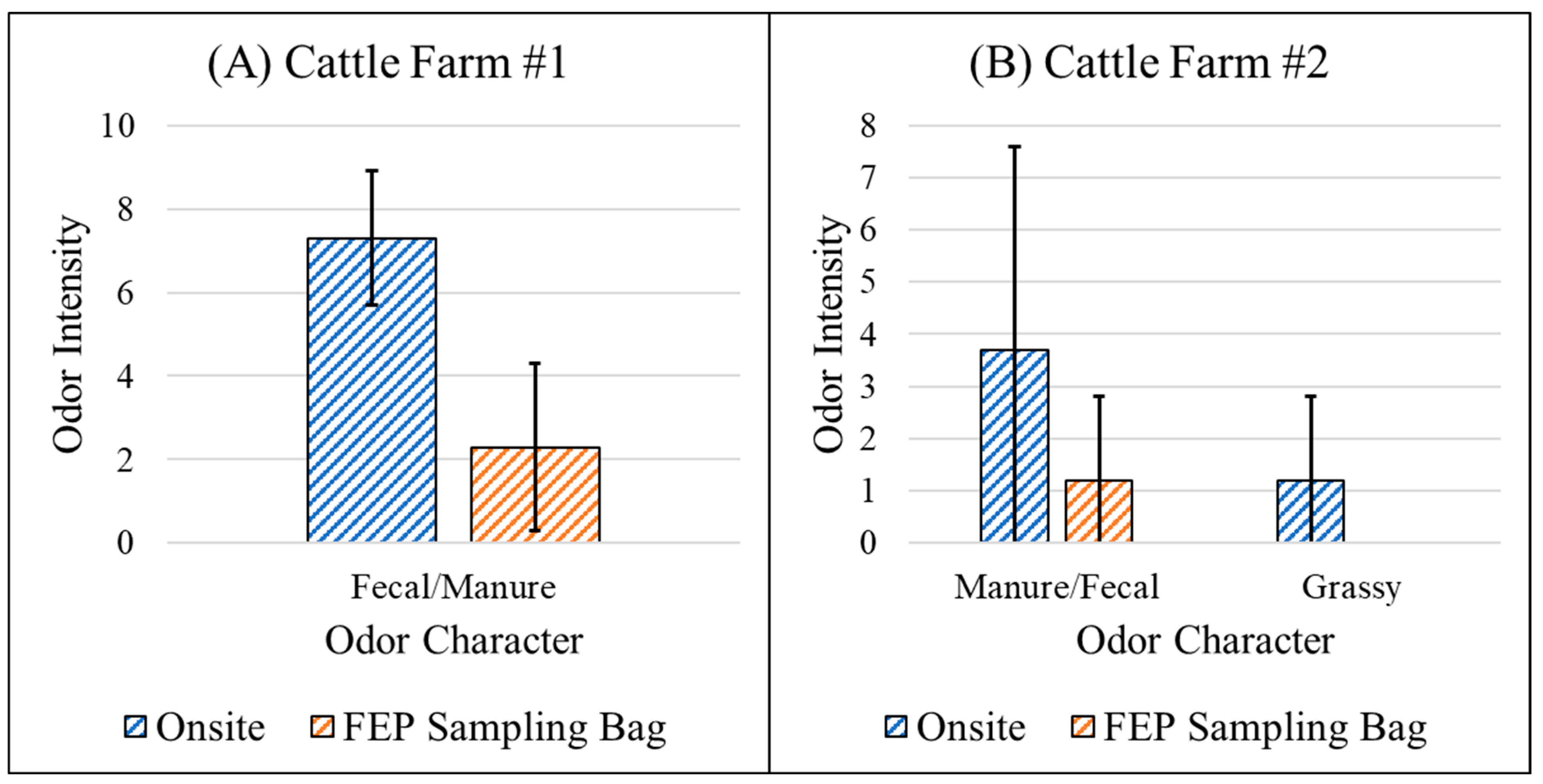
3.4.1. Fenceline Analysis

Figure 6 shows the average and standard deviation values of the confirmed odor characteristics’ odor intensities by both panels at the fenceline of various facilities. No odor was confirmed at the rendering facility in the afternoon and the landfill by panel S. Thus, their results are not included in Figure 6A.

The perception of decaying vegetation odor at the trash transfer station #1 by panel S, as well as rancid and exhaust odors at the trash transfer station #2 by panel R, is consistent with the odors detected by Curren et al. [16] at a trash transfer station. The grassy odor confirmed at the trash transfer station #1 by panel S was probably caused by the background odor of fresh grass cuttings outside the facility.

The fecal odor perceived at both sewage (wastewater) treatment plants and the rotten egg odor perceived at sewage treatment plant #1 were reported by Bian [28], Zhou et al. [5], Vitko et al. [6], Zhou et al. [17] and Gao et al. [21] at wastewater treatment facilities as well. The presence of a chlorine odor at sewage treatment plant #2 was not expected, but it appeared to be related to the tanker truck observed at the plant entrance (Table 5) and/or variations in the chlorination process at the plant.

Despite the lack of previous research involving the OPM analysis of the same types of facilities for reference, the odor characteristics confirmed at the organic fertilizer company (fecal/manure and oil/gasoline/solventy), rendering facility (putrid/dead animal and rancid/sour) and cattle farms (fecal/manure and grassy) were consistent with the nature of the facilities’ operations.

It should be noted that the putrid/dead animal odor characteristic confirmed during the OPM analysis of the rendering facility in the morning by panel S was not any of the odor characteristics with standardized vocabulary that the panel was trained on (Table 1). Panel S could quickly distinguish this particular odor characteristic from all odor characteristics they were trained on and then agreed upon the best odor descriptor by panel discussion thanks to the application of odor references (Table 1) during panel training.

It should be noted that in most cases there was a high variance in individual odor intensity values relative to the panel average odor intensity. It is reflected by the large error bars in Figure 6. However, both panels were still able to report different panel average intensity values that correspond with changes in facility operations. Two specific cases are shown below.

First, panel S confirmed putrid/dead animal and rancid/sour odor characteristics with average intensities of 4.0 and 3.2, respectively, at the fenceline of the rendering facility in the morning (Figure 6A), when trucks carrying dead animals were at the nearby entrance. Meanwhile, neither odor was perceived by the majority of the panel in the afternoon when there was no truck with dead animals at the entrance and all operations were enclosed. In other words, the average intensities dropped to 0 for both odor characteristics since they were not confirmed. One-tailed Welch’s t-tests further confirmed the significantly higher average odor intensities at the rendering facility in the morning than those in the afternoon (putrid/dead animal—p = 0.041 < 0.05; rancid/sour—p = 0.013 < 0.05).

Second, panel R gave a higher panel average odor intensity value for the fecal/manure odor characteristic at the fenceline of cattle farm #1 than that given at the fenceline of cattle farm #2. At the same time, cattle farm #1 had visibly denser cattle population and it was situated closer to the fenceline compared to cattle farm #2. The significantly higher average odor intensity value for the fecal/manure odor characteristic at cattle farm #1 was further confirmed by a one-tailed Welch’s t-test (p = 0.038 < 0.05).

In conclusion, after a week’s simple training, both panels could accurately characterize odors produced by various facilities and react to variations in facility operations by reporting different odor intensities that changed accordingly.

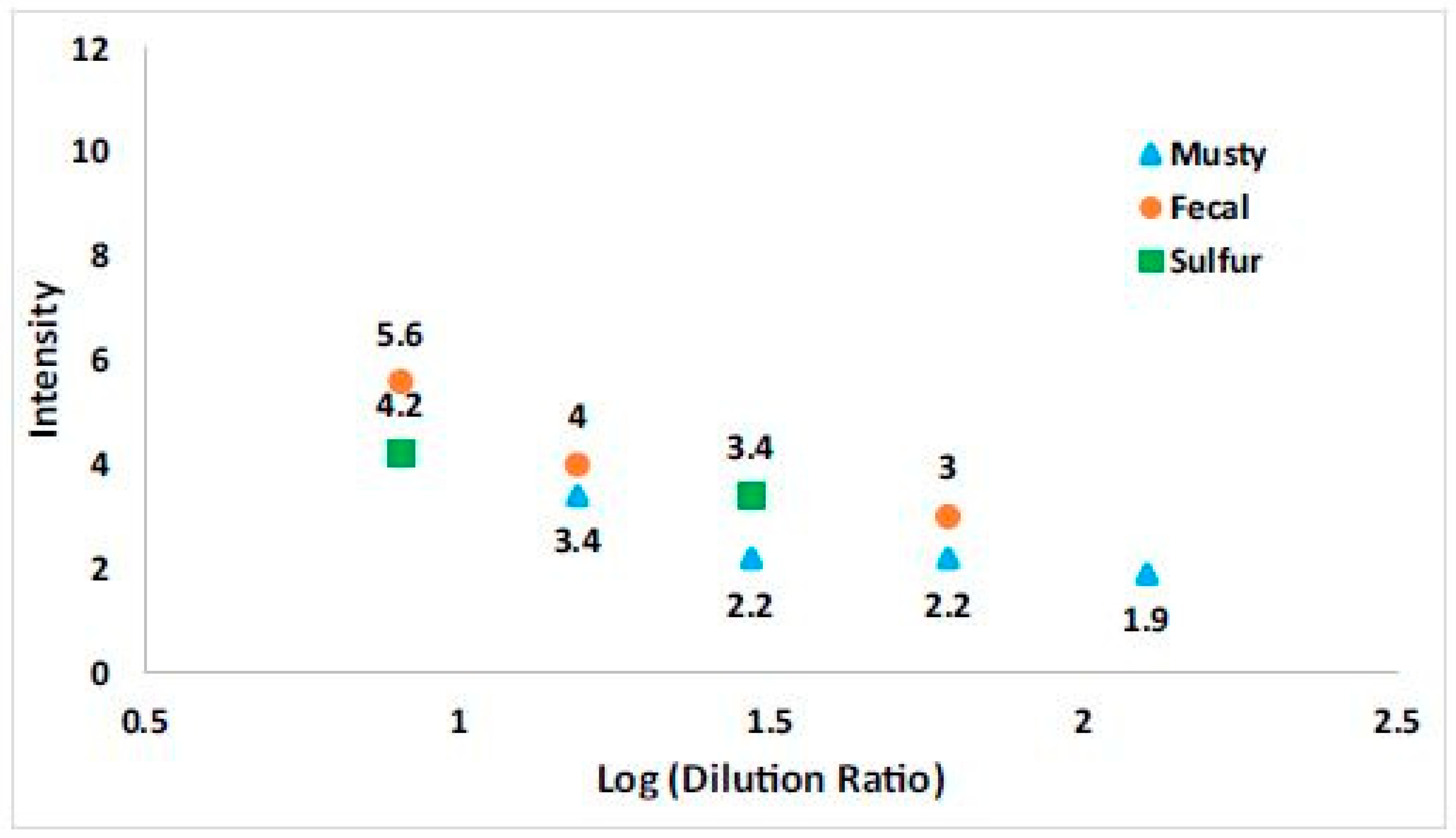
3.4.2. Loss of Sensitivity During Laboratory Analysis

Compared to onsite OPM analysis where panelists sniffed at the fenceline of facilities (Section 3.4.1), few odors were confirmed at the same facilities by laboratory OPM analysis where panelists sniffed from FEP sampling bags with samples collected at the same locations where onsite OPM analysis took place. Figure 7 shows the only two facilities where odor characteristics were confirmed during laboratory analysis using FEP sampling bags. It compares the odor intensities reported by laboratory OPM analysis using FEP sampling bags to the odor intensities reported by onsite OPM analysis. The odor characteristics perceived in both ways matched. However, the average odor intensity of the fecal/manure odor characteristic given by laboratory analysis of cattle farm #1 using FEP sampling bags was significantly lower compared to onsite OPM analysis (p = 0 < 0.05) (Figure 7A). The average odor intensities of the fecal/manure and grassy odor characteristics reported at cattle farm #2 by onsite OPM analysis were higher than those reported by laboratory analysis using FEP sampling bags, though the differences were still not statistically significant (fecal/manure—p = 0.096 > 0.05; grassy—p = 0.063 > 0.05). As for the other facilities in Table 5, no odor characteristic was confirmed at all by laboratory OPM analysis using FEP sampling bags. Therefore, there was a loss of sensitivity issue with the use of FEP sampling bags for laboratory OPM analysis.

4. Discussion

4.1. Perception of Odor Mixtures

The results in Section 3.3 where both panels were limited in their abilities to characterize all odors in a mixture are consistent with the review by Laing and Jinks [29] where it was found that humans could rarely identify more than three odors in a mixture regardless of training, experience, method and odorants. This restraint presents a challenge to airborne malodor analysis due to expectation of co-existing odors in a single sample based on previous studies [4,5,6,16,19,20,21]. More importantly, different odorants have different odor detection threshold concentrations where average human noses can detect their odors and different odor intensity reduction rates upon dilution [5]. As a result, an odorous compound may be masked by the smell of another odorant initially at the emission source due to the latter’s high concentration and odor intensity. However, the smell of the masked odorant may be perceived downwind because its odor intensity decreases more slowly upon atmospheric dilution compared to the other odorant. Thus, the odor characteristics perceived at the emission source may be different from those perceived at downwind receptor sites. The phenomenon is known as the “peeling of an onion effect” and was discussed by Zhou et al. [5] (Figure 8) and Suffet et al. [15] for air samples using the OPM. If the OPM analysis is conducted in a facility (odor emission source) to choose target compounds for monitoring and control based on odor characteristics, the chosen compounds might not be the ones causing odor nuisances downwind due to the “peeling of an onion effect”. Thus, public complaints downwind might persist despite the monitoring and control efforts. Similarly, odor attribution through matching of odor characteristics at downwind receptor sites with those at possible emission sources may also fail due to the “peeling of an onion effect”.

To overcome the limitation, training on olfactometer operation should be conducted in the future. An olfactometer dilutes a given air sample by odorless air at pre-set dilution ratios and presents the diluted flow to a panel for sensory analysis. It was used by Zhou et al. [5] and Bian [28] to dilute odor emission source samples at various dilution ratios and conduct the OPM analysis on the diluted flows. In this way, potential changes of odor emission’s odor characteristics and their odor intensities as it travels downwind could be evaluated by simulating the atmospheric dilution process with dilution of odor emission source samples by odorless air inside an olfactometer. More importantly, the “peeling of an onion effect” could be observed based on changes of odor characteristics with increasing dilution of odor emission source samples with an olfactometer, as exemplified by Zhou et al. [5] (Figure 8).

4.2. High Variance in Individual Odor Intensity Values

Individual odor intensity values reported for each odor characteristic confirmed during onsite OPM analysis of various facilities at the fenceline were found to be highly variable (Section 3.4.1). It was indicated by the large error bars in Figure 6 relative to the panel average odor intensity values. The high variance may have been caused by the panelists’ limited ability to perceive multiple odors within a mixture simultaneously, as discussed in Section 4.1. Since the odor emissions from all the analyzed facilities contained multiple odor characteristics (both confirmed characteristics and odor notes), each panelist could not identify all odor characteristics at each facility. As a result, individual odor intensity values of 0 were reported for all confirmed odor characteristics except for fecal/manure odor at cattle farm #1 because some panelists failed to perceive the odor characteristics at all. These values of 0 increased the variance of the individual odor intensity values. Future research should test the hypothesis by preparation of an air sample with only one odor characteristic and an air sample with the same odor characteristic and other co-existing odor characteristics. The odorant concentrations should be controlled in a way that leads to the same panel average odor intensity values of the shared odor characteristic in both samples. Then, the variance of individual odor intensities reported for the shared odor characteristic can be compared between the two samples.

Another possible reason for the high standard deviation of individual odor intensity values was the lack of sugar solutions to define low intensity values. The lowest intensity value defined by a specific sugar solution on the intensity scale is 4 (Table 2). By comparison, the panel average intensity values of most confirmed odor characteristics were lower than 4 (Figure 6). Since definition by sugar solutions ensured the consistency of reported odor intensity values by the OPM, future research should improve the intensity scale as shown by Table 2 through additional sugar solutions for low intensity values such as 2. After that, it should be evaluated whether the variance of individual odor intensity values could be lowered for odor characteristics with low panel average odor intensities.

The high standard deviation of odor intensity values across panelists compared to the panel average odor intensity value shown by large error bars in Figure 6 is consistent with the finding of Curren et al. [25]. However, Curren et al. [25] also noted less variance of panel average odor intensities across sessions. It should be able to explain why panel average odor intensity values can be used for Weber–Fechner curve fitting as exemplified by Figure 1 in spite of largely different odor intensity values from one panelist to another. It should also explain why panel average odor intensity can be compared with an odor nuisance intensity threshold to determine if public complaints can be expected in drinking water supplies [30,31].

Since panel average odor intensity values are reliable, both panels in this study should still be able to evaluate the extent of odor nuisances based on the panel average odor intensity values determined by the OPM despite high variance in individual odor intensity values. Future research should compare panel average odor intensity values with public complaint data at the same location to evaluate this point.

4.3. Loss of Sensitivity with Sampling Bag Use

The lower odor intensities reported by laboratory OPM analysis by sniffing from FEP sampling bags with collected samples compared to onsite OPM analysis with direct sniffing at the same locations where samples were collected for laboratory analysis are shown by Figure 7. This most likely was caused by the narrow outlet tube attached to the FEP sampling bag valve (Figure 9). As a result, the sample flow out of the bag was restricted and quickly diluted by surrounding air before sniffed by panelists. By comparison, the necks of Erlenmeyer flasks used for holding water samples for odor analysis by the FPA specified by Standard Method 2170 [10] are usually wide enough for sniffing to take place without severe dilution of odorants in the headspace of the samples by surrounding air. Since sniffing from sampling bags has been used for the OPM analysis of environmental samples [6,17], the cause of lower odor sensitivities related to sniffing from sampling bags and potential remedies should be further investigated. A modification of the valve and the outlet tube of the FEP sampling bag to ensure a higher sample flow rate during panel sniffing from bag outlet should be attempted.

4.4. Future Studies

Two panels from CARB as a regulatory agency were trained on the OPM analysis of air samples in a short period of time in order to accelerate the application and maturation of the OPM as an airborne malodor analysis method. It was found that, within a week, a panel could be formed using a simple training procedure. The panel could properly characterize emissions from common odorous facilities both in terms of odor characteristics and odor intensities. However, challenges of significant dropout rates during training processes due to existing obligations of participants, as well as possible cases of anosmia, were noted. Therefore, a large group of volunteers together with screening by UPSIT^® before training would be essential for a successful outcome.

Additionally, limitations observed during analysis of odor mixtures warranted combination of the OPM with the olfactometer so that any initially masked odor at the source capable of causing nuisance downwind due to the “peeling of an onion effect”, as discussed in Section 4.1, could be revealed. Application of the olfactometer may also reduce the high variance of individual odor intensity values relative to the panel average value, since dilution of an odor mixture by the olfactometer separates the most persistent odor characteristic from the others. As discussed in Section 4.2, the co-existence of multiple odor characteristics within each sample and the panelists’ limited ability to perceive them simultaneously likely contributed to the observed high variance. Future training of the panels should involve familiarization with the operation of a dynamic olfactometer and the application of the OPM during the olfactometer operation.

In addition, additional odor references, especially for the putrid/dead animal odor characteristic observed by panel S at the rendering facility (Figure 6A), should be determined and included in the inventory (Table 1). Similarly, additional sugar solutions should be applied to define intensity values lower than 4 to improve the intensity scale (Table 2). In this way, the high standard deviation of individual odor intensity values relative to panel average odor intensity value may be reduced by ensuring more consistent reporting of odor intensities at low values (Section 4.2).

The modifications of sampling bag valves and outlet tubes as shown in Figure 9 should be attempted and validated to increase sample flow rate and limit sample dilution by surrounding air during bag squeezing and panel sniffing. In this way, the low odor sensitivities of laboratory OPM analysis using FEP sampling bags (Section 3.4.2) may be improved. Then it will be necessary to conduct a comparison of the OPM analysis of atmospheric odors onsite versus the new sampling bag configuration.

This study validated a panel’s ability to characterize odors and give varying intensities consistent with operational changes of emission sources with a simple training procedure. Odor characteristics can be used to indicate possible compounds causing odor nuisances and thus determine the proper chemical analysis methods [32]. Meanwhile, odor intensities, especially the panel average values, can be used to determine the extent of sensorial nuisances by comparison with the action level where the odors are expected to cause nuisances (Table 2).

The information gathered by the OPM can then help the establishment of regional concentration limits for odorous compounds to assist odor nuisance evaluation. First, odorants causing nuisances can be identified based on the odor characteristics confirmed by the OPM, and this will help choose the proper chemical analysis method(s). The odorants should be the compounds for which the concentration limits are set. Secondly, the Weber–Fechner curves exemplified by Figure 1 should be determined for the identified odorants to establish the linear relationship between the logarithmic value of each odorant’s concentration and its odor intensity value. Finally, the concentration of each odorant corresponding to the action level (Table 2) as its odor intensity value can be calculated, and the concentration value should be the regional concentration limit for the odorant.

This approach has been proven effective in drinking water treatment [30]. Further, Zhou et al. [5] determined the odor nuisance threshold concentrations (concentration limits) of common odorants emitted from two wastewater facilities in the same manner. However, future studies are still needed to test the reliability of the atmospheric odorants’ regional concentration limits determined in this manner by comparing the concentrations of the compounds causing the odor nuisances with public complaint data. The reliability of such limits may be affected by interactions among different odorants within air samples causing deviation of an odorant’s true odor intensity from the odor intensity predicted from its Weber–Fechner curve.

5. Conclusions

This study proved the feasibility of training regulatory teams to adopt the OPM within a limited time frame using simple training methods. Some specific information about the training results was observed during the panel training of the OPM. First, a large pool of volunteers at the beginning of the training should be available to account for potential dropouts during training due to anosmia screening with UPSIT^® and other already-existing job obligations. This would be essential for a successful training program. While the trainees successfully characterized single odors with the help of odor references, the difficulty for each trainee to identify all odor characteristics within a mixture was noted. This limitation, along with the lack of sugar solutions to define low intensity values, may have caused the observed high variance of individual odor intensity values reported during the OPM analysis of various facilities. As a result, a method to separate odors within a mixture, such as application of the olfactometer, should be included in future OPM training programs. Further, additional odor references and sugar solutions were found to be necessary to define odor characteristics and intensity values more comprehensively. Finally, modification of sampling bag valve design will be needed to increase sample flow and limit sample dilution by the surrounding air during sniffing at the bag outlet for the OPM analysis. In this way, the samples can be collected by sampling bags and then analyzed by the OPM in a laboratory.

Despite the identified shortcomings, the panels successfully characterized odor emissions from various facilities by the OPM in terms of odor characteristics and panel average odor intensities. The success of introducing the OPM to a regulatory team through simple training as demonstrated by this study is an important proof of concept for the OPM to be used in various settings to help evaluate atmospheric odors as the FPA for drinking water taste and odor analysis [10]. First, the D/T value measurement can be used to identify if there is an odor problem. Second, the OPM can determine the extent of odor nuisances and the causative odorants preferably to specific compound groups for chemical analysis. Then, odor treatment techniques can be applied to specifically target the odorants identified by chemical analysis. Meanwhile, the OPM can be used to analyze treated odor emissions to determine the reduction of odor nuisance levels through the drop of odor intensity values and thus the effectiveness of the odor treatments. Finally, the D/T method can be used to confirm if the odor problem was solved.

References

1. Piccardo, M.T.; Geretto, M.; Pulliero, A.; Izzotti, A. Odor emissions: A public health concern for health risk perception. Environ. Res. 2021, 204, 112121. [Google Scholar] [CrossRef] [PubMed]
2. Bokowa, A.; Diaz, C.; Koziel, J.; Mcginley, M.; Barclay, J.; Schauberger, G.; Guillot, J.-M.; Sneath, R.; Capelli, L.; Zorich, V.; et al. Summary and overview of the odour regulations worldwide. Atmosphere 2021, 12, 206. [Google Scholar] [CrossRef]
3. Designation: E679 – 19; Standard Practice for Determination of Odor and Taste Thresholds by a Forced-Choice Ascending Concentration Series Method of Limits. ASTM International: West Conshohocken, PA, USA, 2019. [CrossRef]
4. Lambert, S.D.; Beaman, A.L.; Winter, P. Olfactometric characterisation of sludge odours. Water Sci. Technol. 2000, 41, 49–55. [Google Scholar] [CrossRef]
5. Zhou, Y.; Vitko, T.G.; Suffet, I.H. A new method for evaluating nuisance of odorants by chemical and sensory analyses and the assessing of masked odors by olfactometry. Sci. Total Environ. 2022, 862, 160905. [Google Scholar] [CrossRef]
6. Vitko, T.G.; Cowden, S.; Suffet, I.H. Evaluation of bioscrubber and biofilter technologies treating wastewater foul air by a new approach of using odor character, odor intensity, and chemical analyses. Water Res. 2022, 220, 118691. [Google Scholar] [CrossRef]
7. Suffet, I.; Braithwaite, S.; University of California, Los Angeles. Odor Complaints, Health Impacts and Monitoring Methods. 2019. Available online: https://ww2.arb.ca.gov/sites/default/files/classic/research/apr/past/18rd010.pdf (accessed on 27 July 2020).
8. Brancher, M.; Piringer, M.; Knauder, W.; Wu, C.; Griffiths, K.D.; Schauberger, G. Are empirical equations an appropriate tool to assess separation distances to avoid odour annoyance? Atmosphere 2020, 11, 678. [Google Scholar] [CrossRef]
9. Fisher, R.M.; Alvarez-Gaitan, J.P.; Stuetz, R.M. Review of the effects of wastewater biosolids stabilization processes on odor emissions. Crit. Rev. Environ. Sci. Technol. 2019, 49, 1515–1586. [Google Scholar] [CrossRef]
10. American Public Health Association (APHA); American Water Works Association (AWWA); Water Environment Federation (WEF). Standard Methods for the Examination of Water and Wastewater, 24th ed.; APHA Press: Washington DC, USA, 2023. [Google Scholar]
11. Suffet, I.H.; Braithwaite, S.; Zhou, Y.; Bruchet, A. The drinking water taste-and-odour wheel after 30 years. In Taste and Odour in Source and Drinking Water: Causes, Controls, and Consequences; IWA Publishing: London, UK, 2019. [Google Scholar] [CrossRef]
12. Hawko, C.; Verriele, M.; Hucher, N.; Crunaire, S.; Leger, C.; Locoge, N.; Savary, G. A review of environmental odor quantification and qualification methods: The question of objectivity in sensory analysis. Sci. Total Environ. 2021, 795, 148862. [Google Scholar] [CrossRef]
13. Spence, C. Oral referral: On the mislocalization of odours to the mouth. Food Qual. Prefer. 2016, 50, 117–128. [Google Scholar] [CrossRef]
14. Fechner, G.T. Elemente der Psychophysik; Breitkopf u. Härtel: Leipzig, Germany, 1860; Volume 2. [Google Scholar]
15. Suffet, I.H.; Decottignies, V.; Zhou, Y.; Bian, Y.; Vitko, T.G. An evaluation of masking nuisance odors from a source by chemical and sensory analyses. Water Environ. Res. 2023, 95, e10901. [Google Scholar] [CrossRef]
16. Curren, J.; Hallis, S.A.; Snyder, C.C.L.; Suffet, I.M.H. Identification and quantification of nuisance odors at a trash transfer station. Waste Manag. 2016, 58, 52–61. [Google Scholar] [CrossRef]
17. Zhou, Y.; Hallis, S.A.; Vitko, T.; Suffet, I.H. Identification, quantification and treatment of fecal odors released into the air at two wastewater treatment plants. J. Environ. Manag. 2016, 180, 257–263. [Google Scholar] [CrossRef] [PubMed]
18. Burlingame, G.A. Odor profiling of environmental odors. Water Sci. Technol. 1999, 40, 31–38. [Google Scholar] [CrossRef]
19. Suffet, I.H.M.; Decottignies, V.; Senante, E.; Bruchet, A. Sensory Assessment and Characterization of Odor Nuisance Emissions during the Composting of Wastewater Biosolids. Water Environ. Res. 2009, 81, 670–679. [Google Scholar] [CrossRef]
20. Bian, Y.; Gong, H.; Suffet, I.H. The Use of the Odor Profile Method with an “Odor Patrol” Panel to Evaluate an Odor Impacted Site near a Landfill. Atmosphere 2021, 12, 472. [Google Scholar] [CrossRef]
21. Gao, W.; Yang, X.; Zhu, X.; Zhao, S.; Yu, J.; Wang, D.; Yang, M. The variation of odor characteristics of wastewater sludge treated by advanced anaerobic digestion (AAD) and the contribution pattern of key odorants. Sci. Total Environ. 2022, 840, 156722. [Google Scholar] [CrossRef]
22. Curren, J. Characterization of Odor Nuisance, University of California, Los Angeles, 2012. Available online: https://www.proquest.com/dissertations-theses/characterization-odor-nuisance/docview/1159141549/se-2?accountid=14512 (accessed on 11 December 2023).
23. American Public Health Association (APHA); American Water Works Association (AWWA); Water Environment Federation (WEF). Standard Methods for the Examination of Water and Wastewater, 23rd ed.; APHA Press: Washington DC, USA, 2017. [Google Scholar]
24. American Society for Testing and Materials (ASTM). Practices for Referencing Suprathreshold Odor Intensity; American Society for Testing and Materials: West Conshohocken, PA, USA, 2018. [Google Scholar] [CrossRef]
25. Curren, J.; Snyder, C.L.; Abraham, S.; Suffet, I.H. Comparison of two standard odor intensity evaluation methods for odor problems in air or water. Water Sci. Technol. 2013, 69, 142–146. [Google Scholar] [CrossRef]
26. Statistics Kingdom. Two Sample T-Test Calculator (Welch’s T-Test). Statskingdom. Available online: https://www.statskingdom.com/150MeanT2uneq.html (accessed on 28 February 2025).
27. Doty, R.L. The Smell Identification Test: Administration Manual; Sensonics, Incorporated: Schärding, Austria, 1995. [Google Scholar]
28. Bian, Y. A Unique Approach of Using the Odor Profile Method and Persistency Curves to Evaluate Odor Nuisance. Ph.D. Thesis, University of California, Los Angeles, CA, USA, 2021. Available online: https://escholarship.org/uc/item/5xh2j0sc (accessed on 9 September 2024).
29. Laing, D.G.; Jinks, A.L. Psychophysical analysis of complex odor mixtures. Chim. Int. J. Chem. 2001, 55, 413. [Google Scholar] [CrossRef]
30. Yu, J.; An, W.; Cao, N.; Yang, M.; Gu, J.; Zhang, D.; Lu, N. Quantitative method to determine the regional drinking water odorant regulation goals based on odor sensitivity distribution: Illustrated using 2-MIB. J. Environ. Sci. 2014, 26, 1389–1394. [Google Scholar] [CrossRef]
31. Suffet, I.H.; Schweitze, L.; Khiari, D. Olfactory and chemical analysis of taste and odor episodes in drinking water supplies. Rev. Environ. Sci. Bio/Technol. 2004, 3, 3–13. [Google Scholar] [CrossRef]
32. Burlingame, G.A.; Suffet, I.H.; Khiari, D.; Bruchet, A.L. Development of an odor wheel classification scheme for wastewater. Water Sci. Technol. 2004, 49, 201–209. [Google Scholar] [CrossRef] [PubMed]
Figure 1. Different relationships between odor intensity and logarithmic value of compound concentration in air for different primary odorants identified in two wastewater facilities [5].
Atmosphere 16 00362 g001
Figure 2. Composting odor wheel (A) [19] (reproduced with permission from I. H. Mel Suffet, V. Decottignies, E. Senante, A. Bruchet, Water Environment Federation; published by John Wiley & Sons–Books, 2009), urban odor wheel (B) [22] (reproduced with permission from Jane Curren, Characterization of Odor Nuisance; published by ProQuest, 2012) and landfill odor wheel (C) [20].
Atmosphere 16 00362 g002aAtmosphere 16 00362 g002bAtmosphere 16 00362 g002c
Figure 3. Average number of descriptions of the 20 odor references in Table 1 that matched their standardized terminology in Table 1. Thirteen trainees from panel S and six from panel R took part.
Atmosphere 16 00362 g003
Figure 4. Sensitivity triangle tests (A) and differentiation triangle tests (B) results. Eleven trainees from panel S took part in all sessions, while five from panel R took part in Session B and Session C (six in Session A). Two volunteers from panel S permanently dropped out due to scheduling issues.
Atmosphere 16 00362 g004
Figure 5. Average number of identified odor characteristic(s) from a mixture with 2 (A), 3 (B) or 4 (C) odors. Eleven trainees from panel S participated in all sessions, while six and five from panel R took part in Session #1 and Session #2, respectively.
Atmosphere 16 00362 g005
Figure 6. Onsite OPM analysis results for panel S (A) and panel R (B). Ten and six panelists took part from panel S and panel R, respectively. The standard deviations of the odor intensity values are indicated by the error bars.
Atmosphere 16 00362 g006aAtmosphere 16 00362 g006b
Figure 7. Intensities reported by laboratory OPM analysis using FEP sampling bags compared to those by onsite OPM analysis. No odor characteristic was confirmed by laboratory OPM analysis using FEP sampling bags in any other facility listed in Table 5. Ten and six panelists took part in both onsite and laboratory OPM analyses, from panel S and panel R, respectively.
Atmosphere 16 00362 g007
Figure 8. An example of “peeling of an onion effect” at a wastewater treatment plant’s activated sludge reactors where only fecal and sulfur odors were perceived initially, yet musty odor gradually became dominant with increasing dilution by odorless air using an olfactometer [5].
Atmosphere 16 00362 g008
Figure 9. The valve and outlet tube with a red cap for the FEP sampling bags. The ruler next to the valve was in inch units.
Atmosphere 16 00362 g009