An Explanation of the Poleward Mass Flux in the Stratosphere

Abstract

This paper offers a new perspective on the explanation of the poleward mass flux in the stratosphere. This mass flux represents the upper leg of the so-called Brewer–Dobson circulation. This new perspective is based on the following hypothesis. A positive potential vorticity anomaly, centered over the North Pole, exists in the stratosphere during the winter half-year. This positive potential vorticity anomaly is associated with a negative isentropic density anomaly, which forms due to cross-isentropic downwelling associated with radiative cooling. Isentropic potential vorticity mixing due to breaking planetary waves weakens this potential vorticity anomaly while zonal-mean thermal wind balance is maintained. This requires a weakening of the negative Polar cap isentropic density anomaly, which in turn requires a poleward isentropic mass flux. Support for this hypothesis is found in a case study of a major Sudden Stratospheric Warming event, as an example of intense potential vorticity mixing. It is shown that the stratosphere, both before and after this event, is very close to zonal-mean thermal wind balance, despite the disruptive potential vorticity mixing, while mass is shifted poleward during this event. Solutions of the potential vorticity-inversion equation, which is an expression of thermal wind balance, for zonal-mean potential vorticity distributions before and after the Sudden Stratospheric Warming, demonstrate that mass must shift poleward to maintain zonal-mean thermal wind balance when the positive potential vorticity anomaly is eliminated by mixing. This perspective on the reasons for the poleward stratospheric mass flux also explains the observed isobaric warming as well as the Polar cap zonal-mean zonal wind reversal during a major Sudden Stratospheric Warming.

1. Introduction

Based on observations of concentrations of ozone, helium, and water vapor in the stratosphere, obtained by Gordon Dobson et al. [1] and himself, Alan Brewer [2] was the first to explicitly propose the existence of a slow poleward mass flux in the stratosphere. In the Northern Hemisphere this stratospheric poleward mass flux is by far most intense between October and April. It is observed also year-round at lower levels in the atmosphere, except in the lower part of the troposphere [3]. The inferred meridional “circulation” of mass is now called the “Brewer–Dobson circulation” [4].

This paper shows that the systematic net poleward mass flux, observed in both hemispheres in the extra tropics, is very likely a necessary consequence of meridional isentropic Potential Vorticity mixing by mid-latitude “planetary waves breaking” and simultaneous maintenance of zonal-mean thermal wind balance. “Potential Vorticity” [5], henceforth abbreviated as “PV”, is defined qualitatively in the next paragraph and mathematically in Section 4.

Let us first introduce some key concepts. A prime key variable is potential temperature, defined as

$$\theta \equiv T{\left({\displaystyle \frac{p_{ref}}{p}}\right)}^{\kappa }.$$

(1)

Here, T is temperature, p is pressure, p_ref is a constant reference pressure (1000 hPa), while κ = R/c_p, with R the specific gas constant for dry air and c_p the specific heat at constant pressure. In this paper, potential temperature is the vertical coordinate. The eastward (x) and northward (y) -axes in this coordinate system are tangent to surfaces of constant potential temperature, called isentropic surfaces. PV on an isentropic surface is defined as isentropic absolute vorticity divided by mass “density” in (x,y,θ)-space (defined in mathematical terms in Section 4). Both θ and PV are materially conserved in adiabatic circumstances, implying that air parcels remain on isentropic surfaces in these circumstances while conserving PV. If the PV of an air parcel is conserved, absolute vorticity and isentropic density are materially correlated. Absolute vorticity and isentropic density are connected also on a large scale when the atmosphere is constrained to remain in thermal wind balance. Understanding this connection leads to insight into the reason for the existence of the Brewer–Dobson circulation.

The term “planetary wave breaking” is used here in a general sense to describe the adiabatic process by which potential vorticity undergoes irreversible meridional transport and mixing on isentropic surfaces in the atmosphere. Planetary wave breaking is especially important at the border of the Polar night, a region characterized by a large meridional isentropic PV-gradient, which acts as a waveguide to planetary waves. It is not difficult to understand that meridional isentropic PV-mixing, overlapping the Polar night, reduces this meridional isentropic PV-gradient, and so also reduces the intensity of the cyclonic Polar vortex in the stratosphere and its associated Polar night stratospheric jet.

The theoretical idea that planetary wave breaking reduces the zonal-mean wind velocity is supported by the quasi-geostrophic theory [6]. This idea is paraphrased by saying that “drag from the dominant planetary-scale Rossby waves can only be westward” [4] (p. 162), or similarly, but in different words, “upward propagating waves from the troposphere transport and deposit westward angular momentum into the stratosphere” [7] (p. 5). The idea based the quasi-geostrophic approximation, that planetary waves exert a drag on the eastward zonal-mean circumpolar flow is a crucial ingredient of the generally accepted explanation of the systematic poleward transport of atmospheric constituents, such as ozone, in the stratosphere. The often-used concept, or metaphor, of “planetary wave-drag” also forms the basis of parametrizations of the effect of planetary waves on the zonal-mean flow in simplified models of the zonal mean state of the atmosphere [8,9,10].

However, the interaction between the zonal-mean circumpolar flow and eddies, or breaking planetary waves, is not so simple as suggested by the “planetary wave-drag” metaphor. Breaking planetary waves, or eddies, may also directly accelerate the eastward flow while the zonal-mean meridional overturning circulation, also known as the “Ferrel circulation”, which is a response to the action of eddies, counters the effect of the eddies by retarding the zonal-mean eastward flow [11,12,13].

Here, a different perspective is set forth on the explanation of the poleward mass transport in the stratosphere. This explanation avoids the planetary wave-drag concept. First, the influence of PV-mixing on the zonal-mean fields of wind, vorticity and mass is analyzed in a case of intense meridional PV-mixing in the Northern Hemisphere during the major Sudden Stratospheric Warming (SSW) of January 2009. This SSW was described first in detail by Harada et al. [14], based on the Japan Meteorological Agency Climate Data Assimilation System. Here, data are used based on the ERA-Interim re-analysis [15] in isentropic coordinates, retrieved in 2019 directly from the ECMWF website (https://www.ecmwf.int/) (accessed on 2 April 2019). In Section 2, the zonal-mean isentropic PV-distribution before and after the SSW is compared, demonstrating that this SSW is a good example of abrupt, albeit imperfect, PV-mixing. The SSW is accompanied also by an abrupt poleward mass flux in the mixing zone, which is the reason for the spectacular isobaric warming over the North Polar cap (60–90° N). In Section 3, it is shown that zonal-mean thermal wind balance is quite well maintained during the SSW despite strong and disruptive PV-mixing. If zonal-mean thermal wind balance is maintained while PV is mixed along isentropic surfaces, PV-inversion, which is introduced in Section 4 [16], can be applied to understand that a reduced zonal-mean meridional isentropic PV-gradient is associated with a reduced zonal-mean zonal wind velocity (Section 5). Next (Section 6), a numerical “thought experiment” is performed in which the Northern Hemisphere PV-distributions before and after an “ideal SSW” is inverted, assuming that PV is mixed perfectly during this SSW-event. This yields the balanced isentropic zonal-mean fields of zonal wind, vorticity, and pressure before and after this “ideal SSW”. This numerical experiment provides new and valuable insight into the mechanism that makes mass move systematically poleward in the upper branch of the Brewer–Dobson circulation in the extra-tropical stratosphere. The paper is concluded in Section 7 with an overview and discussion of the results.

2. A Sudden Stratospheric Warming (SSW) as an Example of PV-Mixing

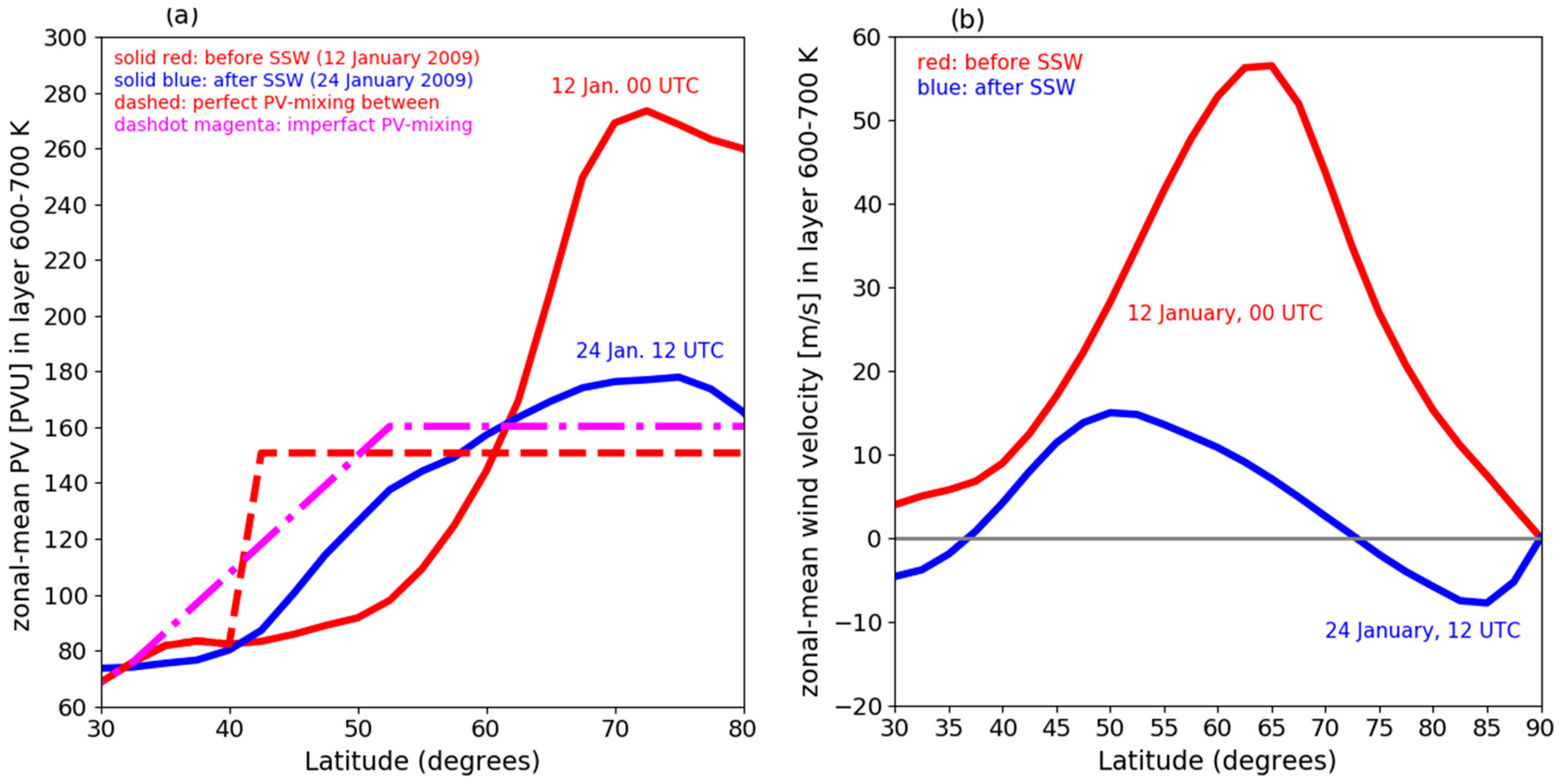
Figure 1a shows zonal-mean PV in the Northern Hemisphere in the isentropic layer between θ = 600 K and θ = 700 K (near p = 20 hPa), just before and just after the SSW of January 2009. This layer intersects the lower part of the upper stratospheric positive PV-anomaly over the Polar cap, as we shall see in Section 5. At these levels, the SSW started on 20 January 2009. During the SSW, high-PV air from higher latitudes is exchanged with low-PV air from lower latitudes. The effect of this exchange is manifest as the near destruction of the Polar cap positive PV-anomaly between 60° and 90° N and a simultaneous increase of zonal-mean PV at lower latitudes. This PV-exchange is not perfect. Nevertheless, we clearly observe (Figure 1a) a reduction of the zonal-mean meridional PV-gradient in the center of the “mixing zone”, as expected when turbulence mixes a materially conserved quantity like PV. A sharpening of the zonal-mean meridional PV-gradient is also observed at the edge of the mixing zone, between 40° N and 50° N, but not as strong as expected in the singular case of “perfect PV-mixing” between 40° N and the North Pole (dashed red line in Figure 1a). A piecewise linear PV-profile approximates reality better (the dash-dotted magenta line in Figure 1a). This piecewise linear PV-profile might be the time-average result of several separate PV-mixing events.

Figure 1b shows the layer-average zonal-mean zonal wind velocity in the layer between θ = 600 K and θ = 700 K for the same two dates, before and after the SSW of January 2009. An intense polar vortex, centered over the North Pole, exists before the SSW. The maximum zonal-mean circumpolar wind velocity (48 m s⁻¹) is observed at about 60° N. This feature is referred to as the polar night jet. During the SSW, the polar night jet vanishes, and westward circumpolar flow appears over the Polar cap. This zonal-mean zonal wind reversal is unexpected if, indeed, the SSW represents a case of near complete PV-mixing. The result of complete PV-mixing is a homogeneous PV-distribution in the PV-mixing zone, which, intuitively, should be associated with complete cessation or damping of the eastward winds in the mixing zone. So, the question is, why is there a reversal of the zonal-mean zonal wind within the mixing zone over the Polar Cap? This paper provides an answer to this question.

3. Zonal-Mean Balance

To understand the relation between the zonal-mean PV-distribution and the zonal-mean zonal wind velocity, PV-inversion is applied to the zonal-mean state of the atmosphere on the sphere. PV-inversion assumes that the zonal-mean circumpolar flow is in balance. By “balance” we mean hydrostatic balance and gradient wind balance. Hydrostatic balance in the isentropic coordinate system is expressed as

$${\displaystyle \frac{\mathsf{\partial }\Psi }{\mathsf{\partial }\theta }}=\Pi .$$

(2)

Here, $\Psi$ is the “isentropic stream function”, also known as the “Montgomery stream function” [17], defined as $\Psi \equiv gz+c_{p}T$, where z is the height above sea level of the isentropic surface and $g$ is the acceleration due to gravity (assumed constant). The Exner function, $\Pi$, is defined as

$$\Pi \equiv {\displaystyle \frac{c_{p}T}{\theta }}.$$

(3)

Gradient wind balance of the circumpolar flow in isentropic coordinates is expressed as [18],

$${\displaystyle \frac{u^{2}tan\varphi }{a}}+fu=-{\displaystyle \frac{\mathsf{\partial }\Psi }{\mathsf{\partial }y }}.$$

(4)

Here, y is the meridional coordinate (northward is positive), $\varphi$ is latitude, $a$ is the radius of the Earth (assumed constant), $u$ is zonal wind velocity, and $f$ is the Coriolis parameter ($f=2\Omega sin\varphi$, with $\Omega$ as Earth’s angular velocity). The derivative with respect to y is performed at constant θ.

This section demonstrates that the the stratosphere is in close zonal-mean gradient wind balance. The zonal-mean of any variable is indicated by square brackets. In the case of the zonal velocity, u, we have

$$\left[u\right]\equiv {\displaystyle \frac{1}{2\pi }}{\int }_0^{2\pi }ud\lambda .$$

(5)

Any variable is expressed as a sum of the zonal-mean value and a perturbation, indicated by an asterisk, e.g.,

$$u\equiv \left[u\right]+u^{*}.$$

(6)

Substituting this assumption into Equation (4) and taking the zonal-mean of the resulting equation yields,

$${\left[u_{gr}\right]}^2+{\displaystyle \frac{fa}{tan\varphi }}\left[u_{gr}\right]+{\displaystyle \frac{a}{tan\varphi }}{\displaystyle \frac{\mathsf{\partial }[\Psi ]}{\mathsf{\partial }y}}=0,$$

(7)

provided $\left[u^{*}{u}^{*}\right]\ll {\left[u\right]}^2$. The subscript “$gr$” stands for “gradient” wind. An explicit expression for the zonal-mean gradient wind is:

$$\left[u_{gr}\right]={\displaystyle \frac{fa}{2tan\varphi }}\left(-1\pm \sqrt{1-{\displaystyle \frac{4tan\varphi }{f^{2}a}}{\displaystyle \frac{\mathsf{\partial }[\Psi ]}{\mathsf{\partial }y}}}\right).$$

(8)

The gradient wind is calculated from Equation (8), using gridded reanalysis data of the isentropic stream function.

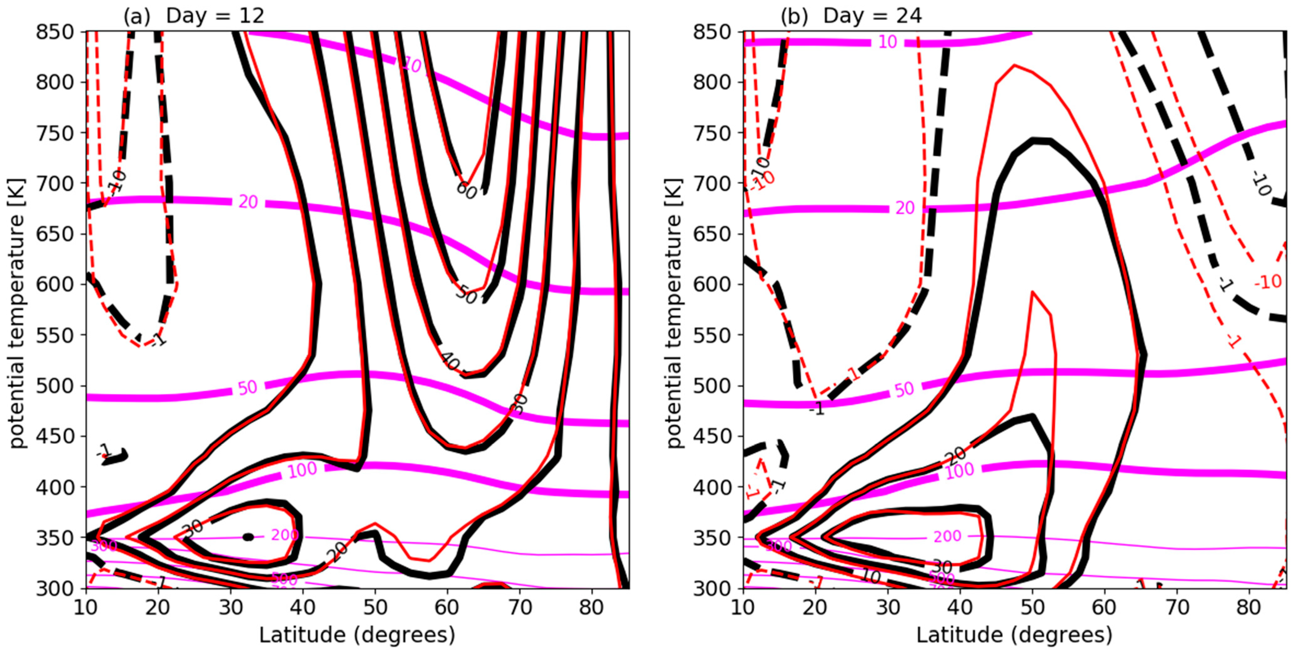
Figure 2 shows $\left[u_{gr}\right]$ as a function of latitude and potential temperature for the two dates, also highlighted in Figure 1. Also shown is $\left[u\right]$, according to the same reanalysis. Clearly, the SSW is associated with a spectacular change in the zonal-mean zonal wind in the mid- and high-latitude stratosphere. The polar night stratospheric cyclonic vortex above 400 K, including the intense polar night jet at 60° N, disappears and is replaced by a weaker anti-cyclonic vortex over the Polar cap. Meanwhile, the subtropical jet at 350 K is hardly affected.

Before the SSW, on 12 January 2009 (Figure 2a), $\left[u\right]$ and $\left[u_{gr}\right]$ are very similar, i.e., the atmosphere is in very close zonal-mean thermal wind balance. After the SSW, on 24 January 2009 (Figure 2b), this is also the case at most levels and latitudes equatorward of 40° N, while the actual wind and the gradient wind are somewhat less similar closer to the North Pole in the stratosphere. This may indicate that zonal-mean gradient wind balance has not yet been reached and/or that the condition, $\left[u^{*}{u}^{*}\right]\ll {\left[u\right]}^2$, is not well satisfied at very high latitudes.

Zonal-mean isentropic pressure, also shown in Figure 2, changes in accord with the balance requirements, as we shall see later. Before the SSW, on 12 January (Figure 2a), the isobaric surfaces in the stratosphere dip downwards over the Pole. After the SSW, on 24 January (Figure 2b), these same isobars bulge upwards over the Pole. This reflects isentropic mass flux convergence aloft over the Polar Cap and is a manifestation of the isobaric warming, which gives the event its name (SSW).

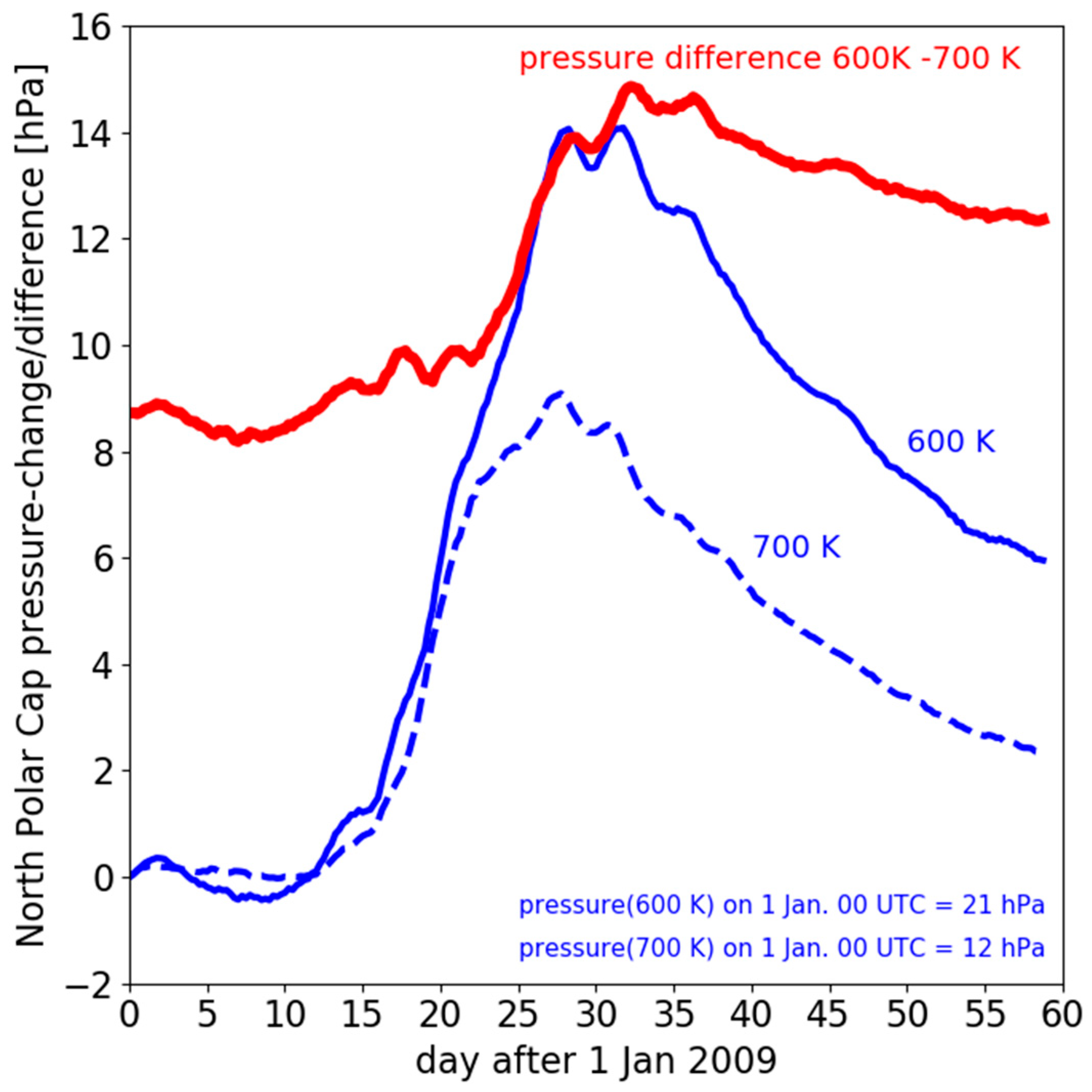
Figure 3 shows the area-mean isentropic pressure for θ = 600 K and for θ = 700 K over the North Polar cap, defined as the area for which $\varphi$ > 60° N, relative to the pressure on 1 January 2009 (00 UTC), as a function of time between 1 January and 28 February 2009. Pressure at 700 K over the North Polar cap increases by about 9 hPa between 15 January and 25 January. This is due to isentropic mass flux convergence at levels above 700 K. Somewhat lower, at 600 K, pressure over the North Polar cap increases by about 14 hPa between 15 January and 25 January. Therefore, the change in the pressure difference across the layer between 600 K and 700 K is 5 hPa between these dates. This measure of isentropic mass flux convergence over the North Polar cap in the layer between 600 K and 700 K is plotted also in Figure 3 (the red curve). Assuming hydrostatic balance, a change of the pressure difference of 5 hPa across a layer in the atmosphere is equivalent to an average increase of the mass in this layer of more than 50 kg m⁻², equivalent to more than a 50% increase in 10 days.

After the SSW, stratospheric temperatures over the North Polar cap are well above radiative equilibrium. Return to radiative equilibrium by net emission of long wave radiation is manifest as cross-isentropic downwelling and a decrease of isentropic pressure at all isentropic levels over the Polar cap. This pressure decrease is exponential in time. It is observed throughout the full month of February 2009 (Figure 3). The associated e-folding time decreases with height, being about 32 days at 600 K and about 23 days at the higher level of 700 K.

4. The PV-Inversion Equation

Can these large changes of the Polar Cap isentropic pressure be attributed to PV-mixing? A numerical experiment employing PV-inversion yields an answer to this question. This section sets the stage for this experiment. It derives the PV-inversion equation, the solution of which yields the balanced zonal-mean zonal wind velocity and the associated isentropic pressure distribution, given the zonal-mean PV-distribution.

The definition of zonal-mean potential vorticity, [Z], is,

$$\left[Z\right]=\left[{\displaystyle \frac{\zeta +f}{\sigma }}\right]\cong {\displaystyle \frac{\left[\zeta \right]+f}{\left[\sigma \right]}}.$$

(9)

The zonal-mean relative vorticity ($\left[\zeta \right]$) is defined as

$$\left[\zeta \right]={\displaystyle \frac{\left[u\right]tan\varphi }{a}}-{\displaystyle \frac{\mathsf{\partial }\left[u\right]}{\mathsf{\partial }y}}.$$

(10)

The zonal mean mass “density” in (x,y,θ) space ($\left[\sigma \right]$), henceforth referred as isentropic density, is defined as

$$\left[\sigma \right]=-{\displaystyle \frac{1}{g}}{\displaystyle \frac{\mathsf{\partial }\left[p\right]}{\mathsf{\partial }\theta }}.$$

(11)

Differentiating Equation (9) with respect to y and using Equation (11) yields (approximately),

$$\left[\sigma \right]{\displaystyle \frac{\mathsf{\partial }\left[Z\right]}{\mathsf{\partial }y}}={\displaystyle \frac{\mathsf{\partial }\left[\zeta \right]}{\mathsf{\partial }y}}+{\displaystyle \frac{\left[Z\right]}{g}}{\displaystyle \frac{\mathsf{\partial }}{\mathsf{\partial }\theta }}\left({\displaystyle \frac{\mathsf{\partial }\left[p\right]}{\mathsf{\partial }y}}\right)+\beta .$$

(12)

Here, $\beta \equiv {\displaystyle \frac{df}{dy}}$. Taking the zonal-mean of the hydrostatic balance equation (Equation (2)) combined with zonal-mean gradient wind balance equation (Equation (7)) yields the following equation for zonal-mean thermal wind balance:

$$f_{loc}{\displaystyle \frac{\mathsf{\partial }\left[u\right]}{\mathsf{\partial }\theta }}=-{\displaystyle \frac{\mathsf{\partial }\left[\Pi \right]}{\mathsf{\partial }y}},$$

(13)

with

$$f_{loc}\equiv f+{\displaystyle \frac{2\left[u\right]tan\varphi }{a}}.$$

(14)

The definition of the Exner function (Equation (3)), combined with Equation (1), gives

$$\Pi \equiv T{\left({\displaystyle \frac{p}{p_{ref}}}\right)}^{\kappa },$$

(15)

Using Equation (15) and the ideal gas law ($p=R\varrho T$, $\varrho$ being density), the right-hand side of Equation (13) can be expressed as

$${\displaystyle \frac{\mathsf{\partial }\left[\Pi \right]}{\mathsf{\partial }y}}\approx {\displaystyle \frac{1}{\theta \left[\varrho \right]}}{\displaystyle \frac{\mathsf{\partial }\left[p\right]}{\mathsf{\partial }y}},$$

(16)

so that Equation (13) becomes,

$$f_{loc}\theta \left[\varrho \right]{\displaystyle \frac{\mathsf{\partial }\left[u\right]}{\mathsf{\partial }\theta }}=-{\displaystyle \frac{\mathsf{\partial }\left[p\right]}{\mathsf{\partial }y}}.$$

(17)

Using Equations (10) and (17) to eliminate vorticity and pressure in Equation (12), this equation becomes,

$${\displaystyle \frac{\mathsf{\partial }}{\mathsf{\partial }y}}\left({\displaystyle \frac{\mathsf{\partial }\left[u\right]}{\mathsf{\partial }y}}-{\displaystyle \frac{\left[u\right]tan\varphi }{a}}\right)+{\displaystyle \frac{\left[Z\right]}{g}}{\displaystyle \frac{\mathsf{\partial }}{\mathsf{\partial }\theta }}\left(f_{loc}\theta \left[\varrho \right]{\displaystyle \frac{\mathsf{\partial }\left[u\right]}{\mathsf{\partial }\theta }}\right)=\beta -\left[\sigma \right]{\displaystyle \frac{\mathsf{\partial }\left[Z\right]}{\mathsf{\partial }y}}.$$

(18)

Equation (18) is an elliptic partial differential equation, known as the “PV-inversion equation”. It is an expression of zonal-mean thermal wind balance in terms of zonal-mean potential vorticity, $\left[Z\right]$, and zonal-mean zonal wind velocity, $\left[u\right]$. Equation (18) was derived and solved numerically first by Hinssen et al. [19]. Equation (18) for a balanced vortex on an “f-plane”, i.e., with β = 0, was derived earlier by Hoskins et al. [20] (eq. 29, page 901) and solved by Thorpe [21].

The idea is that the circumpolar velocity field ([u]), associated with an axisymmetric vortex centered over the Pole on the spherical Earth, is induced by the PV-field. In other words, for a prescribed zonal-mean PV-field, Equation (18) is solved (inverted) to yield the zonal-mean zonal wind that is associated with this PV-field in a balanced atmosphere.

5. Solution of the PV-Inversion Equation for the January-Mean PV-Distribution

The zonal mean potential vorticity, $\left[Z\right]$, is partitioned into a part, $Z_{ref}$, which is associated with a reference state, and a part, $Z\prime$, which is associated with the zonal-mean “PV-anomaly”, as follows.

$$\left[Z\right]=Z_{ref}+Z^{\prime }.$$

(19)

If the reference state is defined such that the right-hand side of Equation (18) is equal to zero, i.e.,

$$\beta -{\sigma }_{ref}{\displaystyle \frac{\mathsf{\partial }{Z}_{ref}}{\mathsf{\partial }y}}=0,$$

(20)

where ${\sigma }_{ref}$ is the isentropic density in the reference state, defined as the area-weighted average of the isentropic density, i.e.,

$${\sigma }_{ref}={\displaystyle \frac{\int \left[\sigma \right]cos\varphi d\varphi }{\int cos\varphi d\varphi }},$$

(21)

Then, under not very restrictive circumstances, the reference state is associated with the state of rest ([u] = 0), as is explained below Equation (22). Equations (20) and (21) together imply that the reference isentropic potential vorticity is given by

$$Z_{ref}={\displaystyle \frac{f}{{\sigma }_{ref}}}.$$

(22)

Because f depends on y, and ${\sigma }_{ref}$ depends on θ, $Z_{ref}$ depends both on θ and y. If $\left[\sigma \right]={\sigma }_{ref}$ and $\left[Z\right]=Z_{ref}$, then $\left[\zeta \right]=0$. If $\left[Z\right]=Z_{ref}$, and thus $Z^{\prime }=0$ (no “PV-anomalies”), the “forcing term” on the r.h.s. of Equation (18) is equal to zero. The solution of Equation (18) for $\left[Z\right]=Z_{ref}$ with [u] = 0 at the boundaries of the domain of interest, is [u] = 0 everywhere inside this domain. Here, the boundaries of the domain of interest are the North Pole, a low-latitude parallel, the Earth’s surface, and a high-level isentropic surface. In summary, therefore, the reference state is defined such that it corresponds to the state of rest of the atmosphere with respect to the rotating Earth.

The PV-anomaly is associated with, or “induces”, the full wind field. In this context, it might be better to refer to the “positive and negative anomalies” of $Z$ as the “maxima and minima” of $Z^{\prime }$. We will stick to the former terminology because this terminology is commonly used.

The PV-anomaly, $Z^{\prime }$, is related in a specific way to the separate vorticity- and isentropic density anomalies. Using the binomial approximation, this relation is given by,

$${\displaystyle \frac{Z^{\prime }}{Z_{ref}}}\cong {\displaystyle \frac{{\zeta }^{\prime }}{f}}-\left(1+{\displaystyle \frac{{\zeta }^{\prime }}{f}}\right){\displaystyle \frac{{\sigma }^{\prime }}{{\sigma }_{ref}}},$$

(23a)

provided that $\left|{\displaystyle \frac{{\sigma }^{\prime }}{{\sigma }_{ref}}}\right|<<1$. In non-dimensional form Equation (23a) is

$$Z^{+}\cong {\zeta }^{+}-\left(1+{\zeta }^{+}\right){\sigma }^{+},$$

(23b)

in which the normalized anomalies are defined as,

$$Z^{+}\equiv {\displaystyle \frac{Z^{\prime }}{Z_{ref}}}; {\zeta }^{+}\equiv {\displaystyle \frac{{\zeta }^{\prime }}{f}}; {\sigma }^{+}\equiv {\displaystyle \frac{{\sigma }^{\prime }}{{\sigma }_{ref}}}.$$

(24)

If ${\zeta }^{+}\ll 1$, Equation (23b) becomes,

$$Z^{+}\cong {\zeta }^{+}-{\sigma }^{+}.$$

(25)

The partitioning of $Z^{+}$ between the magnitudes of ${\zeta }^{+}$ and ${\sigma }^{+}$ is determined from the solution of the PV-inversion equation (Equation (18)). Ernst Kleinschmidt [20,22] was the first, in the 1950s, to formulate the following general rules about this partitioning. A PV-anomaly ($Z^{+}\ne 0$) in a balanced atmosphere cannot appear exclusively as a vorticity anomaly. In other words, ${\zeta }^{\prime }\ne 0$, while ${\sigma }^{+}=0$, is impossible. Neither can a PV-anomaly in a balanced atmosphere appear exclusively as an isentropic density anomaly. In other words, ${\sigma }^{\prime }\ne 0$, while ${\zeta }^{+}=0$, is impossible.

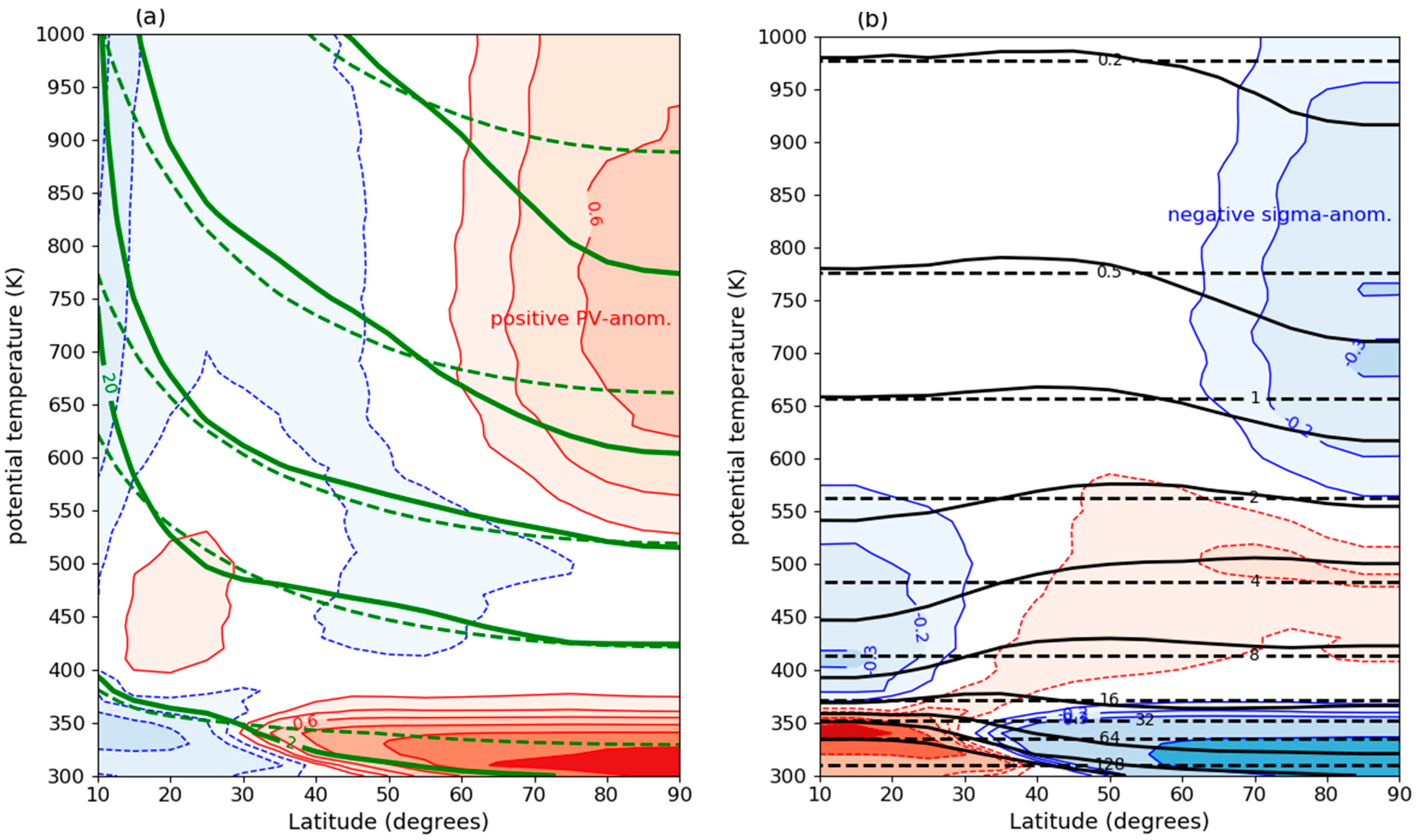
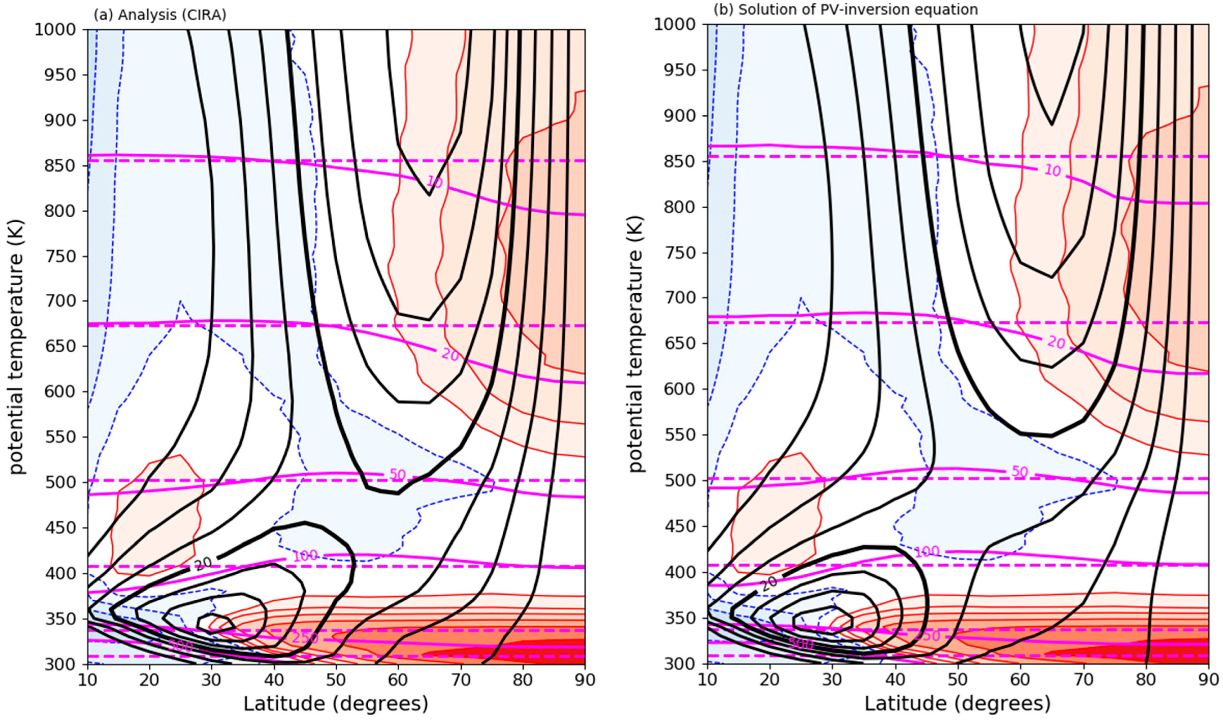
Figure 4 shows $Z^{+}$(panel a) and ${\sigma }^{+}$ (panel b) in January in the Northern Hemisphere in the COSPAR International Reference Atmosphere [23] as a function of potential temperature and latitude. Positive values of $Z^{+}$ are shaded in red in panel (a) (Figure 4a). These regions correspond to negative values of ${\sigma }^{+}$, shaded in blue in panel (b) (Figure 4b). This is an expression of Kleinschmidt’s second principle [3], which states that “within an isolated air mass with abnormal potential vorticity, in thermal wind balance, the isentropic density deviates from the normal in the opposite sense as the potential vorticity”. In other words, in an atmosphere in thermal wind balance, positive values of $Z^{+}$ are associated with negative values of ${\sigma }^{+}$, as is nicely illustrated by Figure 4.

Two positive PV-anomalies ($Z^{+}>0)$, centered over the North Pole, can easily be distinguished in Figure 4a. First, a Polar cap stratospheric PV-anomaly above 550 K extending from the North Pole to about 60° N and, second, a PV-anomaly coinciding with the lowermost stratosphere, extending from the North Pole to about 30° N. The first PV-anomaly induces the polar night stratospheric jet, while the second PV-anomaly induces the subtropical jet [19].

In the layer between these two positive PV-anomalies, we observe a reduced meridional slope of $\left[Z\right]$-isopleths. This is a typical consequence of meridional PV-mixing, leading to the formation of an atmospheric “surf zone” [24], which is characterized by a positive PV-anomaly equatorward of a negative PV-anomaly, as is indeed observed in the between θ = 400 K and θ = 550 K.

The zonal-mean PV-distribution is determined by the following processes.

(1)

Cross-isentropic down- or upwelling due to radiative flux divergence.

(2)

Isentropic meridional PV-mixing due to breaking planetary waves.

(3)

Adjustment to thermal wind balance by a secondary zonally symmetric meridional overturning circulation, which is referred as the Ferrel cell.

This paper intends to present evidence of the idea that the erosion or elimination of the radiatively induced (process 1) stratospheric Polar cap positive PV-anomaly by PV-mixing (process 2), in an atmosphere that tends to adjust continuously to zonal-mean thermal wind balance (process 3), should be concomitant with the weakening or elimination of the associated negative isentropic density anomaly by poleward isentropic mass flux convergence. This idea is tested here by employing PV-inversion.

Kleinschmidt’s first principle, derived from PV-inversion [3], states that “within an isolated air mass with abnormal potential vorticity, in thermal wind balance, the absolute vorticity deviates from the normal in the same sense as the potential vorticity”. The “normal” is identified with the state of rest, i.e., with $Z=Z_{ref}$ and $\left[u\right]=0$. Kleinschmidt’s first principle is illustrated in Figure 5a. The upper stratospheric positive PV-anomaly induces the cyclonic circumpolar polar night jet, while the positive PV-anomaly in the lowermost stratosphere induces the cyclonic circumpolar subtropical jet. Isobaric surfaces are depressed within and below the Polar cap upper stratospheric PV-anomaly, indicating that, at least down to 100 hPa, the Polar cap is relatively cold due to the presence of this positive stratospheric PV-anomaly aloft. The upward influence of the lowermost stratospheric PV-anomaly, which tends to raise the isobars above it, is clear at latitudes in the range, 30°–60° N, outside the region of the downward influence of the stratospheric PV-anomaly (60°–90° N). The 100 hPa and 50 hPa isobars indeed bend upwards between 30° N and 60° N. The relatively warm conditions at these pressure-levels and latitudes can, therefore, be attributed to the presence of the lowermost stratospheric PV-anomaly. Further equatorward, we again observe a downward bending of the 100 hPa and 50 hPa isobars. This can be attributed to the reverse PV-distribution in the subtropics, with a positive PV-anomaly centered at 450 K above a negative PV-anomaly centered at 350 K.

Figure 5b shows the $\left[u\right]$- and $\left[p\right]$-distributions, according to the solution of the PV-inversion Equation (18), given the CIRA zonal-mean PV- ($\left[Z\right]$-) distribution and realistic boundary conditions. The boundaries of the domain of this numerical solution of Equation (18) are the Earth’s surface (lower boundary), the 2250 K isentropic surface (upper boundary), and the North Pole and 10° N-parallel (side boundaries). For technical details of the numerical method of solution of Equation (18), see [16]. The striking similarity of the numerical solution of Equation (18) (Figure 5b), to the analysis of observations (Figure 5a), proves that the time-average atmosphere is in close zonal-mean thermal wind balance, as is suggested also by Figure 2.

6. Inverting PV After Perfect PV-Mixing Poleward of a Fixed Latitude

To better understand the influence of isentropic PV-mixing by eddies on the zonal-mean state of the atmosphere, we perform a simple numerical thought experiment, employing PV-inversion. The experiment begins by assuming that the atmosphere is in the average winter state shown in Figure 4 and Figure 5a. Next, we imagine that PV is mixed perfectly on isentropic surfaces. This occurs in a latitude-band between the latitudes ${\varphi }_S$ and ${\varphi }_N$. Perfect isentropic PV-mixing will lead to a latitude-independent isentropic PV-distribution in the mixing zone, i.e., a state in which $Z\left(y,\theta \right)=Z_0\left(\theta \right)$ between the latitudes ${\varphi }_S$ and ${\varphi }_N$. Because PV-mixing along isentropic surfaces is performed under the constraint of material conservation of PV, we find $Z_0$ from

$$Z_0\left(\theta \right)={\displaystyle \frac{{\int }_{{\varphi }_S}^{{\varphi }_N}Z\left(\varphi ,\theta \right)cos\varphi d\varphi }{{\int }_{{\varphi }_S}^{{\varphi }_N}cos\varphi d\varphi }}.$$

(26)

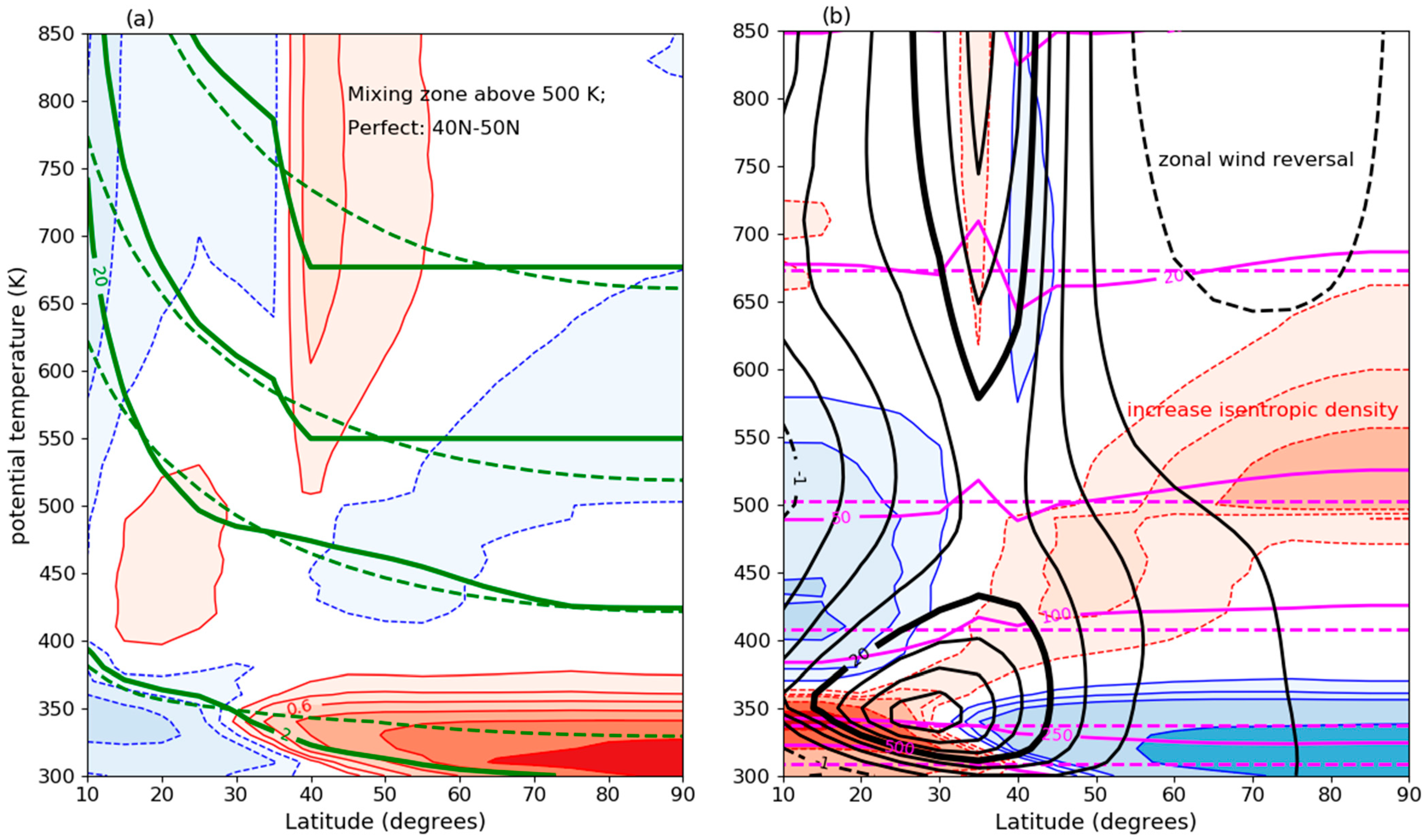
Zonal-mean PV-anomalies will appear after the hypothetical PV-mixing. This is illustrated in Figure 6a. In this example, PV between ${\varphi }_S$ = 40° N and ${\varphi }_N$ = 90° N is mixed completely while conserving PV. The ideal planetary wave-breaking surf zone, therefore, consists of a large interior region with constant [Z], centered over the Pole, and bordered on the equatorward side by a “potential vorticity step” or “PV-step” [25]. Because of the latitude-dependence of $Z_{ref}$, a negative PV-anomaly poleward of a positive PV-anomaly appears due to PV-mixing. If the atmosphere in our experiment adjusts to thermal wind balance after the PV-mixing, the zonal-mean zonal wind, [u], will change non-trivially. The new distribution of [u] can be deduced from the PV-inversion of the new PV-distribution (the solution of Equation (18)).

Figure 6b shows the fields of zonal-mean zonal wind, zonal-mean pressure zonal-mean isentropic density resulting from PV-inversion of the zonal-mean PV-field after complete PV-mixing between 40° N and the North Pole above 500 K (Figure 6a) of the observed January-mean zonal-mean PV-distribution (Figure 5a). As expected, the negative PV-anomaly in the interior of the surf zone, which encompasses the Polar Cap in this example, induces a westward (anticyclonic) zonal-mean zonal wind ([u] < 0) between 60° N and the North Pole. The positive PV-anomaly on the equatorward side of the surf zone induces an eastward zonal-mean zonal wind ([u] > 0). The zonal-mean zonal wind is both locally weakened and locally intensified by a mere homogenization of potential vorticity on isentropic surfaces due to turbulent mixing on the rotating spherical Earth.

By comparing the zonal-mean isentropic density field before (Figure 4b) and after (Figure 6b) the perfect PV-mixing above 500 K, we conclude that PV-mixing is indeed associated with a poleward shift of mass within the mixing zone, as expected. The negative isentropic density anomaly over the Polar cap (blue shading in Figure 4b) vanishes (red shading or no shading in Figure 6b). The implied poleward mass flux in the mixing zone is revealed by a spectacular rise of the isobars over the Polar cap. The isobaric temperature rise over the Polar cap is about 40 K at 50 hPa! This warming is a direct consequence of the poleward shift of mass required to maintain zonal-mean thermal wind balance and is very comparable to the observed Polar cap warming during the SSW of January 2009. Note that Polar cap warming occurs also below the PV-mixing zone, for example, at 100 hPa (Figure 6b).

On the equatorward side of the ideal PV-mixing zone, mass is shifted equatorward. This is because of the appearance of a PV-step at the edge of the ideal PV-mixing zone, with $Z^{+}<0$ on its equatorward side and $Z^{+}>0$ on its poleward side. An eastward jet is induced by this PV-step with cyclonic relative vorticity on its poleward side and anticyclonic relative vorticity on its equatorward side. The formation of such an eastward jet at low latitudes is probably never observed in the real world. This is because PV-mixing is never manifest as a singular event of perfect mixing between fixed latitudes. We must, therefore, view the case of perfect PV-mixing, studied here, as an ideal example of PV-mixing. This example guides our understanding of the general consequences of PV-mixing for the mass-distribution in the atmosphere.

7. Discussion and Conclusions

This paper points to the direction we need to look in to understand the mechanism that causes the poleward transfer of mass in the stratosphere, i.e., the poleward component of the Brewer–Dobson circulation. This mass transfer is a likely reflection of the almost continuous breakdown of the positive Polar cap PV-anomaly by PV-mixing, while the atmosphere maintains zonal-mean thermal wind balance.

The effect of isentropic PV-mixing on the mass distribution in the atmosphere cannot usually be isolated from the effect of cross-isentropic mass fluxes on the mass distribution. This is because both processes occur continuously and simultaneously. In the stratosphere, however, isentropic PV-mixing is a highly intermittent process that occurs in the winter, mostly as relatively isolated and very intense Sudden Stratospheric Warming (SSW) events.

Due to its abruptness, a major SSW is a very good example of isentropic PV-mixing, although, even in this case, isentropic PV-mixing is not perfect, in part due to the very large scale of the planetary waves. For example, in Figure 1a, we observe a slight reversal of the meridional PV-gradient over the Polar cap. This is a typical manifestation of mixing by eddies with spatial scales comparable to the spatial scale of the mixing zone itself [14]. Nevertheless, we observe the typical dynamical consequences of PV-mixing on the spherical Earth while the atmosphere maintains zonal-mean thermal wind balance, such as the reversal of [u] over the Polar cap. It should be remarked that the strength of the reversal of [u] is very sensitive to the latitude of the equatorward edge of the PV-mixing zone. In other words, a smaller (larger) value of ${\varphi }_S$, than the value chosen here (40°), leads to a significant strengthening (weakening) of the reversal of [u].

Kleinschmidt’s third principle, derived from PV-inversion, states that a cold air mass in thermal wind balance only remains cold as long as there are masses of high potential vorticity above it. When this condition is no longer fulfilled, the air sinks down and loses the character of a cold air mass. Exactly this happens during an SSW. The atmosphere over the North Polar cap in both the lower stratosphere and the troposphere is cold because of the presence of a positive PV-anomaly aloft. During a major SSW, isentropic PV-mixing eliminates the stratospheric positive PV-anomaly, and with it, the negative isentropic density anomaly, while zonal-mean thermal wind balance is approximately maintained. In accord with Kleinschmidt’s third principle, the Polar air mass below the level of PV-mixing loses its character of a cold air mass. This can only be the consequence of a poleward isentropic mass flux at the level of the positive PV-anomaly before being eliminated by mixing.

In summary, this paper shows that the poleward mass flux in the stratosphere is a manifestation of the adjustment of the atmosphere to zonal-mean thermal wind balance while potential vorticity is mixed irreversibly by large-scale atmospheric turbulence. This explanation does not rely on the existence in the stratosphere of a westward drag on the eastward flow by planetary waves or eddies.

Some questions remain. For instance, how are Kleinschmidt’s first two principles (Section 5) satisfied after the positive Polar cap PV-anomaly has been eliminated by PV-mixing? In other words, how does the atmosphere transfer mass toward the North pole while also transferring vorticity in the opposite direction to maintain zonal-mean thermal wind balance? Because isentropic surfaces are impermeable to vorticity [26], vorticity-transfer is restricted to isentropic surfaces. But if the adjustment is adiabatic mass-transfer occurs along isentropic surfaces also. This question will be addressed in a future paper.