Article

Improving the Prediction of Land Surface Temperature Using Hyperparameter-Tuned Machine Learning Algorithms

1
Department of Civil Engineering, Indian Institute of Technology (BHU), Varanasi 221005, India
2
Department of Building, Energy and Material Technology, UiT, The Arctic University of Norway, 8515 Narvik, Norway
*
Author to whom correspondence should be addressed.
Atmosphere 2025, 16(11), 1295; https://doi.org/10.3390/atmos16111295
Submission received: 29 September 2025 / Revised: 5 November 2025 / Accepted: 7 November 2025 / Published: 15 November 2025
(This article belongs to the Special Issue UHI Analysis and Evaluation with Remote Sensing Data (2nd Edition))

Abstract

Land surface temperature (LST) is a critical variable for understanding energy exchanges and water balance at the Earth’s surface, as well as for calculating turbulent heat flux and long-wave radiation at the surface–atmosphere interface. Remote sensing techniques, particularly using satellite platforms like Landsat 8 OLI/TIRS and Sentinel-2A, have facilitated detailed LST mapping. Sentinel-2 offers high spatial and temporal resolution multispectral data, but it lacks thermal infrared bands, which Landsat 8 can provide a 30 m resolution with less frequent revisits compared to Sentinel-2. This study employs Sentinel-2 spectral indices as independent variables and Landsat 8-derived LST data as the target variable within a machine-learning framework, enabling LST prediction at a 10 m resolution. This method applies grid search-based hyperparameter-tuned machine learning algorithms—Random Forest (RF), Gradient Boosting Machine (GBM), Support Vector Machine (SVM), and k-Nearest Neighbours (kNN)—to model complex nonlinear relationships between the spectral indices (NDVI, NDWI, NDBI, and BSI) and LST. Grid search, combined with cross-validation, enhanced the model’s prediction accuracy for both pre- and post-monsoon seasons. This approach surpasses earlier methods that either employed untuned models or failed to integrate Sentinel-2 data. This study demonstrates that capturing urban thermal dynamics at fine spatial and temporal scales, combined with tuned machine learning models, can enhance the capability of urban heat island monitoring, climate adaptation planning, and sustainable environmental management models.

1. Introduction

Land surface temperature (LST) is defined as turbulent heat flow and long-wave radiation exchange at the surface–atmosphere interface, and many strategies exist to obtain LST data from space using satellite imagery [1]. LST directly displays the fluctuations that occur in the response of vegetation and bare soil to solar irradiance. These fluctuations are due to various factors, including cloud cover, atmospheric aerosol concentrations, and the diurnal solar cycle. LST is a key parameter for studying the physical processes of energy at the surface and in water balance [2]. It is used in applications such as weather predictions, climate modelling, agriculture, and urban heating effects [2,3,4,5,6,7,8,9,10].
The advent of remote sensing technologies, such as Landsat 8’s Operational Land Imager/Thermal Infrared Sensor (OLI/TIRS) and Sentinel-2A, has significantly enhanced our understanding of land processes [11,12]. Landsat 8 provides global coverage for long-term monitoring and has thermal infrared (TIR) sensors. While Sentinel 2A does not have TIR sensors, it offers higher spatial and temporal resolution than Landsat, enabling it to produce more detailed maps of the observed area.
This study proposes a methodology to use the spectral bands of Sentinel-2 (S2) to predict LST. Sentinel-2A provides multispectral imagery (10 m) with a revisit frequency of every five days. The lack of thermal bands can be overcome by integrating Landsat 8/9 with S2 Multispectral data. The revisit time can also be reduced from 15 days to three days, allowing for continuous land cover monitoring and the creation of medium-resolution data products. Landsat 8/9 LST is downscaled to a 10 m spatial resolution by integrating with Sentinel-2 data. Previous fusion methods, such as DisTrad, TsHARP, and STARFM (Spatial and Temporal Adaptive Reflectance Fusion Model), have achieved finer-scale LST estimation by combining coarse and fine imagery [13]. These approaches, such as ESTARFM, blend data from sensors like MODIS and Landsat to create high-frequency, high-resolution thermal maps [13,14]. However, they rely on linear assumptions or fixed weighting schemes, which limit their adaptability to complex urban environments [14].
The integration of other satellite data has been investigated in some studies; for example, S2 data were used to reduce MODIS data from a 1000 m resolution to 10 m [8]. MODIS offers daily worldwide coverage; its application in cities with fine-scale, variable land cover is limited by its large cell size. Therefore, the coarse-scale MODIS data is not suitable for capturing the acceptable temperature variations found in dense cities; thus, downscaled estimates are unable to represent actual high-resolution surface temperatures [15].
Four spectral indices were selected—NDVI, NDWI, NDBI, and BSI—representing vegetation, moisture, built-up, and bare soil components, respectively. These indices collectively explain the major land surface characteristics that influence LST variability. The chosen combination effectively captures biophysical diversity and has been widely validated for LST modelling in prior studies.
To date, the prediction of LST using machine learning algorithms with Sentinel-2-derived indices has been underexplored in the literature, particularly with regard to hyperparameter tuning to optimise model performance in multi-seasonal and riverside urban regions. Recent studies have demonstrated the efficacy of machine learning models [16]. A study in Yazd, Iran, a typical arid region, utilised Gradient Boosting Machines (GBMs) to estimate LST with high accuracy, achieving RMSE values as low as 0.27–0.32 °C. [17]. Despite extensive data integration studies, hyperparameter-tuned machine learning models have not been utilised for Sentinel-2 data in the prediction of LST. This study fills this gap by applying hyperparameter-tuned Random Forest (RF), Gradient Boosting Machine (GBM), Support Vector Machine (SVM), and k-Nearest Neighbours (kNN) algorithms to predict LST using spectral indices derived from Sentinel-2 data, to improve the traditional 30 m Landsat LST estimates.
The parameters, such as tree counts and depth in RF and GBM, kernel and regularisation parameters in SVM, and neighbourhood size in kNN, were optimally tuned to reduce the prediction error. The methodological enhancement enabled the models to effectively capture complex, nonlinear relationships between the spectral indices (NDVI, NDWI, and NDBI) and LST variations, resulting in the higher accuracy that is essential for understanding urban heat dynamics for better environmental management.

2. Materials and Methods

2.1. Study Area

The study area is located on the left bank of the Ganges River in Varanasi district, Uttar Pradesh, India (Figure 1). The district is generally flat, with the Ganges River being the most crucial stream. The average land surface is between 85 and 105 m above mean sea level. During the summer months, the climate is hot and humid, with temperatures often exceeding 45 degrees Celsius. Summer is longer than winter, with temperatures dipping to 7 degrees Celsius. The monsoons bring torrential rains and the average annual rainfall in the area is 1019 mm.
The city is developing rapidly, and urbanisation has already contributed to the warming conditions, amplifying the thermal stresses experienced in the region due to both global and local warming factors [18]. The area’s location along the Ganges has significant hydrological relevance, as it links surface temperature variations with riverine and urban environmental processes, which are central to sustainable, climate-resilient city planning.
Studies have been published that used data from various satellite sensors to measure LST within cities, identifying heat islands and zones under thermal stress [19].

2.2. Data Acquisition and Preprocessing

It is essential for the city’s heterogeneous urban surfaces that consistent and transparent processing is ensured across multiple years. We used the Landsat 8 surface temperature product and Sentinel-2 surface reflectance images acquired on the same date whenever possible. In cases where imagery from both satellites was not available for the same day, we used datasets with the closest acquisition dates (≤1 day) to maintain comparable spectral conditions [20].
Both datasets were atmospherically corrected to surface reflectance using the Sen2Cor on Sentinel-2 [21].
LST (target) was derived from Landsat 8 TIRS Band 10 (~10.9 µm, 30 m resolution), while the predictor variables were obtained from Sentinel-2 MSI bands: B2 (0.490 µm, 10 m), B3 (0.560 µm, 10 m), B4 (0.665 µm, 10 m), B8 (0.842 µm, 10 m), and B11 (1.610 µm, 20 m).

2.3. Land Surface Temperature (LST) Calculation

In this study, we have utilised the Surface Temperature (ST) band available on Google Earth Engine, with the product ID LANDSAT/LC08/C02/T1_L2. The key temperature data, located in the ST_B10 field, is supplied in Kelvin units after appropriate scaling. The product is derived from the Thermal Infrared Sensor (TIRS) Band 10, using a single-channel atmospheric correction algorithm [12] that accounts for atmospheric effects, surface emissivity, and sensor calibration parameters. This dataset is valuable in hydrology, climate studies, and environmental management, enabling users to obtain temperature data at a spatial resolution of 30 m and a temporal frequency ranging from 16 days to monthly composites. The atmospheric correction algorithms and calibration methods are based on rigorous validation efforts, including research led by institutions such as the Rochester Institute of Technology (RIT) and the NASA Jet Propulsion Laboratory (NASA JPL). The scale and offset for Landsat Collection 2 Surface Temperature (ST) products are 0.00341802 and 149.0, respectively.

2.4. Spectral Indices

2.4.1. Normalised Difference Vegetation Index (NDVI)

The NDVI is crucial for distinguishing different land cover types, and for monitoring vegetation growth, detecting land use changes, assessing crop health, and estimating biomass. Its values range from −1.0 to +1.0 and have been shown to correlate strongly with thermal bands [22]. The NDVI is calculated per pixel by taking the normalised differences in the red band (0.64–0.67 μm) and the near-infrared band (0.85–0.88 μm)
N D V I = N I R R e d N I R + R e d

2.4.2. Normalised Difference Water Index (NDWI)

Water bodies strongly absorb radiation in the visible to infrared wavelength range, resulting in low reflectance. Thus, the NDWI is particularly effective for detecting water bodies. It is a crucial tool in fields such as hydrology, agriculture, and environmental monitoring, enabling the identification of water bodies, tracking changes in water levels, and assessing the health of vegetation [23]. NDWI values range from −1 to +1, where values approaching +1 indicate the existence of water, and those closer to −1 suggest its absence. Numerous studies have investigated the relationship between LST and the NDWI [24]. The index is derived using the NIR and green bands and is computed as follows:
N D W I =   G r e e n N I R G r e e n + N I R

2.4.3. Normalised Built-Up Index (NDBI)

Built-up areas exhibit different thermal properties compared to natural surfaces, thus impacting LST values [25]. The range of NDBI values varies from −1 to 1. An increased NDBI number indicates a higher percentage of built-up area. In comparison to the NIR wavelength range (0.76~0.90 μm), built-up areas have increased reflectance in the Mid-Infrared (MIR) wavelength range (1.55~1.75 μm) when compared to other land use/cover surfaces [25]. The NDBI helps map urban areas, and is expressed as
N D B I = S W I R 1 N I R S W I R 1 + N I R

2.4.4. Bare Soil Index (BSI)

The BSI is a spectral index that identifies and quantifies bare soil in satellite imagery. It helps differentiate between bare soil, vegetation, and built-up areas [26]. The BSI can be calculated using Equation (4) for S2 data, typically using reflectance values from satellite bands as follows:
B S I   =   ( R e d + S W I R )     ( N I R + B l u e ) ( R e d + S W I R )   +   ( N I R + B l u e )
The correlation between the BSI and LST generally indicates that areas with higher bare soil exposure exhibit higher surface temperatures [26]. This relationship is significant in understanding the effects of land use/land cover change (LUCC) on regional climates, particularly in urbanised and degraded environments [26].
A flow chart of the methodology used in this work is shown in Figure 2.

2.5. Machine Learning Algorithms

RF, GBM, SVM and kNN were used because they are strong, data-efficient learners for tabular predictors (spectral indices), capture nonlinear relations, are robust on moderate sample sizes, and remain interpretable and fast to tune. The models were implemented in R (R Studio version 4.2.2) using the following packages: randomForest v4.7-1.1 (RF), gbm v2.1.8 (GBM), e1071 v1.7-14 (SVM/SVR), and kknn v1.3.1 (kNN). We used identical splits for all models (RF, GBM, SVR, \nd kNN): 70/15/15% train/val/test, with a fixed seed of 42, and scene-wise blocking to ensure that a Landsat–Sentinel pair never spans across splits.
A 5-fold CV was run on the training set (same folds for all models), the validation set guided choices, and the test set was used once for results. Standardisation: Sentinel-2 index features were z-scored (train-fit, then applied to val/test) for SVR and kNN; RF/GBM used raw features. To avoid leakage after masking, missing values were removed within folds; the methodology for developing these models is described below.

2.5.1. Random Forest (RF)

The random forest model was developed using R Studio. It is a well-known supervised machine learning technique [27]. It comprises multiple decision trees, each constructed using some form of randomisation. The Random Forest algorithm predicts Y in two main steps: First, it builds numerous decision trees using random subsets of data and features. Then, it combines their results by averaging for regression or voting for classification to make the final prediction.
Training Stage: The algorithm creates an ensemble of decision trees for each tree i in the ensemble (where i = 1 to Ntrees) to produce precise forecasts. The training data’s subsets are selected randomly with replacement during the training process, and a subset of features is chosen for every decision tree. This randomness aids the tree’s diversity. After that, each tree is trained using these features and data, which enables the model to identify patterns successfully.
Prediction Stage: Each tree within the ensemble predicts Yi using its decision-making process when a fresh sample with feature value x is added. While the final judgement in classification is determined by collecting the majority vote from all the trees, the final prediction of a random forest in regression is obtained by averaging the predictions from each tree.
This ensemble approach leverages the collective insight of all trees, leading to a more robust and accurate prediction.
For regression
1 N t r e e s Y i   f o r   i = 1   t o   N t r e e s
It is determined by the majority vote among the predictions for classification.
Y = m a j o r i t y   v o t e ( Y 1 , Y 2 ,   . . .   , Y N t r e e s )
Ntrees represents the number of trees in the random forest, and m refers to the number of features randomly chosen for each tree.

2.5.2. Support Vector Regression (SVR)

SVR is a well-liked machine learning method for capturing and modelling nonlinearity in various applications [6]. SVR is an SVM extension that uses a hyperplane to divide input data into two classes. The closest data points to the hyperplane, or a set of support vectors, determine the hyperplane [28]. The new data point value is predicted using these support vectors to make predictions in the SVR model.
The equation for an SVM used in binary classification is
f ( x ) = s i g n ( w x + b )
where f(x) represents the decision function that forecasts the class of the incoming sample, the weight vector is x, and the bias term is b. The dot (.) represents the dot product between w and x. The sign function determines the predicted class label by comparing it to the sign of the decision function.
SVM aims to determine the optimal values of w and b that maximise the margin while accurately classifying the majority of samples. The samples nearest to the hyperplane are known as support vectors, and they play a crucial role in defining the decision boundary [28].

2.5.3. K-Nearest Neighbours (kNN)

The kNN algorithm is an effective technique used for regression and classification [29]. It classifies a new instance by comparing it to existing cases, assuming that the new instance is like the ones it closely resembles. The kNN algorithm is commonly known as a lazy learning algorithm due to its ability to retain the training set and perform calculations during prediction, rather than learning from it instantly.
In the case of regression, kNN predicts the value of a new data point by averaging the target values of the k nearest neighbours in the training set. The equation for kNN regression can be expressed as
1 k   y i   f o r   i = 1   t o   k
where k is the number of neighbours considered, yi is the target value of the nearest neighbour, and Y is the anticipated target value for the new data point.

2.5.4. Gradient Boosting (GBM)

Gradient Boosting is a robust machine learning technique that enhances performance by combining multiple weak learners into a strong model [30]. To reduce the loss function of the prior model, gradient descent is used to train each new model; for example, mean squared error or cross-entropy. The algorithm calculates the gradient of the loss function with respect to the current ensemble’s predictions at each iteration. It then incorporates a new weak model trained to reduce this gradient, expanding the ensemble accordingly [30]. This iterative process continues until a predefined stopping criterion is met.
Gradient Boosting does not change the weights of the training instances as AdaBoost does. Instead, the residual errors of the prior model are used to train each new predictor. Gradient-boosted trees are a popular variation in which a Classification and Regression Tree (CART) is the foundation learner [31]. The ensemble in Gradient Boosted Trees for Regression consists of M trees. Using the feature matrix as its training set, the first tree labels y. The residual errors, r1, are computed using the predictions, represented as Þ1. Next, the second tree is trained using X and r1 as labels. Until all M trees are trained, this process is repeated, using the residuals from the previous tree as the labels for the subsequent tree [30].
Shrinkage, multiplying each tree’s prediction by a learning rate (η) between 0 and 1, is a crucial parameter in this technique. The number of estimators and the learning rate are trade-offs; typically, more estimators are needed to achieve a given performance level at a lower learning rate. Predictions are generated by summing up each tree’s predictions after they have all been trained, and then adjusting for the learning rate. The following is the final prediction formula:
y p r e d =   y ^ 1   + [ η     r 1 + η     r 2 +   . . .   + η     r N ]

2.6. Statistical Indicators

  • Top of Form
The performance of the machine learning algorithms used to estimate land surface temperature was assessed using standard statistical criteria. For performance evaluation, the following formulas have been added:
R 2 = 1 i = 1 n y i y ^ 2 i = 1 n y i y ¯ 2
M A E = 1 n i = 1 n y i y ^
M A P E = 1 n i = 1 n y i y ^ y i × 100
Here, yi is the ith observation, y is the predicted value, and y ¯ denotes the mean value of y.
Due to its straightforward interpretation based on relative error, MAPE, a relative metric, is commonly used to assess model performance. Prediction errors are expressed as a percentage of actual values. MAE is unitless and accurately represents the magnitude of the errors.

2.7. Hyperparameter Tuning

To optimise the performance of the machine learning models, hyperparameter tuning was performed using grid search with 5-fold cross-validation. In grid search, a predefined set of hyperparameter values is exhaustively evaluated; for each setting, the training data are split into five folds, with the model trained on four folds and validated on the remaining fold. The training and validation folds are rotated so that each fold serves as validation once. The mean CV score across the five validations is the model’s criterion. We used MAE (primary) and R2 (secondary) on the validation folds; the best setting minimised MAE (ties broken by higher R2). After tuning, the model was refitted on the complete training and validation sets and evaluated once on the held-out test set. The same train/val/test = 70/15/15% split was used for all models, with scene-wise blocking so pixels from a Landsat–Sentinel pair never appear in multiple splits. The 5 CV folds were also blocked by scene and stratified by season/LST decile to preserve distributional balance. Standardisation (z-score) was applied within each CV training fold and used for its validation fold for SVR/kNN only (RF/GBM used raw features). This approach systematically explores a predefined grid of hyperparameter values to identify the combination that yields the best predictive accuracy, as measured by the R-squared value on validation data. The tuning was applied to each model separately for pre-monsoon and post-monsoon datasets across the years 2018–2022.
The hyperparameters and their searched ranges for each model are as follows:
Gradient Boosting Machine (GBM): n_estimators: [100, 200, 300, 400, and 500], max_depth: [2, 4, 6, 8, and 10], learning rate: [0.001, 0.005, 0.01, 0.05, and 0.1], min_samples_split: [2, 5, and 10], min_samples_leaf: [1, 2, and 4] (covers shallow–deep trees and conservative moderate learning rates).
Random Forest (RF): n_estimators: [100, 200, 300, 400, and 500], max_depth: [2, 4, 6, 8, and 10], min_samples_split: [2, 5, and 10], min_samples_leaf: [1, 2, and 4] (captures variance–bias trade-offs).
Support Vector Machine (SVM, as SVR): kernel: [‘linear’, ‘poly’, ‘rbf’, and ‘sigmoid’], degree: [3], gamma: [‘scale’ and ‘auto’], C: [0.1, 1, 10, 100, and 1000], epsilon: [0.01, 0.05, 0.1, and 0.5] (spans soft/hard margins and smoothness).
k-Nearest Neighbours (KNN): n_neighbours: [1, 3, 5, 7, 9, and 11], weights: [‘uniform’ and ‘distance’], p: [1 and 2], algorithm: [‘auto’, ‘ball tree’, ‘kd_tree’, and ‘brute’] (local vs. global smoothing).
The best hyperparameters were selected based on the lowest cross-validation MAE and used to train the final models. This tuning process ensured that the models were robust and generalised well to unseen data, improving overall prediction accuracy for LST. We considered Bayesian optimisation, but given the moderate, well-bounded spaces above and the need for deterministic reproducibility across two seasons × multiple years, a fixed grid with blocked 5-fold CV provided a stable and transparent selection. We verified robustness by narrowing the grids around the best settings; performance changes were ≤1–2% R2 and ≤0.05 °C MAE.
The downscaled LST results were validated against the USGS Landsat Collection-2 Level-2 Surface Temperature (ST_B10) product for coincident scenes, showing strong agreement (R2 > 0.85, MAE < 1 °C) and confirming the reliability of the derived LST estimates.

3. Results

3.1. Seasonal Variations in LST Correlations Across Spectral Indices

The correlation analysis between land surface temperature (LST) in the study region across pre-monsoon and post-monsoon seasons and different spectral indices is shown in Table 1. Positive and negative indicate the direct or inverse relationship between LST and spectral indices. An absolute value only indicates a poor linear relationship.
In the following sections, the indices of each model are discussed.

3.1.1. Impact of Water Bodies on LST: Analysis of NDWI

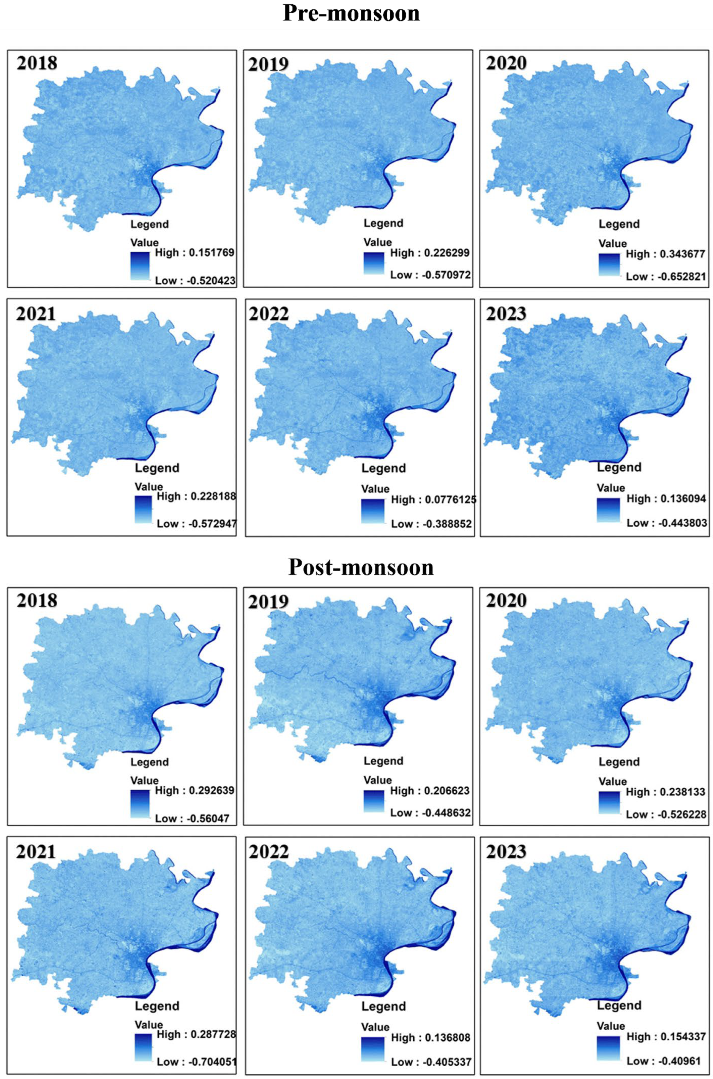
The NDWI consistently demonstrated an inverse correlation with LST across all years in pre- and post-monsoon seasons, as shown in Table 1, suggesting that areas with higher water content, indicated by higher NDWI values, have lower surface temperatures. These findings underscore the critical role of water bodies in mitigating surface heating and regulating urban microclimates.

3.1.2. Vegetation’s Complex Relationship with LST: Insights from NDVI

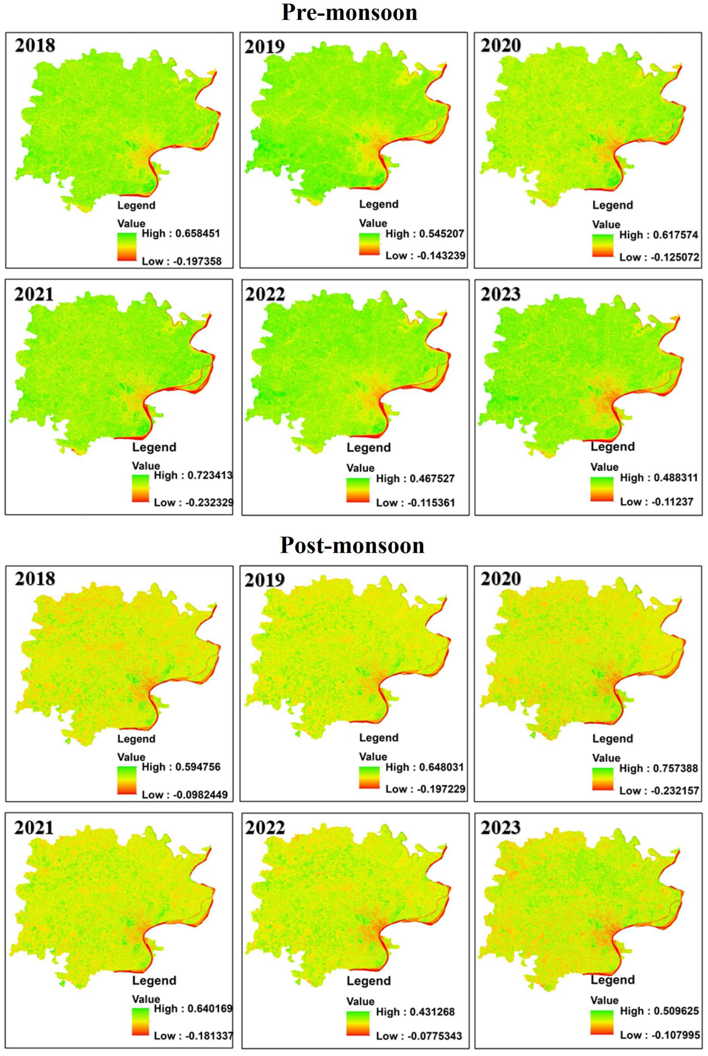
The Normalised Difference Vegetation Index (NDVI) shows a mixed correlation with LST, reflecting the complex interactions between vegetation and surface temperature. In the pre-monsoon seasons, the correlation fluctuates between −0.17 (2018) and 0.14 (2019). The post-monsoon values vary from −0.18 (2018) to 0.14 (2019). This variability is likely influenced by changes in vegetation health, density, and land cover over time. The years 2018 and 2021 show a negative correlation, implying that reduced vegetation is associated with higher temperatures. Whereas in 2019 and 2020, the positive correlation suggests higher temperatures in areas with increased vegetation. A positive correlation was observed between vegetation growth and the monsoon, but no cooling effect on surface temperature was noted because vegetation cover absorbs and reflects solar radiation.

3.1.3. Urbanisation and LST: Strong Correlation with NDBI

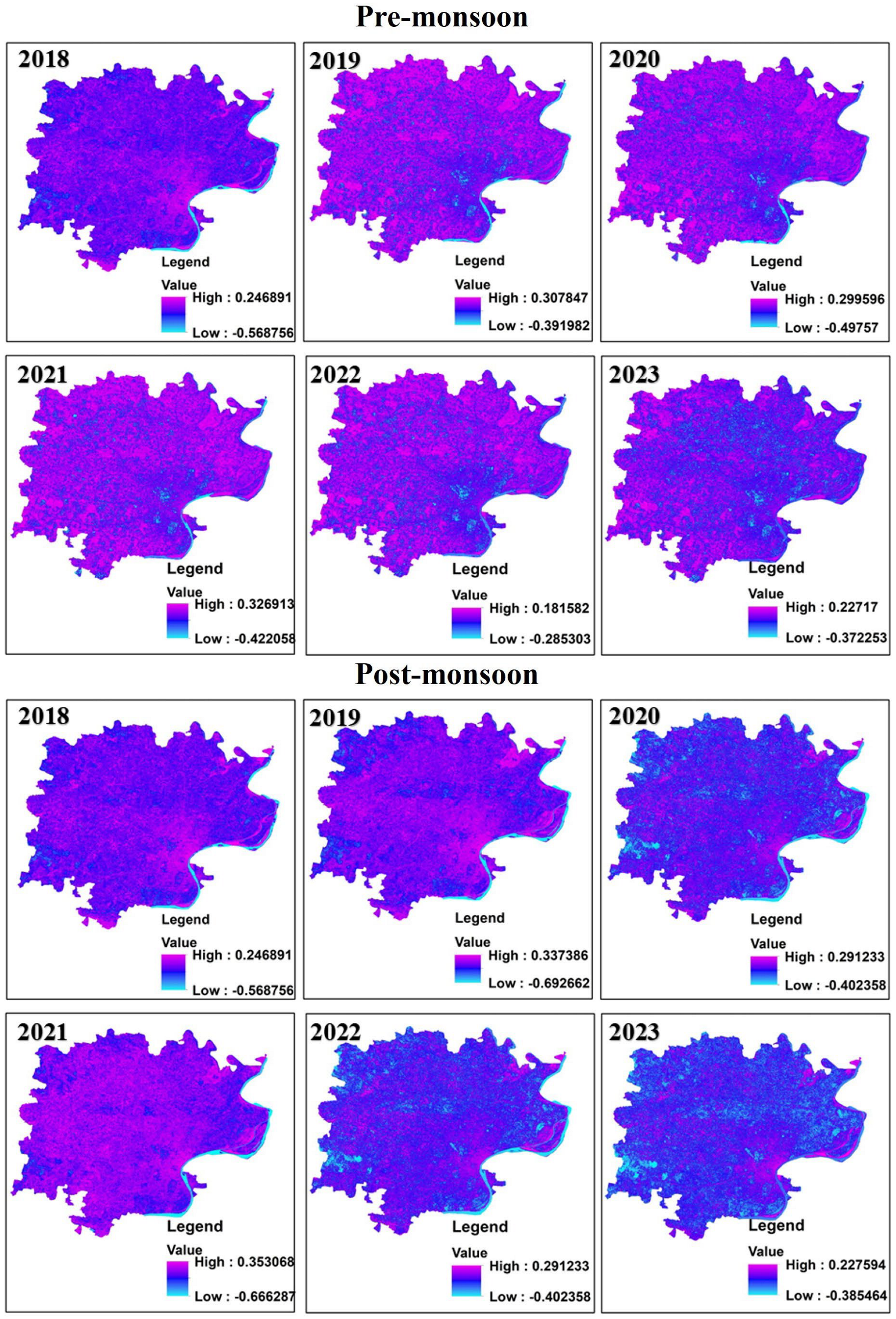
The Normalised Difference Built-Up Index (NDBI) exhibits a strong and consistent positive correlation with land surface temperature (LST) both in pre-monsoon and post-monsoon periods. The pre-monsoon correlation was 0.69 in 2018 and increased to 0.73 in 2023, while post-monsoon correlations varied from 0.48 in 2020 to 0.72 in 2019. This consistent correlation suggests that built-up areas, characterised by impervious surfaces such as concrete and asphalt, generally have higher surface temperatures, contributing to the urban heat island (UHI) effect. This relationship indicates the influence of urbanisation on surface warming and highlights the need for urban cooling strategies, such as increasing green spaces.

3.1.4. Role of Bare Soil in Elevating LST: Analysis of BSI

The correlation between the BSI and LST (Table 1) reveals a consistently strong positive relationship across both pre- and post-monsoon seasons, suggesting that areas with more bare soil experience higher surface temperatures compared to those with covered soil.
In the pre-monsoon period, BSI shows strong positive correlations with LST, ranging from 0.59 (2020) to 0.78 (2022). For the post-monsoon period, high correlation values of 0.79 and 0.53 were observed in 2019 and 2020, respectively. This positive correlation indicates that bare soil, which has lower moisture retention and higher heat absorption compared to that of vegetated areas, significantly contributes to surface heating.
The high BSI-LST correlation during the pre-monsoon season, when dry soil is present, suggests that land cover with exposed soil is more prone to heat stress. These findings are critical for urban planners, as areas with bare soil could increase urban heat island effects and contribute to localised warming. Urban planners can address the issue through land cover management—such as increasing vegetation or implementing soil moisture retention strategies to mitigate rising temperatures in urban areas like Varanasi.
The findings from Table 1 provide a detailed understanding of how different land cover types influence LST, which can inform planners in the development of effective strategies for managing urban areas and water resources.
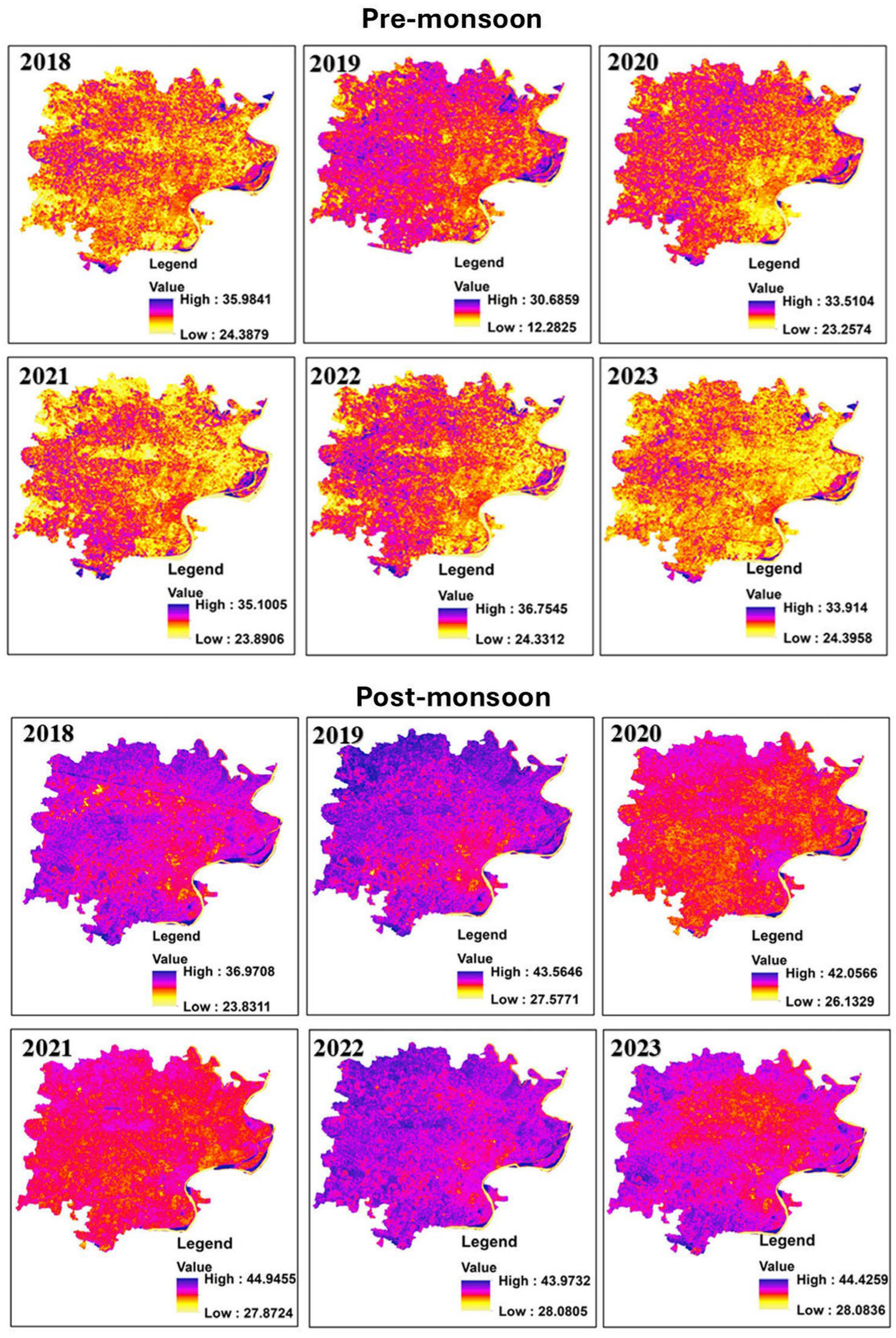
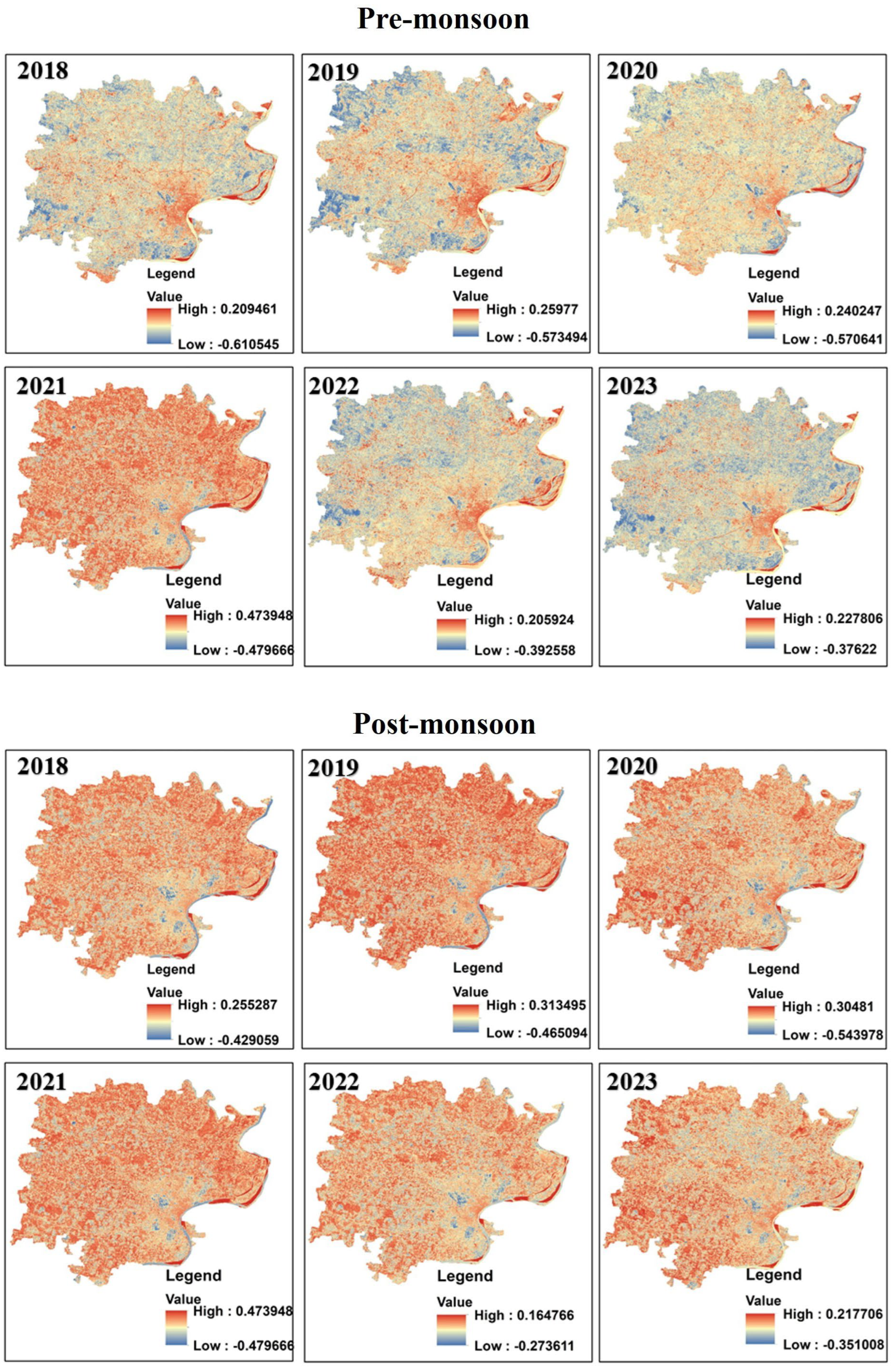
Figure 3, Figure 4, Figure 5, Figure 6 and Figure 7 represent the spatial variation in LST, NDVI, NDWI, NDBI, and BSI, respectively.

3.2. Performance of ML Algorithms for LST Prediction

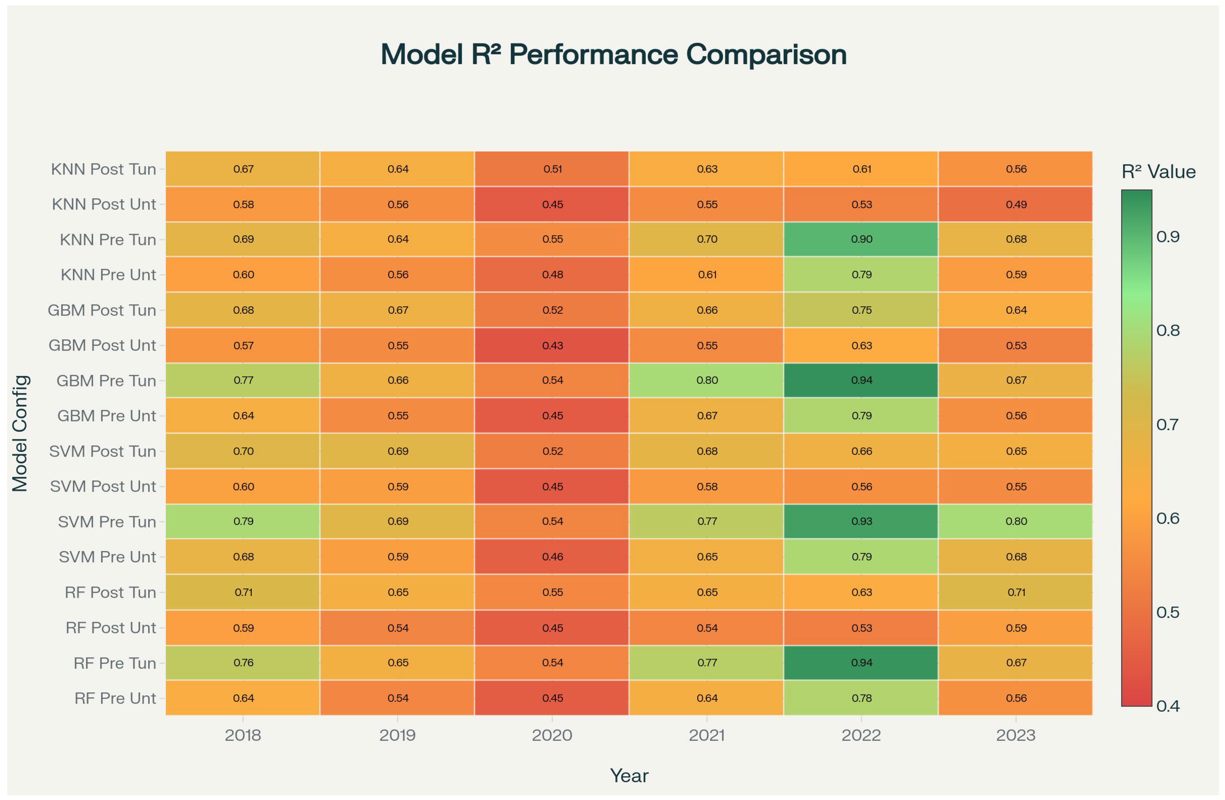
The R2 heatmap (Figure 8) reveals distinct seasonal performance patterns across all machine learning algorithms. For untuned models, pre-monsoon seasons consistently outperformed post-monsoon conditions. Random Forest achieved an average untuned R2 of 0.603 during the pre-monsoon season and 0.54 during the post-monsoon season. Support Vector Machine demonstrated similar trends, with pre-monsoon R2 averaging 0.642 and post-monsoon R2 averaging 0.556. Gradient Boosting Machine recorded pre-monsoon R2 of 0.608 and post-monsoon R2 of 0.544, while k-Nearest Neighbours showed pre-monsoon R2 of 0.602 and post-monsoon R2 of 0.527.
The year 2020 represented the most challenging prediction period across all algorithms, with R2 values dropping to their lowest points, ranging from 0.432 to 0.481, clearly visible as the darkest red band in the heatmap.
Hyperparameter tuning resulted in substantial performance improvements across all algorithms. The optimal hyperparameters are presented in Table 2. After optimisation, Random Forest achieved an average R2 of 0.724 during the pre-monsoon season and 0.649 during the post-monsoon season, representing improvements of 20.1% and 20.2%, respectively. Support Vector Machine demonstrated consistent improvement, with pre-monsoon R2 increasing to 0.753 and post-monsoon R2 to 0.651, marking increases of 17.3% and 17.1%, respectively.
Gradient Boosting Machine emerged as the top performer with a pre-monsoon R2 of 0.73 and a post-monsoon R2 of 0.653, showing improvements of 20.1% and 20.0% after hyperparameter tuning. K-Nearest Neighbours, while showing the most modest gains, still achieved meaningful improvements, with pre-monsoon R2 of 0.693 and post-monsoon R2 of 0.606, representing increases of 15.1% and 15.0% after hyperparameter tuning.
Random Forest (RF) reduced its Mean Absolute Error (MAE) from approximately 1.68 to 2.78 °C before tuning to 0.54 to 0.89 °C after tuning. The Mean Absolute Percentage Error (MAPE) dropped from about 0.56–0.74 to 0.45–0.54.
MAE for Support Vector Machine (SVM) decreased from 0.57–0.97 °C to 0.45–0.78 °C and MAPE reduced from 1.7–3.6 to 1.3–2.2. Gradient Boosting Machine (GBM) also improved, lowering MAE from around 0.59–1.04 °C to 0.47–0.75 °C, and MAPE from 1.8–3.8 to 1.4–1.9. k-Nearest Neighbours (KNN) showed the least improvement of all models; MAE decreased from 0.61–1.00 °C to 0.52–0.73 °C and MAPE decreased from 1.8–3.7 to 1.5–2.4. Errors were lower in pre-monsoon seasons than in post-monsoon seasons. The lower performance in 2020 is primarily due to cloud contamination in the paired scenes, which weakened index–LST consistency.
The error reduction following hyperparameter tuning was substantial and consistent across all models, as demonstrated in the boxplots (Figure 9). The tuned models (orange boxes) show markedly reduced median errors, compressed interquartile ranges, and fewer outliers compared to their untuned counterparts (blue boxes).
The analysis reveals that ensemble methods, notably Gradient Boosting Machine and Random Forest, can be optimal choices for LST prediction in an urban environment. As demonstrated for Varanasi, the selected area, these algorithms consistently delivered high accuracy (average R2 > 0.70). The substantial improvements achieved through hyperparameter optimisation enabled robust seasonal performance.
Support Vector Machine serves as a reliable alternative, offering consistent performance characteristics across various conditions. Meanwhile k-Nearest Neighbours, although improved through tuning, remains the least effective option for this specific application, achieving average R2 values around 0.65. However, it still provides acceptable predictive capability for particular scenarios.

4. Discussion

The results of this study highlight the effectiveness of machine learning algorithms in predicting LST in the context of Varanasi, India, across pre-monsoon and post-monsoon seasons. Among the algorithms tested, RF and SVM consistently demonstrated robust performance in predicting LST, underscoring their reliability for environment management applications. The higher R2 values and lower MAPE suggest that these algorithms can accurately model the complex relationships between LST and spectral indices such as NDVI, NDBI, NDWI, and BSI.
The strong positive correlation between NDBI and LST across seasons suggests that urbanisation, as indicated by increased built-up areas, is a significant contributor to surface temperature rise. This finding is critical for urban planners as it emphasises the importance of integrating different UHI mitigation strategies (such as increasing vegetation and reducing impervious surfaces) in city planning to manage rising temperatures. On the other hand, NDVI showed mixed correlations with LST, reflecting the complex interactions between vegetation and surface temperature. This study suggests that vegetation generally has a cooling effect, but its influence on LST can vary depending on the type, health, and density of the vegetation.
As represented by the NDWI, water bodies consistently demonstrated a negative correlation with LST, confirming their role in cooling urban environments. This finding highlights the importance of preserving and expanding water bodies in urban planning to mitigate UHI effects on desired surface temperatures.
Hyperparameter tuning proved essential in minimising both absolute and relative errors in LST prediction models. Ensemble models, such as RF and GBM, benefited the most, with error reductions of up to 30%, indicating their sensitivity to parameters like tree number, depth, and learning rates. SVM demonstrated moderate but meaningful improvements, especially in relative error metrics, while KNN showed limited adaptability but improved its accuracy post-tuning. These improvements translate to more reliable and precise LST estimations, critical for effective urban climate monitoring and environmental management. The tuned models’ enhanced stability and lower error variability support their practical use, highlighting hyperparameter optimisation as a necessary step for deploying ML models in Earth surface temperature applications.

4.1. Importance of LST Prediction in Environmental Management

Accurate LST prediction is pivotal in environmental management, particularly in mitigating UHI and addressing climate change. The findings underscore the critical role those spectral indices, especially the NDBI and NDVI, play in influencing LST dynamics. The strong positive correlation between the NDBI and LST emphasises the contribution of urbanisation to elevated surface temperatures, highlighting the urgent need for sustainable urban planning strategies to reduce heat stress. Similarly, the mixed correlation trends of the NDVI suggest that vegetation health and coverage have a significant influence on surface cooling, emphasising the importance of increasing green spaces in urban environments. The strong positive correlation between the NDBI and LST observed in this study aligns with previous findings by [25,32], which also demonstrated that increased built-up density and impervious surface fraction lead to elevated land surface temperatures.
LST prediction also helps in tracking surface energy balance and hydrological cycles. The negative correlation between NDWI and LST indicates that areas with lower water content exhibit higher surface temperatures, providing crucial insights for managing water resources and developing surface cooling strategies in arid and semi-arid regions.

4.2. Societal Implications of LST Management

Managing LST effectively can have profound societal impacts, especially in urban areas prone to heat stress and associated health risks. Comfortable temperatures are crucial for reducing heat-related mortality and improving public health. By predicting and mapping thermal hotspots, policymakers and urban planners can design energy-efficient urban areas. Targeted interventions such as planting trees, expanding green spaces and developing reflective surfaces can be implemented to manage surface temperatures. Singapore’s urban vegetation corridors demonstrate successful applications of LST-based urban heat mitigation.
Moreover, the findings are particularly relevant for Varanasi, a rapidly urbanising city where population growth and land use changes exacerbate the UHI effect. Mitigation strategies based on LST predictions can improve quality of life by lowering indoor cooling costs, reducing heat exposure, and supporting resilient urban development.

4.3. Limitations and Future Research Directions

NDVI–LST correlations can vary with canopy structure, moisture/irrigation, phenology, and mixed pixels; therefore, NDVI alone is not sufficient. Consequently, other multi-index predictors (NDWI/NDBI/BSI) should be combined to provide a reliable analysis. However, residual bias may arise from atmospheric variability, emissivity assumptions and downscaling despite near-coincident pairing and sub-pixel co-registration. Therefore, site-specific recalibration is advised before transfer. High-resolution LST maps (10 m) support the identification of hotspot areas (such as roofs, plants, parks, etc.) to prioritise mitigation strategies in urban planning.
This study demonstrated the effectiveness of ML models in predicting LST; however, it faced certain limitations. The resolution and availability of satellite data, particularly the lack of high-resolution thermal imagery, constrained the analysis. Future research should incorporate additional non-imaging parameters, such as soil moisture, air circulation, and solar radiation, to further improve model accuracy. Expanding the scope of study to peri-urban and rural areas would also provide more comprehensive insights into the regional heat island effects and their mitigation.

5. Conclusions

The prediction of LST using remote sensing spectral indices and machine learning techniques holds significant environmental and societal value. The approach presented in this study uses data-driven insights from models and simulations. Machine learning, particularly gradient boosting machines (GBMs), plays a critical role in accurately forecasting LST through indices such as the NDVI, NDWI, and NDBI.
Precise LST predictions are crucial for understanding and mitigating the UHI effect, which exacerbates the impacts of climate change. Environmentally, LST influences ecosystem management by affecting surface energy balance, soil moisture, and evapotranspiration processes. The strong association between LST and urbanisation, as captured by indices like the NDBI, highlights the need for sustainable urban planning in fast-growing cities. Targeting heat islands and thermally stressed zones enables urban planners to prioritise green infrastructure and cooling strategies, reducing surface temperatures and enhancing resilience against heat waves. From a societal perspective, improved management of LST through informed environmental policies can significantly enhance public health by reducing heat stress and heat-related mortality during extreme weather events.
It is shown that hyperparameter tuning substantially elevates the performance of machine learning models, particularly GBM and Random Forest, by optimising their ability to capture complex spectral–temperature relationships and reducing prediction errors, such as MAE and MAPE. These tuning enhancements ensure robust and reliable LST forecasting, supporting climate adaptation strategies that promote sustainable urban environments.
This methodology presents an urban planning framework that uses advanced land surface dynamics analysis and machine learning to help create comfortable and resilient cities by balancing environmental, climate, and human needs.

Author Contributions

Conceptualisation, A.M. and A.O.; methodology, A.M.; software, A.M.; formal analysis. A.M.; investigation, A.M. and N.S.; data curation, A.M.; writing—original draft preparation, A.M.; writing—review and editing, A.O. and R.K.C.; visualisation, A.M.; supervision, P.K.S. and A.O.; project administration, R.K.C. and A.O.; funding acquisition, R.K.C. All authors have read and agreed to the published version of the manuscript.

Funding

The research stay of Anurag Mishra at UiT was funded by BRIDGE (Project No.: 322325) and the publication charges are paid by UiT, Norway.

Institutional Review Board Statement

Not applicable.

Informed Consent Statement

Not applicable.

Data Availability Statement

Satellite datasets were accessed through the GEE platform. https://earthengine.google.com (accessed on 30 March 2024).

Acknowledgments

The authors are highly grateful to the Department of Civil Engineering, Indian Institute of Technology (BHU), for providing facilities for this study. The authors gratefully acknowledge Harsh Vardhan Badaya (Roll No. 20065139) for his assistance in preliminary data collection. The authors also thank the anonymous reviewers for giving valuable suggestions.

Conflicts of Interest

The authors declare no conflicts of interest.

Abbreviations

The following abbreviations are used in this manuscript:
LSTLand Surface Temperature
NDVINormalised Difference Vegetation Index
NDBINormalized Difference Built-up Index
NDWINormalized Difference Water Index
BSIBare Soil Index
RFRandom Forest
SVMSupport Vector Machine
KNNK-Nearest Neighbours
GBMGradient Boosting Machine

References

  1. Li, Z.-L.; Tang, B.-H.; Wu, H.; Ren, H.; Yan, G.; Wan, Z.; Trigo, I.F.; Sobrino, J.A. Satellite-derived land surface temperature: Current status and perspectives. Remote Sens. Environ. 2013, 131, 14–37. [Google Scholar] [CrossRef]
  2. Crago, R.D.; Qualls, R.J. Use of land surface temperature to estimate surface energy fluxes: Contributions of Wilfried Brutsaert and collaborators. Water Resour. Res. 2014, 50, 3396–3408. [Google Scholar] [CrossRef]
  3. Faisal, A.A.; Al Kafy, A.; Al Rakib, A.; Akter, K.S.; Jahir, D.M.A.; Sikdar, M.S.; Ashrafi, T.J.; Mallik, S.; Rahman, M.M. Assessing and predicting land use/land cover, land surface temperature and urban thermal field variance index using Landsat imagery for Dhaka Metropolitan area. Environ. Chall. 2021, 4, 100192. [Google Scholar] [CrossRef]
  4. Frahmand, A.S.; Akyuz, D.E.; Sanli, F.B.; Balcik, F.B. Can remote sensing and sebal fill the gap on evapotranspiration? A case study: Kunduz catchment, Afghanistan. J. Environ. Prot. Ecol. 2020, 21, 423–432. [Google Scholar]
  5. de Almeida, C.R.; Teodoro, A.C.; Gonçalves, A. Study of the urban heat island (Uhi) using remote sensing data/techniques: A systematic review. Environments 2021, 8, 105. [Google Scholar] [CrossRef]
  6. Mathew, A.; Sreekumar, S.; Khandelwal, S.; Kumar, R. Prediction of land surface temperatures for surface urban heat island assessment over Chandigarh city using support vector regression model. Sol. Energy 2019, 186, 404–415. [Google Scholar] [CrossRef]
  7. Megna, Y.S.; Pallarés, S.; Sánchez-Fernández, D. Conservation of aquatic insects in Neotropical regions: A gap analysis using potential distributions of diving beetles in Cuba. Aquat. Conserv. Mar. Freshw. Ecosyst. 2021, 31, 2714–2725. [Google Scholar] [CrossRef]
  8. Sánchez, J.M.; Galve, J.M.; González-Piqueras, J.; López-Urrea, R.; Niclòs, R.; Calera, A. Monitoring 10-m LST from the combination MODIS/Sentinel-2, validation in a high contrast semi-arid agroecosystem. Remote Sens. 2020, 12, 1453. [Google Scholar] [CrossRef]
  9. Reiners, P.; Sobrino, J.; Kuenzer, C. Satellite-Derived Land Surface Temperature Dynamics in the Context of Global Change—A Review. Remote Sens. 2023, 15, 1857. [Google Scholar] [CrossRef]
  10. Li, Z.L.; Wu, H.; Duan, S.B.; Zhao, W.; Ren, H.; Liu, X.; Leng, P.; Tang, R.; Ye, X.; Zhu, J.; et al. Satellite Remote Sensing of Global Land Surface Temperature: Definition, Methods, Products, and Applications. Rev. Geophys. 2023, 61, e2022RG000777. [Google Scholar] [CrossRef]
  11. Taloor, A.K.; Manhas, D.S.; Chandra Kothyari, G. Retrieval of land surface temperature, normalized difference moisture index, normalized difference water index of the Ravi basin using Landsat data. Appl. Comput. Geosci. 2021, 9, 100051. [Google Scholar] [CrossRef]
  12. Claverie, M.; Ju, J.; Masek, J.G.; Dungan, J.L.; Vermote, E.F.; Roger, J.-C.; Skakun, S.V.; Justice, C. The Harmonized Landsat and Sentinel-2 surface reflectance data set. Remote Sens. Environ. 2018, 219, 145–161. [Google Scholar] [CrossRef]
  13. Kim, M.; Cho, K.; Kim, H.; Kim, Y. Spatiotemporal Fusion of High Resolution Land Surface Temperature Using Thermal Sharpened Images from Regression-Based Urban Indices. ISPRS Ann. Photogramm. Remote Sens. Spat. Inf. Sci. 2020, V-3-2020, 247–254. [Google Scholar] [CrossRef]
  14. Zhang, L.; Yao, Y.; Bei, X.; Li, Y.; Shang, K.; Yang, J.; Guo, X.; Yu, R.; Xie, Z. ERTFM: An Effective Model to Fuse Chinese GF-1 and MODIS Reflectance Data for Terrestrial Latent Heat Flux Estimation. Remote Sens. 2021, 13, 3703. [Google Scholar] [CrossRef]
  15. Pu, R. Assessing scaling effect in downscaling land surface temperature in a heterogenous urban environment. Int. J. Appl. Earth Obs. Geoinf. 2021, 96, 102256. [Google Scholar] [CrossRef]
  16. Zegaar, A.; Telli, A.; Ounoki, S.; Shahabi, H.; Rueda, F. Data-driven approach for land surface temperature retrieval with machine learning and sentinel-2 data. Remote Sens. Appl. Soc. Environ. 2024, 36, 101357. [Google Scholar] [CrossRef]
  17. Shirgholami, M.R.; Masoodian, S.A.; Montazeri, M. Investigation of environmental changes in arid and semi-arid regions based on MODIS LST data (case study: Yazd province, central Iran). Arab. J. Geosci. 2023, 16, 514. [Google Scholar] [CrossRef]
  18. Shukla, K.K.; Attada, R.; Kumar, A.; Kunchala, R.K.; Sivareddy, S. Comprehensive analysis of thermal stress over northwest India: Climatology, trends and extremes. Urban Clim. 2022, 44, 101188. [Google Scholar] [CrossRef]
  19. Kumar, A.; Agarwal, V.; Pal, L.; Chandniha, S.K.; Mishra, V. Effect of Land Surface Temperature on Urban Heat Island in Varanasi City, India. J 2021, 4, 420–429. [Google Scholar] [CrossRef]
  20. Onačillová, K.; Gallay, M.; Paluba, D.; Péliová, A.; Tokarčík, O.; Laubertová, D. Combining Landsat 8 and Sentinel-2 Data in Google Earth Engine to Derive Higher Resolution Land Surface Temperature Maps in Urban Environment. Remote Sens. 2022, 14, 4076. [Google Scholar] [CrossRef]
  21. Main-Knorn, M.; Pflug, B.; Louis, J.; Debaecker, V.; Müller-Wilm, U.; Gascon, F. Sen2Cor for Sentinel-2. In Proceedings of the Image and Signal Processing for Remote Sensing XXIII, Warsaw, Poland, 11–14 September 2017; p. 3. [Google Scholar] [CrossRef]
  22. Valor, E.; Caselles, V. Mapping land surface emissivity from NDVI: Application to European, African, and South American areas. Remote Sens. Environ. 1996, 57, 167–184. [Google Scholar] [CrossRef]
  23. Rad, A.M.; Kreitler, J.; Sadegh, M. Augmented Normalized Difference Water Index for improved surface water monitoring. Environ. Model. Softw. 2021, 140, 105030. [Google Scholar] [CrossRef]
  24. Yao, Y.; Lu, L.; Guo, J.; Zhang, S.; Cheng, J.; Tariq, A.; Liang, D.; Hu, Y.; Li, Q. Spatially Explicit Assessments of Heat-Related Health Risks: A Literature Review. Remote Sens. 2024, 16, 4500. [Google Scholar] [CrossRef]
  25. Weng, Q.; Lu, D.; Schubring, J. Estimation of land surface temperature–vegetation abundance relationship for urban heat island studies. Remote Sens. Environ. 2004, 89, 467–483. [Google Scholar] [CrossRef]
  26. Mzid, N.; Pignatti, S.; Huang, W.; Casa, R. An Analysis of Bare Soil Occurrence in Arable Croplands for Remote Sensing Topsoil Applications. Remote Sens. 2021, 13, 474. [Google Scholar] [CrossRef]
  27. Breiman, L. Random Forests. Mach. Learn. 2001, 45, 5–32. [Google Scholar] [CrossRef]
  28. Raj, D.K.; Gopikrishnan, T. Machine learning models for predicting vegetation conditions in Mahanadi River basin. Environ. Monit. Assess. 2023, 195, 1401. [Google Scholar] [CrossRef]
  29. Song, Y.; Liang, J.; Lu, J.; Zhao, X. An efficient instance selection algorithm for k nearest neighbor regression. Neurocomputing 2017, 251, 26–34. [Google Scholar] [CrossRef]
  30. Ferreira, A.J.; Figueiredo, M.A.T. Boosting Algorithms: A Review of Methods, Theory, and Applications BT—Ensemble Machine Learning: Methods and Applications; Zhang, C., Ma, Y., Eds.; Springer: New York, NY, USA, 2012; pp. 35–85. [Google Scholar]
  31. Wang, B.; Hipsey, M.R.; Oldham, C. ML-SWAN-v1: A hybrid machine learning framework for the concentration prediction and discovery of transport pathways of surface water nutrients. Geosci. Model Dev. 2020, 13, 4253–4270. [Google Scholar] [CrossRef]
  32. Guha, S.; Govil, H.; Taloor, A.K.; Gill, N.; Dey, A. Land surface temperature and spectral indices: A seasonal study of Raipur City. Geod. Geodyn. 2022, 13, 72–82. [Google Scholar] [CrossRef]
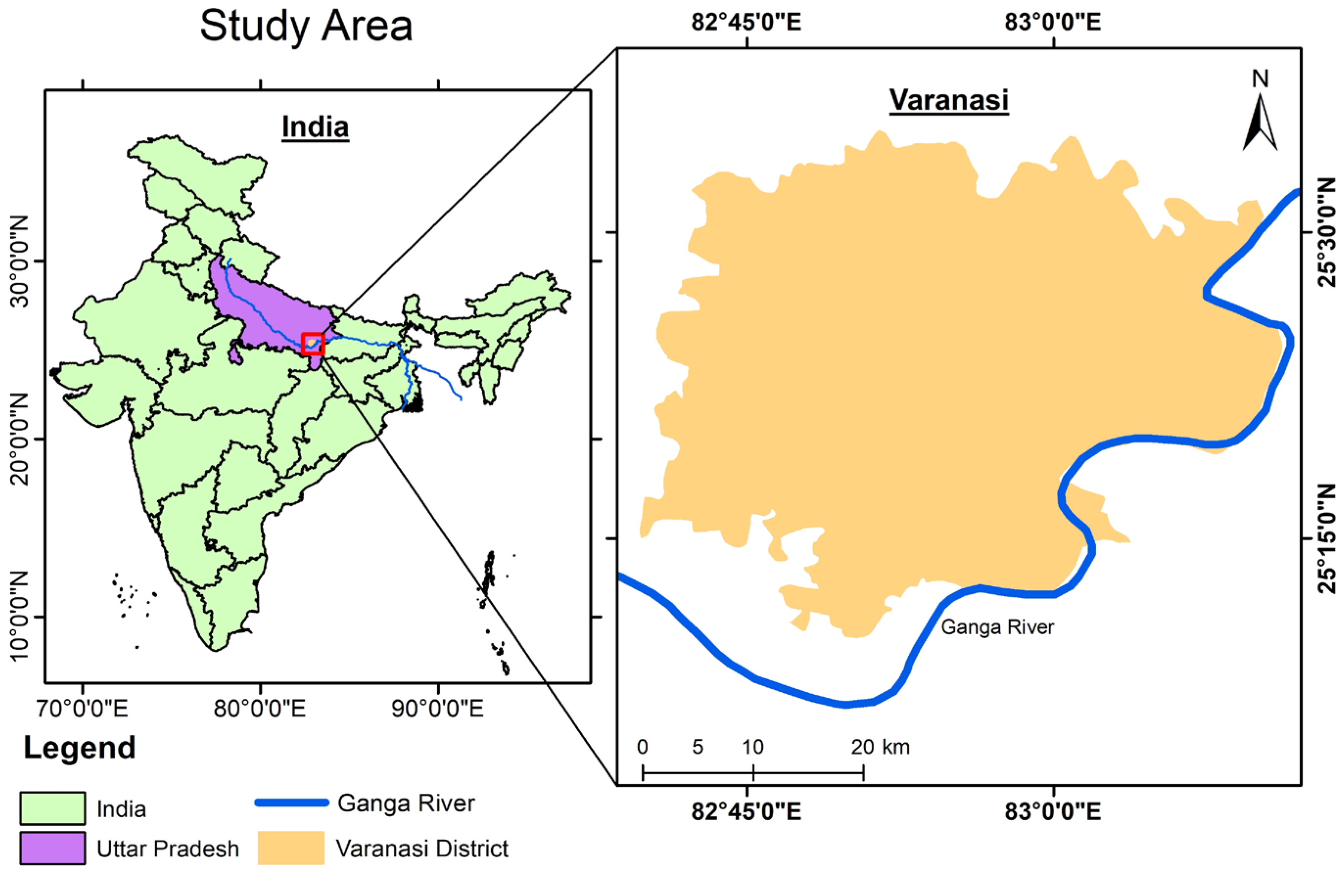
Figure 1. Study area map.
Atmosphere 16 01295 g001
Figure 2. Work Methodology.
Atmosphere 16 01295 g002
Figure 3. Seasonal Distribution of LST (2018–2023).
Atmosphere 16 01295 g003
Figure 4. Seasonal Distribution of NDWI (2018–2023).
Atmosphere 16 01295 g004
Figure 5. Seasonal Distribution of NDVI (2018–2023).
Atmosphere 16 01295 g005
Figure 6. Seasonal Distribution of NDBI (2018–2023).
Atmosphere 16 01295 g006
Figure 7. Seasonal Distribution of BSI (2018–2023).
Atmosphere 16 01295 g007
Figure 8. Heatmap of R2 values by year (2018–2023), model, and season.
Atmosphere 16 01295 g008
Figure 9. Boxplots comparing the distribution of MAPE (left) and MAE (right) for untuned and tuned models (RF, SVM, GBM, and KNN).
Atmosphere 16 01295 g009
Table 1. Correlation between the spectral indices and LST (coefficient based on linear relationship).
Pre-MonsoonPost-Monsoon
201820192020202120222023201820192020202120222023
NDWI−0.17−0.27−0.2−0.23−0.35−0.29−0.03−0.28−0.12−0.01−0.15−0.23
NDVI−0.170.140.03−0.06−0.04−0.13−0.180.14−0.05−0.140.03−0.09
NDBI0.690.720.530.550.710.730.690.720.480.670.650.68
BSI0.730.670.590.680.780.590.740.790.530.680.530.64
Table 2. Optimum hyperparameters for different ML algorithms.
ModelSeasonOptimum Hyperparameters
Random ForestPre-monsoonn_estimators = 300–500, max_depth = 8–10, min_samples_split = 2, min_samples_leaf = 1
Post-monsoonn_estimators = 300–500, max_depth = 8–10, min_samples_split = 2, min_samples_leaf = 1
Gradient Boosting MachinePre-monsoonn_estimators = 400–500, max_depth = 6–8, learning rate = 0.01–0.05, min_samples_split = 2, min_samples_leaf = 1
Post-monsoonn_estimators = 400–500, max_depth = 6–8, learning rate = 0.01–0.05, min_samples_split = 2, min_samples_leaf = 1
Support Vector MachinePre-monsoonKernel = ‘rbf’, C = 10–100, epsilon = 0.01–0.05, gamma = ‘scale’/’auto’
Post-monsoonKernel = ‘rbf’, C = 10–100, epsilon = 0.01–0.05, gamma = ‘scale’/’auto’
k-Nearest NeighboursPre-monsoonn_neighbors = 5–7, weights = ‘distance’, p = 2, algorithm = ‘auto’
Post-monsoonn_neighbors = 5–7, weights = ‘distance’, p = 2, algorithm = ‘auto’
Disclaimer/Publisher’s Note: The statements, opinions and data contained in all publications are solely those of the individual author(s) and contributor(s) and not of MDPI and/or the editor(s). MDPI and/or the editor(s) disclaim responsibility for any injury to people or property resulting from any ideas, methods, instructions or products referred to in the content.