Article

High-Resolution Traffic Flow Prediction and Vehicle Emission Inventory Estimation for Chinese Cities Using Geo-Spatial Data of Jinan City, China

1
Jinan Ecological and Environment Monitoring Center of Shandong Province, Jinan 250000, China
2
Beijing Smart Green Transport Research Centre, Beijing 100022, China
3
Energy Innovation: Policy and Technology, LLC, Energy Innovation 98 Battery Street, San Francisco, CA 94111, USA
4
Key Laboratory for Vehicle Emission Control and Simulation of Ministry of Ecology and Environment, Chinese Research Academy of Environmental Sciences, Beijing 100012, China
5
National Laboratory of Automotive Performance & Emission Test, School of Mechanical Engineering, Beijing Institute of Technology, Beijing 100081, China
*
Author to whom correspondence should be addressed.
Atmosphere 2025, 16(10), 1213; https://doi.org/10.3390/atmos16101213
Submission received: 15 August 2025 / Revised: 10 September 2025 / Accepted: 17 October 2025 / Published: 20 October 2025
(This article belongs to the Special Issue Recent Advances in Mobile Source Emissions (2nd Edition))

Abstract

Motor vehicle emissions are a major air quality concern in Chinese cities. However, traditional population-based emission inventory methods fail to capture the spatial and temporal variations in emissions for effective policy design. This study proposes a high-resolution approach for traffic flow prediction and vehicle emission inventory estimation, using Jinan City, China, as a case study. We leverage multi-source geospatial data and employ a two-fold random forest model to predict hourly traffic flow at a road-segment level. Speed-aligned emission factors were then combined with these data to calculate hourly and road-level vehicle emission estimates. Compared to traditional methods, our approach offers substantial improvements: (1) improved spatiotemporal resolution; (2) enhanced accuracy of traffic flow prediction; and (3) support for more effective vehicle emission control strategies. Results show that heavy-duty vehicles, particularly freight trucks operating on inter-regional corridors through Jinan, contribute 78% more to NOX emissions than local light-duty vehicles. These transient emissions are typically overlooked in static inventories but constitute a significant source of urban pollution. This study offers valuable insights for combining geospatial data and machine learning to improve the accuracy and resolution of vehicle emission inventories, supporting urban air quality policy and planning.

1. Introduction

Traffic emissions currently represent one of the main sources of air pollution in Chinese cities [1]. In some large and medium-sized cities, motor vehicles contribute to over 30% of nitrogen oxides (NOX) and over 20% of particulate matter (PM10 and PM2.5) [2,3]. In response, the Chinese government has consecutively introduced and strengthened multiple policy measures, including “Action Plan for Air Pollution Prevention and Control” and the “Three Year Action Plan for Blue Sky Defense” in 2013, and the “Air Pollution Prevention and Control Law” revised in 2018, which provided a solid legal foundation for the treatment of motor vehicle exhaust emissions [4,5]. Meanwhile, emissions of nitrogen oxides and particulate matter related to transportation have a direct impact on human health. Epidemiological studies have linked NOX exposure to increased risks of asthma, reduced lung function, and other respiratory diseases, while fine particulate matter (PM2.5) is associated with cardiovascular morbidity and premature mortality [6,7]. Populations living near major roads are especially vulnerable, and sensitive groups such as children and the elderly are disproportionately affected. These well-documented health impacts underscore the urgency of improving the accuracy and resolution of traffic emission inventories to support evidence-based air quality management and public health protection. Therefore, it is important to accurately and timely characterize vehicle operations and emission profiles for air pollution control and achieving these policy goals.
Current methods for estimating vehicle activity and emissions remain limited in scope and granularity. Traditional emission inventory approaches in China are primarily developed using an aggregated estimation method, calculated as the product of the number of registered vehicles, average annual vehicle kilometers traveled (VKT), and average emission factors within a given jurisdiction [8]. While the increasing availability of emission data categorized by regulatory standards has gradually enhanced estimation accuracy, this approach remains inadequate for capturing the dynamic variations across regions, time periods, and vehicle categories [9]. The reliance on static estimates makes it difficult to evaluate local policy effectiveness and to design data-driven control strategies. For example, non-local transit vehicles, especially heavy-duty trucks, are often excluded from traditional regional inventories despite their large impact. Recent high-resolution analyses using full-sample trajectory data revealed that in certain counties, emissions from non-local heavy-duty trucks can exceed those from local vehicles by ~15 times, contributing up to 31% of regional truck emissions [10]. Additionally, although Portable Emission Measurement Systems (PEMSs) could provide high-frequency and vehicle-specific real-world emission data, their limited spatial coverage and sample size constrain their applicability for city-scale emission management [11]. Consequently, traditional estimation methods fall short in supporting real-time pollution forecasting and responsive policymaking. There is an urgent need for more dynamic, fine-grained models to support operational management and timely regulatory intervention.
Recent advances in high-resolution traffic modeling can enhance the capture of spatial and temporal variability of traffic flow and associated emissions. These developments are driven by the integration of intelligent transportation systems (ITSs), online mapping platforms, and real-time monitoring, which provide valuable and detailed data [12,13,14,15]. For example, Li et al. [16] utilized three machine learning algorithms: Random Forest, Gradient Boosting Decision Tree (GBDT), and Extreme Gradient Boosting (XGBoost), integrating taxi GPS and multi-source urban data, to conduct high-resolution spatiotemporal analysis of urban road traffic emissions. Similarly, Yang et al. [17] constructed a machine learning-based model to forecast surface concentrations of NO2, O3, and PM2.5 in the Los Angeles metropolitan area. However, several limitations remain related to data reliability and modeling robustness. ITS-derived data are often fragmented, inconsistently formatted, and lack standardization across regions, leading to uncertainty in emission estimation [18]. Additionally, inconsistent data formats, incomplete data fusion algorithms, and lack of long-term data acquisition lead to inaccurate big data analysis results [19,20]. Moreover, existing methods struggle to capture the stochastic and non-linear nature of urban traffic flow, especially under dynamic conditions such as congestion, weather disruptions, and policy interventions [21]. Machine learning methods provide powerful tools for traffic and emission modeling because they can capture complex, non-linear interactions between congestion, temporal variation, and traffic flow that are difficult to represent with traditional regression models [22,23,24]. While machine learning has shown potential for capturing these complexities, existing methods often rely on static historical datasets and lack robust practical deployment [25].
This study aims to build a high-resolution, transient, and accurate traffic monitoring model system through stable data flow. Based on this framework, multiple data sources including dynamic congestion index were gathered to develop a bottom–up spatiotemporal emission inventory. Through data preprocessing and the application of a Random Forest algorithm, vehicle emissions are estimated across the Jinan city at the road-segment level. This study provides a scientific basis for fine-grained assessment of environmental impacts and gives strong data support for real-time traffic emission management.

2. Data and Methodology

2.1. Technical Approach

Figure 1 presents the technical framework in this study. We achieved breakthroughs in several core aspects of the technological roadmap: (1) selected a continuous and stable congestion index as the fundamental input for the model, ensuring the data’s consistency and enabling real-time observation and computation; (2) accurately allocated the congestion index to each road segment using a Geographic Information System (GIS) system; (3) developed machine learning algorithms to dynamically and in real time convert the congestion index into traffic flow; and (4) constructed machine learning algorithms to enable the dynamic calculation of emission factors for individual road segments.

2.2. Data Collection and Processing

We constructed a geospatial dataset integrating road characteristics, land use, congestion levels, and traffic flow observations across 13,519 road segments in Jinan, China. Road infrastructure attributes (e.g., width, lane count, and classification) were extracted from OpenStreetMap and NavInfo. The points of interest (POIs), such as hospitals, schools, marketplaces, banks, and tourist attractions, were derived from Amap (Gaode Maps). The road congestion index was obtained from Baidu Maps covering November 2020, March 2021, and July 2021, with hourly values ranging from 1 (free flow) to 18 (severe congestion). The Baidu congestion index is an objective indicator of traffic congestion, officially defined by Baidu Maps Smart Transportation. It is calculated from large-scale traffic big data, including vehicle trajectories and location records from Baidu Map users. Specifically, the congestion index is defined as the ratio of actual travel time to free-flow travel time, where a larger value indicates a higher level of congestion (https://jiaotong.baidu.com/congestion/city/highwayrealtime/ (accessed on 8 September 2025)). Detailed information on datasets is presented in Appendix A.1. We preprocessed these data structured into a simplified single-line road network in a GIS environment (details in Appendix A.2). The road network dataset for Jinan comprises 13,519 road segments, covering the entire urban area with a cumulative road length of approximately 9935.3 km. The Baidu congestion index was incorporated directly as an explanatory variable through a length-weight segment average approach (details in Appendix A.3) to align with the simplified road network segmentation. This approach ensured consistency across data sources while preserving the raw temporal variation in the congestion index. Traffic congestion can effectively reflect traffic flow [26]. Its strong relevance to traffic flow prediction is further demonstrated by its consistent ranking as one of the most important features in driving prediction accuracy.
Observed traffic flow data were sourced from over 800 surveillance cameras managed by the Jinan Municipal Transportation Bureau. A two-stage process was used to assign intersection-level camera data to directional road segments. We mapped intersection-level data to road segments by estimating traffic volumes using nearby intersections and turning movements. For segments with dual-direction cameras, we aggregated flows to ensure consistency. For segments without camera observations, traffic flows were estimated using the Random Forest prediction model trained on segments with observed data and explanatory variables such as congestion index, road classification, and location characteristics. In this way, traffic flows for unmonitored segments were inferred rather than interpolated, ensuring that the entire road network was covered. Finally, automated license plate recognition (ALPR) systems installed at intersections were used to distinguish between light-duty vehicles (LDVs) and heavy-duty vehicles (HDVs). The classification was derived from plate number patterns combined with aggregated vehicle registration records provided by the Jinan Municipal Transportation authorities. Only anonymized and aggregated outputs were used in this study, and no personally identifiable license plate data were accessed. Detailed processing method of traffic flow is presented in Appendix A.4.
Speed-dependent emission factors by vehicle types, fuel types, and emission standards were derived for light-duty vehicles (LDVs) and On-Board Diagnostics (OBD) systems for heavy-duty vehicles (HDVs) [27], details in Appendix A.5. These factors were weighted by local fleet composition to reflect real-world traffic and emissions behavior. Vehicle composition was provided by the Jinan Environmental Protection Bureau and the Jinan Municipal Transportation Bureau provided these fleet composition data.
Appendix A provides detailed descriptions of the preprocessing procedures for all datasets used in this study. Road attribute data from OpenStreetMap and NavInfo were integrated and standardized into a simplified single-line network. Baidu congestion indices, sampled in November 2020, March 2021, and July 2021, were matched to the simplified network using a length-weighted averaging method to minimize biases caused by segmentation differences. Traffic flow data from more than 800 surveillance cameras were cleaned to exclude periods affected by equipment malfunction or incomplete recognition, and intersection-level counts were systematically assigned to directional road segments as described in Appendix A.4. Automated license plate recognition (ALPR) outputs were combined with local vehicle registration records to classify light- and heavy-duty vehicles for model training, with data access and governance described in Appendix A.4 and Appendix A.5. Speed-dependent emission factors were constructed by aligning VECC laboratory measurements with PEMS/OBD on-road data and weighted by the local fleet composition obtained from official statistics (Appendix A.5). The integration of VECC laboratory measurements with PEMS and OBD on-road datasets followed the procedures described in recent methodological studies [27,28], ensuring that the resulting emission factors reflect both controlled laboratory conditions and real-world driving behavior. The speed–emission factor relationship was modeled as a non-linear function empirically derived from these combined datasets, rather than assuming a simple linear dependence (Figure A3). These preprocessing and validation steps ensured the consistency, reliability, and suitability of the multi-source datasets for developing the high-resolution vehicle emission inventory.

2.3. Traffic Flow Machine Learning and Model Construction

Random forest (RF) was selected as the primary machine learning model in this study. RF is an ensemble learning method that constructs multiple decision trees and aggregates their outputs to improve predictive performance. The algorithm is particularly effective at modeling non-linear relationships and interactions among variables, while being relatively robust to overfitting. For model inputs, the predictor set included congestion index, temporal variables (hour of day, day of week, holiday indicators), and road attributes. The target variable was hourly directional traffic flow, expressed in passenger car equivalents (PCEs). Model hyperparameters, including the number of trees, maximum tree depth, and minimum samples per leaf, were optimized through grid search combined with five-fold cross-validation.
RF was chosen over alternative approaches for several reasons. Compared with linear regression, RF better captures the non-linear relationships between congestion, temporal patterns, and traffic flow. Compared with gradient boosting algorithms, RF requires less parameter tuning and is more robust when data volume is moderate. Neural networks offer strong flexibility but typically demand larger training datasets and longer training times, which were not available in this study. Given these trade-offs, RF was considered the most suitable choice for integrating heterogeneous, multi-source datasets in this context. This methodological design ensures that the model can leverage both congestion index and temporal factors to predict traffic flow with high accuracy, while maintaining computational efficiency and robustness.
Random forest was employed to model two variables: (1) total traffic flow expressed in PCEs, and (2) the ratio of light-duty to heavy-duty vehicles. In the first stage, total PCE per road segment was modeled as a function of input features (Appendix A.4). In the second stage, we predicted the proportion of private-car PCE in total PCE, using the same set of predictors. The final vehicle-type-specific traffic flows were derived by multiplying the predicted total PCE by the predicted ratio for private cars and its complement for heavy-duty vehicles.
Here, we set road features, environmental features near the road, and instantaneous value (time and congestion index) as the independent variables ( X ), and the proportions of PCE and PCE flow in each of the road segment as the dependent variables ( Y ) (details in Table A6). We chose the Random Forest Regressor package from scikit learn in Python 3.13 to simulate and predict the model. And we spatially joined the traffic flow data, based on camera locations, with the intersecting road segments to construct the initial training dataset. Model performance was evaluated using K-fold cross-validation to ensure robustness. Most hyperparameters remained at default values, except n_estimators, which was set to 1000 to reduce underfitting and enhance the model’s capacity to capture complex traffic patterns in the relatively small and noisy dataset.

2.4. Segment-Based Emissions

Speed-dependent emission factors were utilized to estimate hourly and segment-specific vehicle emissions influenced by traffic conditions. The total NOX emissions for each road segment i during time interval t were estimated using Equation (1). Based on the predicted traffic volumes and the speed-adjusted emission factors derived from laboratory and field monitoring data, we computed the dynamic vehicular emissions and spatially allocated them to corresponding road segments across the urban road network.
E i , t = v ( V i , t v × E F v s i , t × L i )
where  E i , t  is the estimated NOX emission (g) for the road segment i during time t V i , t v  is the traffic volume (vehicles/h) of vehicle category v (e.g., LDV or HDV) on road segment i at time t E F v s i , t  is the emission factor (g/km) for vehicle category v as a function of average speed  s i , t   L i  is the length of road segment i (km).

3. Results

3.1. Performance of Machine Learning

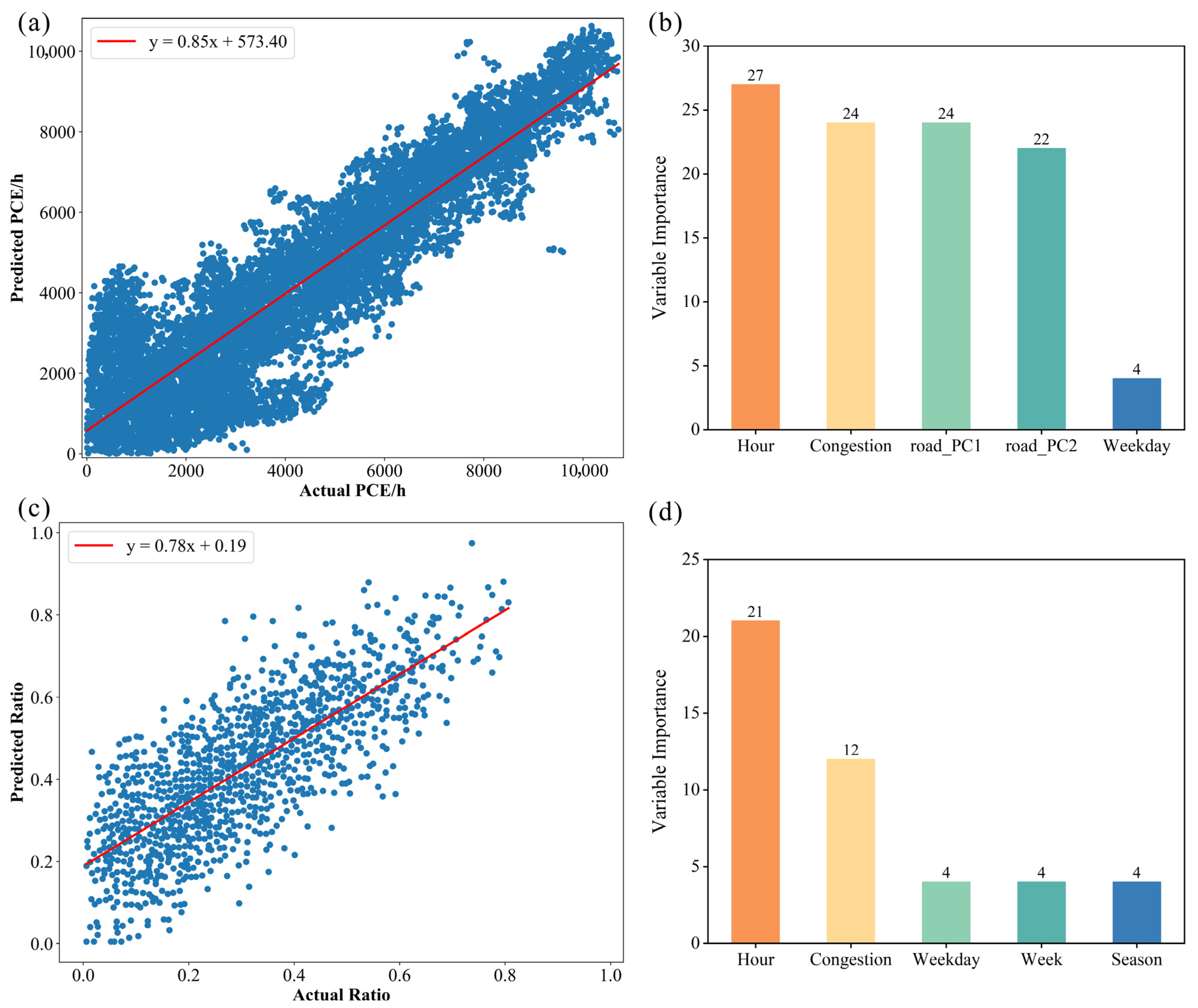
We applied a two-fold validation approach to verify the model, and the validation results are shown in Figure 2. Fold 1 focused on predicting total traffic flow in PCE units, while Fold 2 aimed to estimate the proportion of passenger cars within total traffic. In Fold 1, the model showed strong performance (R2 = 0.91), with predictions closely matching observed PCE values (Figure 2a). The major errors occurred in the low volume end (lower left end in Figure 2a), which reflect the fact that at the non-congested times—when vehicles operate in a traffic free flow mode—the congestion index is normally set as 1 to 2, thus it cannot reflect the vehicle speed and vehicle traffic flow. This situation normally happens in the evening, and the traffic flow is lower thus has less impacts on vehicle emissions and air quality. In this regard, we do not further iterate the model to avoid overfitting. In Fold 2, the model achieved moderate accuracy in predicting the passenger car share (R2 = 0.77, Figure 2c).
Figure 2b shows the top five impactful variables for Fold 1. The first and second principal components of road attributes represent the two features with the highest variance contribution obtained from the principal component analysis (PCA) of road data. The variable “hour” ranked first in importance, highlighting its critical role in capturing temporal dynamics. As a city known for its severe traffic congestion, Jinan exhibits strong time-dependent fluctuations in traffic flow, particularly during peak hours (e.g., 7:00–9:00 and 17:00–19:00). The PCE (Passenger Car Equivalent) essentially reflects traffic load per unit time, and the “hour” variable effectively captures the periodic variations in traffic demand. Furthermore, time-specific traffic control measures implemented in Jinan—such as peak-hour restrictions and odd-even license plate policies—contribute to pronounced differences in vehicle behavior across different times of day, thereby reinforcing the predictive power of this variable. The congestion index ranked second in variable importance, reflecting its strong influence on PCE. As a direct indicator of traffic efficiency and road utilization, congestion plays a critical role in shaping passenger car equivalent values. In Jinan—a city characterized by dense old urban areas, a complex road network, and high traffic volumes—congestion levels exhibit significant variability, especially along arterial roads and expressways. Importantly, congestion is not solely determined by vehicle volume; it is also influenced by signal timing, lane width, and incidental disruptions such as illegal parking or traffic accidents, which further enhance its explanatory power in the model.
Variables derived from road characteristics, such as those represented by principal components (e.g., road_PC1 and road_PC2), capture essential spatial features including land use intensity, road network density, and population distribution within defined buffer zones. The variable “weekday” received the lowest importance score but still contributes meaningful information to the model. Travel behavior in urban areas such as Jinan exhibits clear differences between weekdays and weekends. On weekdays (Monday to Friday), commuting patterns dominate, resulting in pronounced morning and evening peak traffic periods. In contrast, weekends are generally characterized by more discretionary and spatially dispersed travel, leading to different temporal and spatial traffic dynamics. Additionally, several traffic control policies in Jinan—such as license plate-based restrictions implemented on workdays—are explicitly tied to the day of the week. While the influence of “weekday” is less direct than other variables (e.g., hour or congestion), it nonetheless captures systematic variations in traffic demand and regulation that affect PCE.
For Fold 2, time-related variables played a crucial part in the vehicle type distribution (Figure 2d). The most important variable is also the hour, followed by congestion index and three other time related variables. It is worth noticing that congestion index played important roles in both models. Compared to the Fold 1 model, almost all the important viables besides the road characteristics are time-related variables. This reveals that HDVs running are organized and responses to the dispatching strategy and control policies from the owner and the government regardless the surrounding rode situation.
Based on the model’s tendency to overestimate the PCE ratio, particularly during periods when freight vehicles are more likely to be present, several implications can be drawn regarding traffic regulation and modeling. The dominant role of temporal variables, especially “hour”, suggests that Jinan’s current freight restriction policies, though effective in general, may benefit from more finely tuned temporal and spatial control measures. Real-time or dynamically adjusted freight restrictions, tailored to actual traffic conditions rather than fixed intervals, could improve model calibration and traffic adaptability. Moreover, the model’s bias highlights the need for more detailed data on freight movement, especially during transitional periods around restricted hours. Enhanced vehicle classification data would allow for better differentiation between permitted and restricted freight flows, thereby reducing prediction error and improving model accuracy.
In addition, the integration of traffic policy variables, such as restriction enforcement status or intensity, into the modeling framework, could further enhance predictive performance and enable robust scenario analysis. This would allow transportation planners to evaluate the potential impacts of policy changes before implementation. Finally, in light of the strong time-dependent patterns in traffic composition, policymakers are encouraged to promote off-peak logistics through targeted incentives or dynamic tolling strategies. The development of smart freight routing systems that align with regulatory constraints while minimizing network congestion would support more balanced and sustainable urban traffic management.

3.2. Spatiotemporal Characteristics of Traffic Flow Distribution

As illustrated in Figure 3, we analyzed the traffic flow across various road types in Jinan City and identified distinct spatial and temporal patterns for both light and heavy vehicles. We classified the road network into six categories: urban ring expressways, highways, national roads, provincial roads, county roads, and township roads, and recorded vehicle flows hourly over a 24 h period.
As shown in Figure 3d, the urban ring expressways exhibited concentrated traffic flows, particularly in the central and eastern regions. Light vehicle volumes peaked sharply at 914 vehicles/h around 8:00 a.m., corresponding to morning commuting hours. A secondary evening peak of 789 vehicles/h occurred around 6:00 p.m. In contrast, heavy vehicle volumes remained relatively stable throughout the day, fluctuating slightly around 85 vehicles/h, suggesting the effective implementation of vehicle restrictions during peak periods, in line with Jinan’s traffic control policies. On highways (Figure 3e), light vehicle traffic reached the highest peak among all road types, at 1306 vehicles/h around 8:00 a.m. Heavy vehicle volumes were also more pronounced than on the urban ring expressways, peaking at 151 vehicles/h, likely due to logistics and freight transport linked to intercity connections. The traffic distribution was geographically more dispersed, covering both urban and suburban fringe areas. Figure 3f showed that national roads functioned as major transport arteries with substantial light vehicle activity, peaking at 843 vehicles/h in the morning and remaining above 700 vehicles/h through midday. Heavy vehicle flows reached 74 vehicles/h, a moderate level compared to highways, reflecting more flexible freight movement allowed on national roads while still discouraging congestion in central urban areas. Provincial roads, shown in Figure 3g, exhibited traffic patterns similar to national roads but with slightly lower volumes. Light vehicles peaked at 840 vehicles/h, while heavy vehicles reached 80 vehicles/h. The spatial distribution was more uniform, serving both regional traffic and suburban commuting. These findings aligned with Jinan’s policy goal of decentralizing traffic away from core urban areas. As presented in Figure 3h, county roads displayed a light vehicle peak of 846 vehicles/h in the morning and 747 vehicles/h in the evening, with a pattern similar to but less intense than highways. Heavy vehicle traffic on county roads peaked at 73.33 vehicles/h, which was notably higher than on some higher-level roads. This trend possibly reflected rural freight movement and agricultural supply transport toward urban centers. Township roads, visualized in Figure 3i, carried the lowest traffic volumes, with light vehicle peaks at 851.34 vehicles/h and heavy vehicle peaks at 81.32 vehicles/h. Despite modest overall volumes, these roads were densely distributed in rural areas. The relatively strong morning peak suggested growing rural commuting and delivery activity, indicating an increasing role of township roads in supporting regional mobility. Across all road types, light vehicles exhibited a bimodal temporal pattern, with peaks during 7:00–9:00 a.m. and 5:00–7:00 p.m., consistent with commuter travel behavior. In contrast, heavy vehicle traffic remained relatively stable throughout the day, with moderate peaks that avoided rush hours. This trend demonstrated compliance with Jinan’s time-based vehicle restriction policies.
Spatially, heavy vehicle activity appeared more prominent on lower-grade roads, which may have reflected deliberate freight routing strategies intended to minimize congestion and pollution in the urban core. These findings affirmed the effectiveness of Jinan’s differentiated road-use strategy, where expressways and highways prioritized passenger vehicles during peak periods, while lower-grade roads accommodated a larger share of freight transport. Future transportation planning should continue to enhance traffic monitoring and optimize freight corridors to balance transportation efficiency with environmental and livability goals.
The traffic volume of both light-duty and heavy-duty vehicles in Jinan exhibits distinct variation patterns across different days of the week (Figure A4). Light vehicle traffic volume peaked on Monday (12,753.94 vehicles) and gradually declined over the workweek, reaching a minimum on Thursday (11,858.68 vehicles). This trend suggested a typical commuter-based pattern, in which weekday traffic was largely driven by work and school travel. Throughout the week, light vehicles consistently accounted for over 77% of total traffic volume, with only minor daily variation, highlighting their dominant role in Jinan’s daily mobility. This distribution aligned with the city’s vehicle restriction measures and green commuting policies, which promoted the use of public transit and staggered travel during peak periods, especially on key urban road segments. Heavy vehicle volumes remained relatively steady throughout the week but showed a gradual decrease from Monday (1438 vehicles) to Thursday (1294 vehicles). A moderate increase followed on Friday (1338 vehicles), with slightly lower volumes observed over the weekend. This midweek trough corresponded with freight traffic restrictions implemented on weekdays, which limited the daytime movement of heavy-duty trucks in order to reduce congestion and emissions within the urban core. Despite these restrictions, heavy vehicles consistently represented about 22–23% of the weekly traffic volume, underscoring their essential role in logistics and goods distribution—particularly on peripheral roadways and during nighttime hours. The consistent share of heavy vehicle traffic across the week, despite fluctuations in total vehicle volume, reflected the effectiveness of Jinan’s time-phased traffic control policies. These findings were critical for refining day-specific congestion mitigation strategies, optimizing road network operations, and enhancing the environmental outcomes of differentiated vehicle control policies.
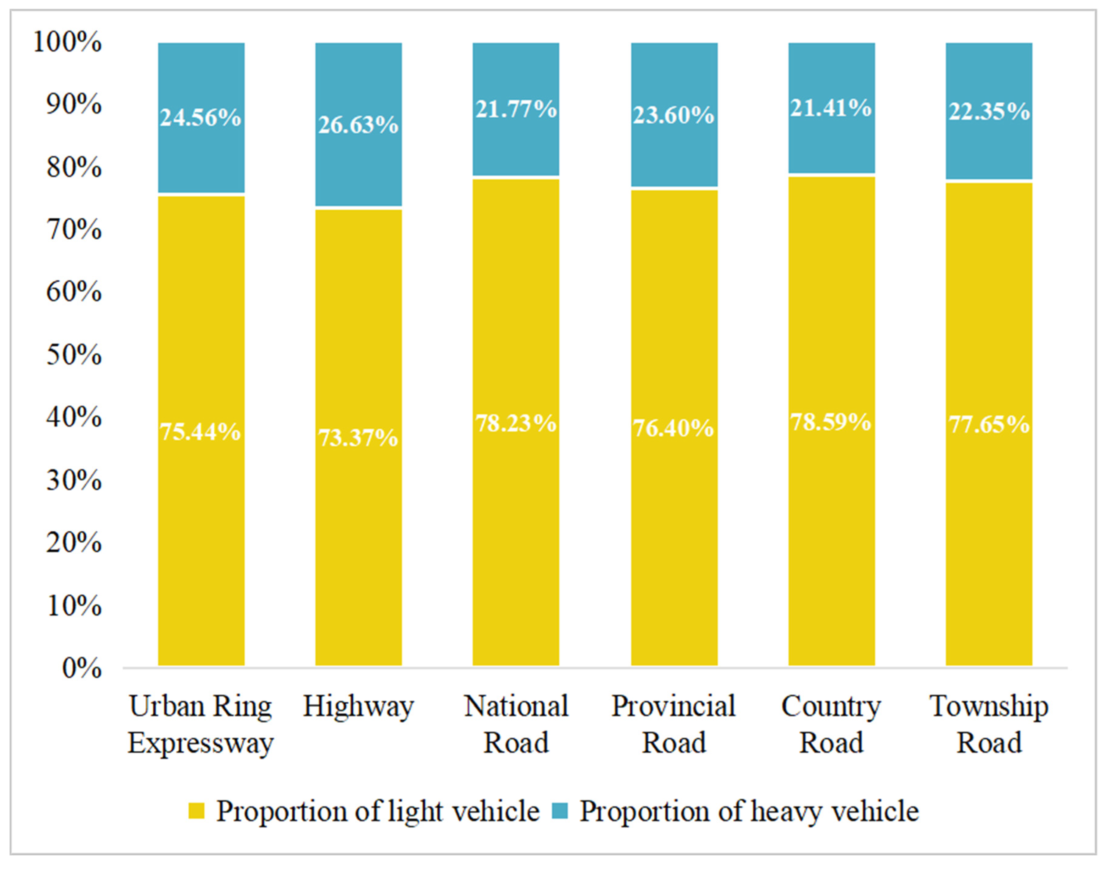
The traffic composition of light-duty and heavy-duty vehicles in Jinan shows slight differences across different road types (Figure A5). Light vehicles constituted the majority of traffic across all road types, ranging from 73.37% on highways to 78.59% on county roads. Heavy vehicles made up the remaining traffic share, with the highest proportions observed on highways (26.63%) and urban ring expressways (24.56%). These roads functioned as freight-preferred corridors, often situated outside of central traffic restriction zones. This reflected the city’s strategy to redirect truck traffic away from densely populated residential areas. The lower proportions of heavy vehicles on provincial (23.60%), township (22.35%), national (21.77%), and county (21.41%) roads indicated the effectiveness of time-based and zonal freight control policies—such as the “limited hours and areas for truck access” policy—that restricted large freight vehicles during peak hours and within urban districts.
The observed traffic flow distribution across road types supported the effectiveness of Jinan’s hierarchical road network and classification-based traffic policies. By concentrating heavy-duty freight traffic on high-capacity corridors (e.g., highways and expressways) and restricting it on lower-grade roads, the city achieved a balanced spatial allocation that facilitated both economic activity and urban livability. This strategy also aligned with national guidelines on urban freight zoning and vehicle-type planning, which aimed to ensure smoother traffic flow and reduced vehicle emissions in sensitive urban areas. Future transport planning could further reinforce the role of urban ring expressways as freight corridors while strengthening the enforcement of truck access restrictions within the internal urban road system.

3.3. Emission Inventory Results

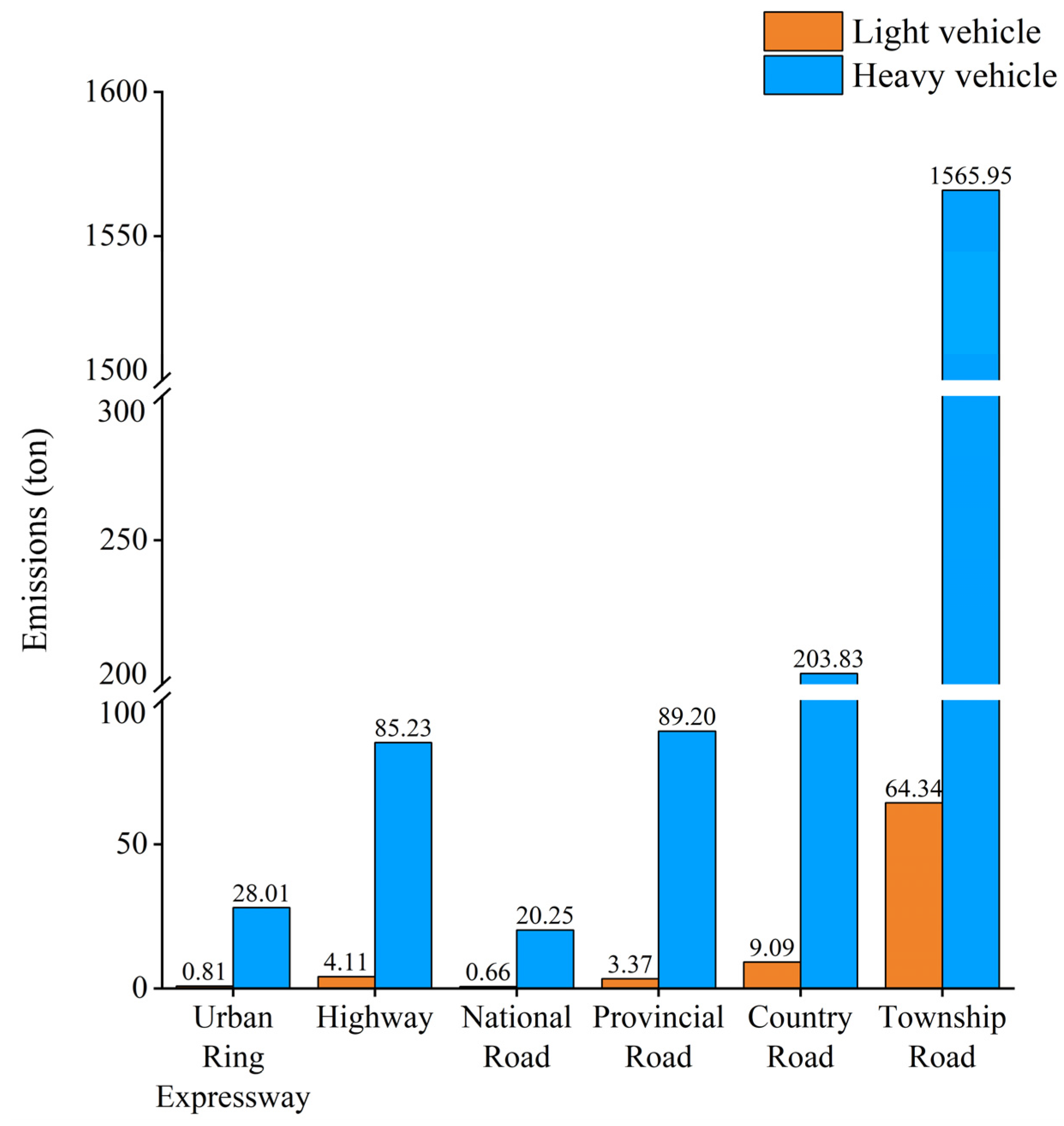
Figure 4 illustrated the spatial distribution of NOX emissions from light-duty and heavy-duty vehicles across the Jinan metropolitan area, along with the emission quantities classified by road type. NOX emissions from light-duty vehicles remained relatively low and more evenly distributed across the region. Hotspots primarily appeared in urban centers and along major transportation corridors. Emission levels ranged from 0 to 186.51 kg, with the highest concentrations occurring in areas with dense road networks and intense vehicle activity. In contrast, emissions from heavy-duty vehicles (Figure 4b) appeared more spatially clustered and showed significantly higher intensities along expressways and freight-dominant corridors. Emission values ranged from 0 to 17,593.37 kg, which indicated that heavy-duty vehicles contributed substantially to overall NOX emissions, especially in the southern and eastern parts of the study area. Township roads accounted for the highest total NOX emissions, primarily driven by heavy-duty vehicles, reaching 1565.95 tons, followed by County roads (203.83 tons), provincial roads (89.20 tons) and highways (85.23 tons), as illustrated in Figure 5. The unexpectedly high contribution of township roads to total NOX emissions can be explained by several factors. First, township roads constitute the longest cumulative road length in Jinan, which amplifies their aggregate emissions. Second, restrictions on heavy-duty vehicles (HDVs) on expressways and urban ring roads divert a substantial share of freight traffic onto lower-grade township and county roads. Finally, HDVs operating on township roads tend to travel at lower and less stable speeds, which are associated with higher emission factors per kilometer. These combined effects explain why township roads, despite their lower design capacity, surpass highways in total NOX emissions.
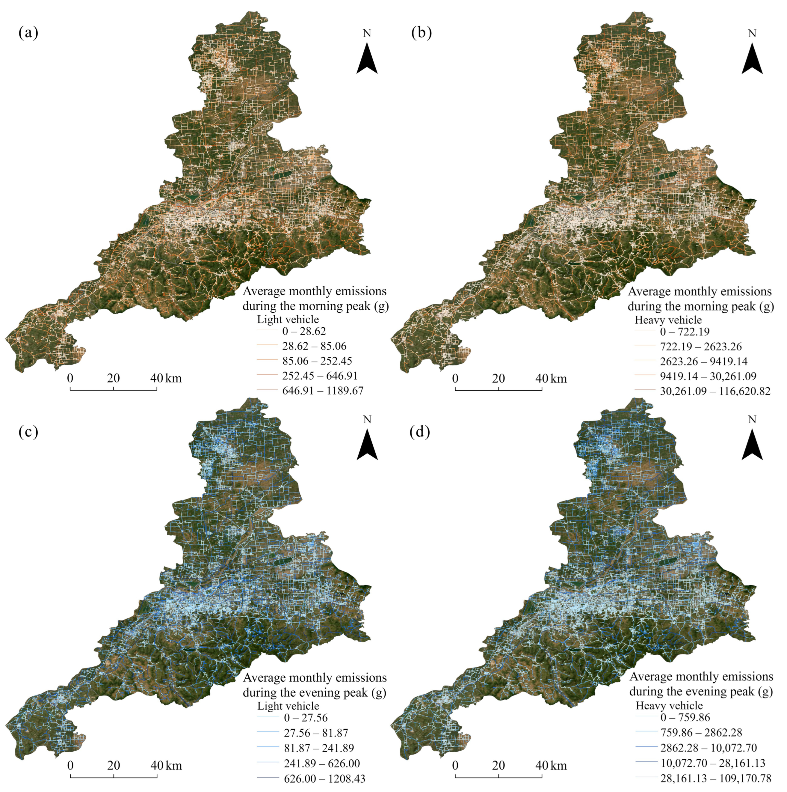
Figure A6 illustrates the spatial distribution of average monthly nitrogen oxide (NOX) emissions from light-duty and heavy-duty vehicles during the morning and evening peak periods in Jinan. During the morning peak, emissions from light-duty vehicles (Figure A6a) were relatively widespread but moderate in intensity. The highest emissions, ranging from 545.91 g to 1199.66 g, were concentrated in central urban areas and along major commuting corridors. In contrast, heavy-duty vehicle emissions (Figure A6b) during the same period were significantly higher and more spatially clustered. Emission hotspots appeared primarily along expressways and key freight routes, particularly in the southern and eastern parts of the city. Maximum values exceeded 17,662.81 g, indicating that heavy-duty traffic contributed substantially to morning NOX emissions. During the evening peak, emissions from light-duty vehicles (Figure A6c) showed a broader spatial distribution compared to the morning, with increased intensities both in urban centers and suburban peripheries. Peak values reached up to 1209.44 g, reflecting elevated usage of private vehicles during the evening commute. Heavy-duty vehicle emissions (Figure A6d) remained high, with values up to 19,097.78 g, and their spatial spread extended into industrial zones and logistics hubs. This suggested that freight transport activity continued actively into the evening hours.
Figure A7 showed the diurnal variation of NOX emissions from light and heavy vehicles in Jinan. Heavy vehicles consistently contributed the majority of emissions throughout the day. Their emissions began to rise sharply around 6:00, reaching a peak of approximately 210 g during the morning rush hour (7:00–9:00). Afterward, emissions slightly decreased but remained relatively high until the evening. Light vehicle emissions remained low and relatively stable across all hours, with only a slight increase during peak periods. The total emissions pattern closely followed that of heavy vehicles.
The annual NOX emissions from vehicles in Jinan were estimated to reach approximately 24,000 tons, which is higher than previous estimate of 18,600 tons based on statistic data in 2020 [29]. It is mainly because statistic data did not account for emissions from non-local transit vehicles, particularly trucks. This study uses dynamic data to capture this important emission contributor, 1.25 times higher when using high-resolution data compared to traditional aggregated estimates. Our results are consistent with those of Deng et al., showing that non-local trucks contribute 31% more pollution [10].
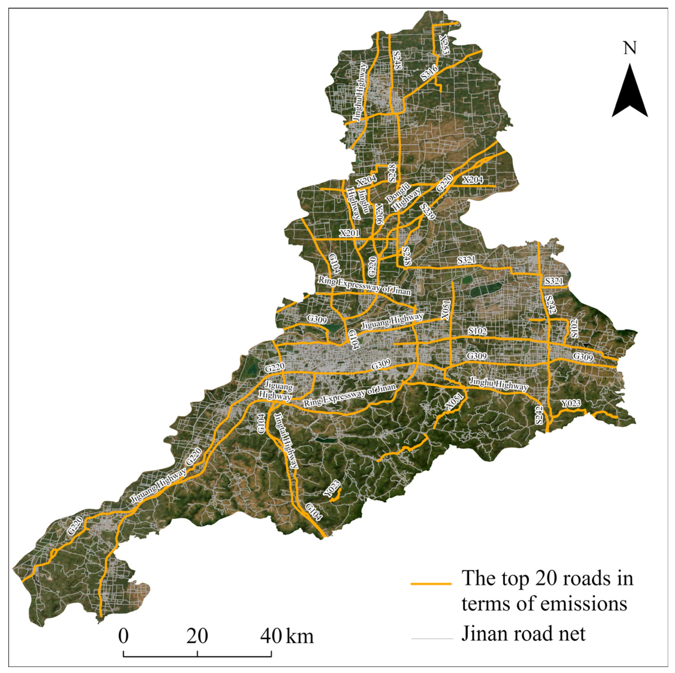
Annual NOX emissions are particularly prominent along major urban transportation routes such as the Jiguang Highway, G220 National Highway, and S248 Provincial Highway, driven by HDV fleets (Figure 6). In the southwestern part of Jinan City, Pingyin County stands out as a hotspot for pollution emissions, likely due to transit traffic along the Jiguang Expressway and G220 National Highway, as well as emissions associated with agricultural airport. The top 20 roads with the highest annualized pollution emissions are key arterial routes traversing the city both north–south and east–west, primarily consisting of national highways, provincial highways, and expressways (Table A7). The concentration of NOX emissions on the top 20 roads results mainly from several interconnected factors. These routes typically experience high volumes of heavy-duty vehicles. Traffic conditions often involve low and unstable speeds—such as congestion and stop-and-go flow—further increasing per-kilometer emissions. Additionally, the extended length and continuity of these roads accumulate substantial emissions. Finally, freight restrictions on expressways divert trucks to lower-class roads, intensifying local emissions. These findings revealed the spatial heterogeneity of vehicular NOX emissions and emphasized the dominant role of heavy-duty vehicles and lower-grade road types in regional air pollution in Jinan.

4. Discussion

4.1. Findings and Policy Recommendations

This study aims to develop a methodology that enables near real-time monitoring for urban vehicle emissions, with a high temporal (hourly) and spatial (road segment level) resolution. The method first establishes the digital twin GIS to accurately describe the road characteristics. Based on the GIS, we find a stable token data stream, i.e., the congestion index from the open-source map APP that could be accessed in a 15 min timespan. We then comply with data cleaning mechanisms and Random Forest algorithms to predict the vehicle emissions that cover the whole city with road segment granularity. The model training results are satisfactory both for the comparison of geographic distribution of vehicle emissions and for the trend and statistics of vehicle emissions at specific coordinates and timespans. The results enable accurate descriptions of environmental impacts, thus offering reliable data support for real-time control and management of vehicle emissions. Further, the aggregated results could be used to analyze the vehicle emission trend, thus helping with the development of mid- and long-term vehicle emissions control policy and low-emission zoning.
The proposed framework also has practical implications for near real-time urban management. First, by providing continuously updated traffic emission estimates, it could inform dynamic traffic control strategies, such as adjusting freight vehicle restrictions or deploying congestion mitigation measures at specific times of day. Second, integration with atmospheric dispersion models would enable short-term air quality nowcasting and forecasting, supporting proactive interventions to prevent pollution episodes. Third, the near real-time identification of high-emission corridors can provide actionable intelligence for enforcement, such as establishing checkpoints for heavy-duty vehicle inspections or expanding low-emission zones. Finally, this system could offer valuable decision support for both city-level strategic planning and neighborhood-scale interventions, making it directly relevant for policy implementation and urban governance.
The application of the modeling system in Jinan, a typical big Chinese city, shows a few interesting results. First, by using this completely bottom-up method, we found that the traditional top-down vehicle emission simulation models (vehicle population-based, fuel based, or total activity based) may underestimate vehicle emissions at the city level. This verifies a few scholars’ suspicions regarding incomplete representations in the traditional approach. The reasons are both that the pass-through vehicles are not captured in those top-down models, and that environment-damaging vehicle driving cycles are more commonly found in urban areas.
Township roads contribute the most to total nitrogen oxide emissions. This finding highlights an important policy implication: emission control strategies cannot focus solely on expressways or arterial roads. Township and county roads, which host significant freight activity at lower speeds, emerge as major emission hotspots. Targeted measures such as rerouting policies, speed management, or localized inspection checkpoints may therefore be more effective for reducing emissions in these areas.
The importance of heavy-duty vehicle emission control is further supported in this study. Despite accounting for about 20–30% of traffic flow, HDVs contribute to 70–80% of total vehicle emissions. More importantly, we found that HDV operation follows more regular routes and timing than passenger vehicles, and this high-resolution bottom-up method can effectively catch the operation characteristics of the trucks, thus offering opportunities in truck control. For example, the method could identify the key truck operational corridors with accurate location at a daily level, which gives the chance to control truck emissions through environmental enforcement, and warns the truck owner for traffic control and adjust dispatch operations. Furthermore, the results could also assist the electrification of HDVs by providing suggestions for planning and designing charging infrastructures.
Identifying the hotspots of the top 20 emission roads provides a clear pathway for policy action. Possible interventions include: (i) targeted roadside inspections and emission checks at key entry points to high-emission corridors to remove gross polluters; (ii) time-of-day restrictions or dynamic routing to shift freight movements away from sensitive periods or densely populated areas; (iii) speed management and signal-timing optimization to reduce stop-and-go conditions and lower per-kilometer emissions; (iv) prioritization of retrofitting, replacement, or electrification incentives for HDVs operating predominantly on hotspot corridors; and (v) structural interventions such as dedicated freight bypasses or improved pavement that reduce congestion and improve fuel economy.

4.2. Limitations

Despite the successes in simulating traffic flow in near real-time, there are still several shortfalls in the methodology that need further improvement. Firstly, congestion index alone cannot fully explain traffic volume due to its non-linear relationship with flow. For example, congestion index values of approximately 2.0 may correspond to different traffic volumes in the morning and evening peaks. To address this complexity, the Random Forest model leverages additional temporal predictors (hour of day, day of week, holiday indicators), which enable the model to distinguish such cases and improve predictive accuracy. Feature importance analysis confirms that congestion index and temporal variables are consistently among the top-ranked predictors, jointly accounting for most of the variance explained by the model.
A second limitation concerns the simplified classification of vehicles into only two categories: light-duty and heavy-duty vehicles. Due to current data restrictions, we were unable to obtain detailed vehicle information, including specific categories or usage purposes. As a result, the heterogeneous sub-groups within HDVs—such as buses, medium-duty delivery trucks, and long-haul freight trucks—were aggregated into a single category. This oversimplification may obscure distinct spatial and temporal emission patterns, and could introduce uncertainty in hotspot identification and trend analysis. Future work should aim to incorporate more refined classification when such data become available.
Furthermore, the cross-validation strategy adopted presents another methodological constraint. Although k-fold cross-validation is widely used for model evaluation, applying it directly to traffic flow data may lead to overly optimistic estimates of accuracy because of strong spatiotemporal autocorrelation. In particular, random splitting can assign highly correlated observations—such as consecutive hours on the same road segment, or adjacent road segments observed in the same hour—into both training and testing sets. This leakage of correlated samples reduces the independence of the validation process. While temporal cross-validation or spatial cross-validation would provide stricter and more realistic performance assessments, such approaches were not feasible in the present study due to data and sample size constraints. Future work should incorporate these validation designs to better quantify predictive uncertainty under realistic deployment conditions.
A further limitation of this study is that vehicle emission factors were modeled as a function of speed only, without explicitly accounting for other influencing variables such as ambient temperature, road topography, and vehicle load [30,31]. While these factors can significantly affect instantaneous emissions, the necessary high-resolution data were not available for Jinan, and systematic studies quantifying their effects remain relatively scarce. We acknowledge that this simplification may introduce biases in our inventory. Although our focus here is on mobile source NOX emissions, which are closely tied to vehicle operational states, integrating additional explanatory variables into emission factor models will be an important direction for future research.
Operational deployment remains a necessary step toward validating the proposed methodology within a real intelligent traffic management system. While designed for integration into such platforms, the framework has not yet been implemented or tested in a live operational environment in Jinan. Consequently, its practical efficiency, stability, and scalability under real-world conditions still require thorough evaluation.
It is also important to note that this study focused exclusively on the characterization of vehicle emissions and did not extend to assessing their impacts on ambient air quality and public health—outcomes that represent the ultimate purpose of emission control strategies. Future work should prioritize linking high-resolution emission estimates with air quality monitoring and health impact models. Our long-term goal is to develop an integrated big-data framework that holistically addresses traffic operations, emissions, environmental quality, and public health.

5. Conclusions

This study developed a high-resolution approach for traffic flow prediction and vehicle emission inventory construction by integrating multi-source geospatial data with machine learning techniques. We first built a comprehensive road network framework for Jinan City and employed a two-fold random forest model to predict hourly traffic flows. These predicted flows were then combined with speed-sensitive emission factors to estimate vehicle emissions at a high spatiotemporal resolution. In contrast to traditional static methods reliant on aggregated vehicle population data, our approach not only achieved significantly higher prediction accuracy but also captured transient and non-local emissions that are often missed in conventional inventories. Beyond its methodological advancements, the resulting high-resolution emission inventory offers actionable insights for refined urban governance. It can directly inform traffic management strategies, such as optimizing freight corridors, designating low-emission zones, and guiding infrastructure planning for vehicle electrification. Moreover, as the methodology depends on widely available multi-source traffic data, it is highly scalable and transferable to other Chinese cities and international contexts, thereby providing robust support for integrating traffic emission monitoring into sustainable air quality management and effective regulatory enforcement. This near real-time monitoring framework has the potential to serve not only as a research tool but also as an operational component of smart traffic and environmental management systems, providing a scientific basis for timely and targeted emission reduction policies.
The results demonstrated that temporal variables and the congestion index were the dominant factors influencing traffic flow and vehicle composition prediction. The Fold 1 model achieved strong accuracy under high traffic volume conditions, whereas the Fold 2 model showed systematic biases in freight-intensive periods, where it overestimated the passenger car share. Traffic analysis revealed a pronounced bimodal pattern for light-duty vehicle flows, with distinct morning and evening commuting peaks on ring expressways and highways, while heavy-duty vehicle flows remained relatively stable throughout the day, reflecting the effectiveness of time-based restriction policies. The study also found that heavy vehicle volumes were relatively higher on lower-grade roads, such as county and township roads, despite their limited traffic capacity. Emission estimates further indicated that heavy-duty vehicles, though accounting for a smaller share of total traffic, contributed highly to NOX emissions, with hotspots concentrated along expressways, ring roads, and major freight corridors. Township and county roads also emerged as important contributors due to heavy-duty vehicle freight activity, underscoring the spatial heterogeneity of urban emissions and the policy-driven routing of heavy vehicles toward peripheral areas. These findings underscore the spatial heterogeneity of NOX pollution and highlight the dominant contribution of heavy-duty vehicles and lower-grade roads to regional air pollution. Furthermore, the high-resolution traffic emission inventory developed in this study can be integrated with chemical transport models (e.g., WRF-Chem) to generate dynamic air quality profiles and forecasts, thereby directly linking emission estimates with exposure assessment and policy evaluation.

Author Contributions

Conceptualization, X.Y., C.H. and Q.Y.; methodology, X.Y., C.H. and Z.C.; validation, X.Y., Z.C. and X.Z.; formal analysis, X.Y. and Q.Y.; investigation, H.W. and D.H.; resources, X.Y.; data curation, X.Y. and Z.C.; writing—original draft preparation, X.Y., D.H. and J.F.; writing—review and editing, C.H.; visualization, J.F., C.Z. and P.W.; supervision, C.H. and D.H. All authors have read and agreed to the published version of the manuscript.

Funding

This research was funded by Energy Foundation China, grant number G-1809-28502.

Institutional Review Board Statement

Not applicable.

Informed Consent Statement

Informed consent was obtained from all subjects involved in the study.

Data Availability Statement

The road network data were obtained from OpenStreetMap and NavInfo and are publicly available online. Baidu congestion index data are accessible through the Baidu Map platform. Emission factor data were compiled from laboratory tests and on-road measurements reported by the Vehicle Emission Control Center (VECC) and related studies (see Appendix A.5 and cited references). Traffic flow observations and automated license plate recognition (ALPR) outputs were provided by the Jinan Municipal Transportation authorities under a data-sharing agreement. Due to privacy regulations, the raw ALPR database containing license plate numbers cannot be made publicly available. This study only used anonymized and aggregated outputs (traffic counts, turning movements, and vehicle-classification results) supplied by the authorities. Researchers interested in accessing these data may contact the Jinan Municipal Transportation authorities, subject to approval and data-sharing agreements.

Conflicts of Interest

Author Xuejun Yan, Qi Yang, Jingyang Fan, Ziyuan Cai, Pan Wang, Xiuli Zhang, Hengzhi Wang, Chenxi Zhu and Dongquan Hewas employed by the company Beijing Smart Green Transport Research Centre. The remaining authors declare that the research was conducted in the absence of any commercial or financial relationships that could be construed as a potential conflict of interest.

Abbreviations

The following abbreviations are used in this manuscript:
LDVslight-duty vehicles
HDVsheavy-duty vehicles
OBDOn-Board Diagnostics
RFRandom Forest
PCEsPassenger Car Equivalents

Appendix A

Appendix A.1. Road Characteristic Data

To comprehensively analyze urban traffic dynamics, we developed a static road network dataset that integrates various spatial and infrastructural attributes. We extracted road characteristic data—including road width, number of lanes, and road classification—from street-view imagery and assigned them to a simplified single-line road network. Using land use data for the city of Jinan, we examined how urban infrastructure and spatial development patterns influence traffic behavior. We also incorporated population density data to assess spatial variations in traffic volume and distribution. Furthermore, we identified points of interest (POIs), such as hospitals, schools, marketplaces, banks, and tourist attractions, using data from Amap (Gaode Maps) to evaluate their effects on local traffic flow. These components collectively constitute a static dataset based on the road network. In addition to assigning road attributes and integrating traffic volume data, we conducted preprocessing of congestion and POI data within a Geographic Information System (GIS) environment to support in-depth road network analysis. We first transformed polyline-based congestion index data into point features centered along each road segment through a line-to-point conversion. Then, we spatially joined these point-based congestion values to the single-line road network using an empirically determined 15 m search radius. For each road segment, we averaged the matched congestion points to derive a representative congestion index. To assess the influence of surrounding land use on traffic patterns, we applied buffer analysis to count the number of POIs within specific distances from each road segment—for example, educational facilities within 50 m, commercial centers within 100 m, and financial institutions within 300 m. We also computed the shortest distance from each road segment to the nearest POI of each category to construct a spatial profile of accessibility and land use intensity.

Appendix A.2. Preprocessing of Road Network

In this study, the road segment—defined as the stretch of roadway between two consecutive intersections or highway ramps—served as the basic unit for traffic speed evaluation. The road network dataset for Jinan comprises 13,519 road segments, covering the entire urban area with a cumulative road length of approximately 9935.3 km. Develop single-line road network in GIS. We obtained the Jinan Road network information is based on an integration of OpenStreetMap and NavInfo data sources, the system includes information of road width, number of lanes, and road classification. The road classification is divided into eight categories: Level 9 roads, township roads, county roads, national roads, provincial roads, pedestrian roads, urban expressways, and highways. Road width is measured in meters, and the number of lanes is expressed as a count. During preprocessing, duplicate or fragmented road segments were merged, and topological integrity was checked to avoid discontinuities in the simplified single-line network. We first restructured Jinan Road network into a simple-line structure in GIS to simplified calculation. The work involves (1) merging the lanes of the road and make road lane numbers as the attribution; (2) assigning each road segment (road between two intersections) with an id number for future data coordination; and (3) for complete road environment such as overpass and auxiliary roads, we simply merge all the lines together.

Appendix A.3. Matching Congestion Index to Roads

Assign the congestion index to each identified road segment. We applied a length-weighted averaging method to minimize biases due to differences in segmentation definitions across data sources, and extreme outlier values were removed before averaging. The work involves two steps; step one is to match the Baidu Road network with the simple-line road network we have developed in GIS; the second step is to average the congestion index into one number for each road segment at each hour. As the method in dividing road segments in two road networks are different, we have to combine a few congestions index in one identified single-lined road segment, we simply using a length-weight segment average approach to obtain one congestion index number for certain road segment (Figure A1).
Figure A1. Diagram of assigning values to road congestion index.
Atmosphere 16 01213 g0a1
C o n g e s t i o n   i n d e x   f o r   R S i   a t   c e r t a i n   h o u r = i j × l j l j
where  R S i  represents the i-th road section (or road segment) under consideration;  i j  represents the congestion index of the j-th sub segment within a specific time period of the road section; and  l j  represents the length of the j-th sub segment.

Appendix A.4. Building a Traffic Flow Simulation Training Dataset

To construct the training dataset for traffic flow simulation, we treated all preceding variables—such as congestion indices, road attributes, and temporal indicators—as input features (X), and used observed hourly traffic volume data as the target variable (y). We sourced congestion index data from Baidu Maps due to its accessibility and temporal stability, which addressed concerns regarding data availability and consistency. These data span three representative time periods: November 2020, and March and July 2021. The congestion index ranges from 1 (indicating free-flowing traffic) to 18 (indicating severe congestion) and was recorded at hourly intervals across the entire Jinan metropolitan area.
We obtained traffic flow data from the Jinan Municipal Transportation Bureau, which monitors vehicular flow at over 800 key intersections throughout the city. To ensure data usability, abnormal or missing records from traffic surveillance cameras were rigorously screened. Periods impacted by equipment malfunction, signal loss, or incomplete video recognition were excluded from the dataset, ensuring that only validated traffic counts were retained for training and that the simulation was based on reliable, consistent observations.
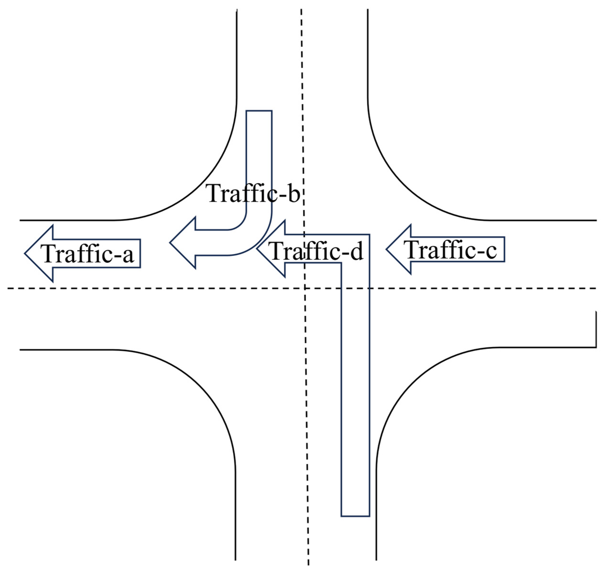
To convert intersection-level camera observations into directional road-segment flows, we applied the following procedure: (i) Aggregate hourly traffic counts from each surveillance camera at the intersection. (ii) Assign these approach counts to outgoing road segments according to the monitored turning directions. (iii) Compute the directional flow for each road segment by summing the contributions from connected approaches. For example, as illustrated in Figure A2, the traffic volume of segment a is obtained as Traffic-a = Traffic-b + Traffic-c + Traffic-d. (iv) The resulting segment-level directional flows were compiled to form the training dataset for the Random Forest model. This procedure ensures that camera observations at intersections are consistently translated into road-segment flows in the simplified network.
Most surveillance cameras are concentrated in central urban areas, with supplementary coverage along major highway corridors. We mapped this camera-derived traffic data to corresponding primary road segments by leveraging information from neighboring intersections to collaboratively estimate traffic volumes along each segment of the single-line road network, which served as the training set for the machine learning model. The traffic police department provided surveillance data, captured by cameras positioned at critical intersections. Typically, each intersection is equipped with two cameras—one monitoring the east–west direction and the other monitoring the north–south direction. In cases where only one camera is present, it monitors traffic in a single direction. Some cameras record only one side of the road, while others capture both sides. For road segments covered by dual-side cameras, we aggregated the flow data from both sides into a single directional traffic volume, ensuring consistent input for model training. This configuration enabled comprehensive spatial and directional coverage, reliably capturing vehicle movements at each monitored intersection.
A significant challenge in the data preparation process involved converting intersection-level camera observations into segment-level traffic flow values required for fine-grained simulation and training. Each intersection, equipped with up to four directional cameras, generated time-stamped vehicle detection records. We aggregated these records and mapped them to corresponding road segments using a schematic diagram developed by the research team. This diagram helped us track vehicle trajectories and estimate directional traffic volumes by accounting for turning movements and exit flows from intersections. As a result, we achieved an accurate and segment-specific assignment of traffic volume data, suitable for training data-driven traffic flow simulation models. Finaly, we used automated license plate recognition (ALPR) systems to identify light-duty vehicles (LDVs) and heavy-duty vehicles (HDVs) based on plate number patterns and vehicle registration information. This classification was based on recognized plate patterns and category information from aggregated registration records supplied by the Jinan Municipal Transportation authorities. To comply with privacy regulations, raw license plate data were not used; instead, only anonymized and aggregated vehicle-class information was provided for analysis.
Figure A2. Assignment of Traffic Flow Data to Simplified Road Network.
Atmosphere 16 01213 g0a2
Traffic-a = Traffic-b + Traffic-c + Traffic-d
where Traffic-a denotes the total observed traffic flow exiting the western approach (left arm) of the intersection. Traffic-b, Traffic-c, and Traffic-d represent incoming flows from the other three approaches (north, east, and south, respectively) that eventually turn left, go straight, or turn right into the westbound segment.

Appendix A.5. Dynamic Emissions Factor Data

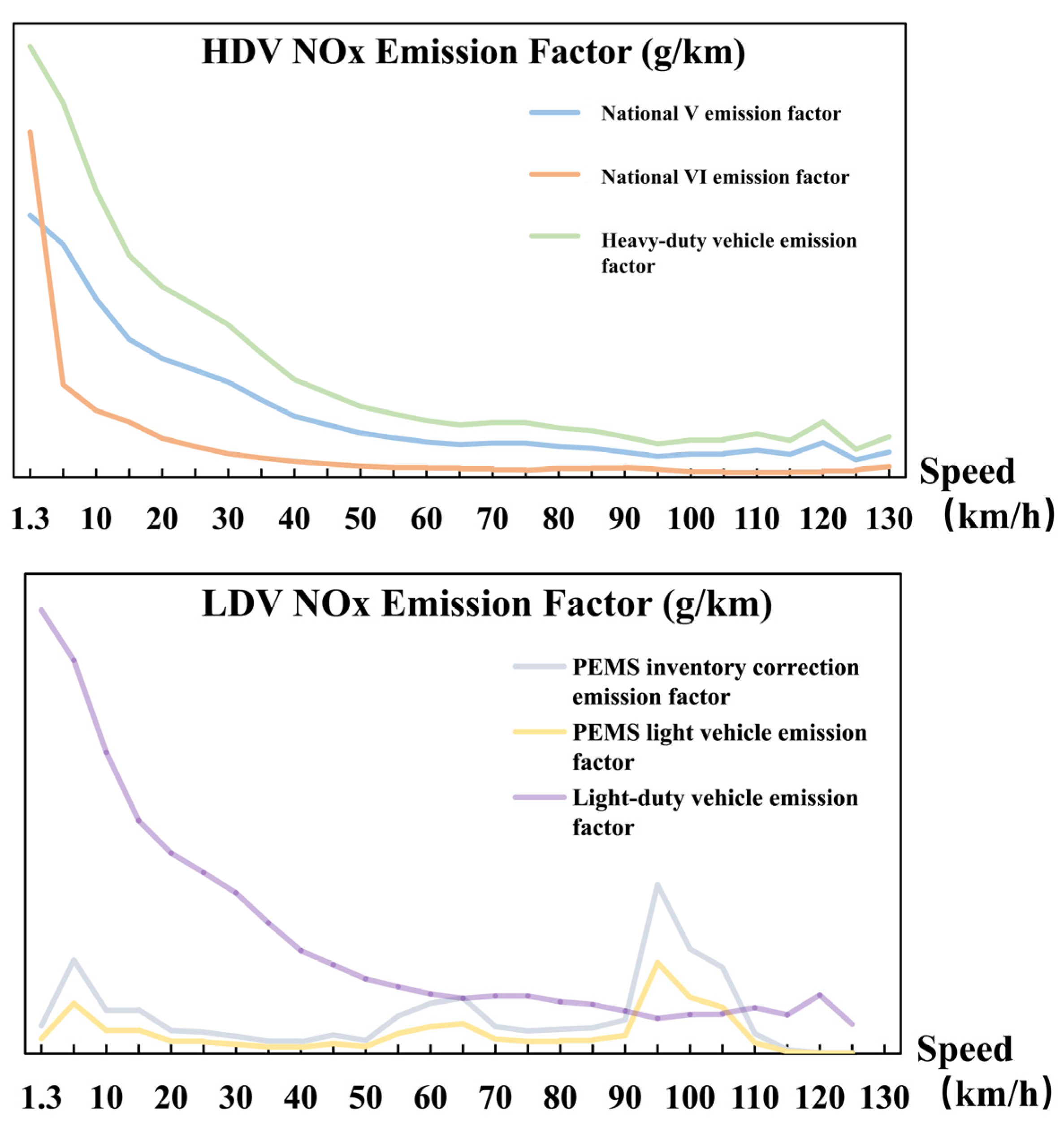
Speed-dependent emission factors (EFs) for light-duty (LDVs) and heavy-duty vehicles (HDVs) were compiled from laboratory chassis dynamometer tests conducted at the Vehicle Emission Control Center (VECC) and from on-road measurements using Portable Emission Measurement Systems (PEMSs) and On-Board Diagnostics (OBD). For each vehicle class, raw EF measurements were grouped by mean driving speed intervals (e.g., 0–10, 10–20, … km/h). Within each speed bin, the sample mean and standard deviation were computed. The resulting EF-speed relationships are illustrated in Appendix A Figure A3. This approach is well-justified, as vehicle speed is a well-established critical factor influencing vehicle emission factors [32].
By harmonizing PEMS- and OBD-derived emission factors with local driving cycles and official Jinan fleet data, we ensured the robustness of the emission dataset through its alignment with both empirical measurements and authoritative statistics. We derived dynamic emission factor data from real-world vehicle testing using PEMS for LDVs and OBD systems for HDVs. To ensure alignment with local conditions, we modified the raw data to reflect actual driving cycles observed in Jinan. To account comprehensively for different vehicle types, fuel types, and emission standards, we calculated weighting factors for HDV and LDV emission estimations based on the current composition of the vehicle fleet in Jinan. The Jinan Environmental Protection Bureau and the Jinan Municipal Transportation Bureau provided these fleet composition data.
For consistency with the vehicle classification scheme used in the traffic flow analysis, we categorized taxis, private cars, micro and small passenger vehicles, and micro and light trucks as LDVs. In contrast, we classified buses, medium and large passenger vehicles, and medium and heavy trucks as HDVs. By applying population-based weighting factors across these vehicle categories, we constructed speed-dependent emission factor curves for both LDVs and HDVs. These curves incorporate the distribution of vehicle types and actual operating conditions, thereby capturing the spatial and temporal variability of emissions under real-world traffic scenarios. Figure A3 illustrates the resulting emission factor curves, which serve as a key input for dynamic emission modeling.
Figure A3. HDV and LDV NOX Emission Factors Associated with driving speed.
Atmosphere 16 01213 g0a3
Lastly, speed-specific vehicle emission factors, derived from laboratory tests conducted by the VECC, were incorporated to support emissions analysis in relation to traffic patterns. These emission factors, obtained through controlled laboratory conditions, provided essential data for modeling the emissions of various vehicle types under different driving speeds. To enhance the accuracy of the emission estimates, data from the PEMS were also integrated. PEMS provided real-world, on-road emission data, allowing for a more precise calibration of the model in terms of actual driving conditions. The combination of VECC’s laboratory-based emission factors and PEMS data ensured a comprehensive analysis of vehicle emissions, accounting for both controlled and real-world driving scenarios. These factors were crucial for understanding the dynamic relationship between traffic flow, vehicle activity, and emission levels, ultimately improving the overall estimation of air pollution in urban environments.
Table A1. Example of Data Section-Congestion Index.
ObjectiveYearMonthDayHourCongWeekday
1202091010
220209211.050151
320209321.057552
420209431.069153
520209541.084054
………………………………5
14572020930231.047956
Table A2. Example of Data Section-Road attributes.
Featured_RoadWidthNumber of Lanes, Category
featured_road415FID
featured_road59.6Shape
………………
featured_road66.3Office-50m
Table A3. Example of Data Section-Road environment attributes.
Trans_50mResta_50mOffic_50mMall_50mHotel_50m
00000
11111
Table A4. Example of Data Section-Traffic volume.
Checkpoint DirectionObjectiveAnalysis TimeTraffic Flow
East–West Direction19605 September 2020 00:00 5 September 2020 01:0015
East–West Direction38541 September 2020 00:00 1 September 2020 01:0027
……………………
North–South Direction57111 September 2020 05:00 1 September 2020 06:0010
North–South Direction13,5161 September 2020 00:00 1 September 2020 01:0050
…………
Table A5. Example of Data Section-The number of vehicles for each vehicle type.
Small Car License PlateLarge Car License PlateOther License Plates
14380
9242
783
19147
………………
405891
Table A6. Data type and data sources.
Data TypeSelected DataData SourcePreprocessing MethodNotes
Congestion Index Baidu MapArcGIS 10.8 software preprocessingNovember 2020, March 2021, July 2021
Road attributesWidth, number of lanes, categoryPurchased The number of lanes is an estimate obtained through visual algorithm analysis of street view image data.
Road environment attributesTraffic, office, shopping mall, education, bank, tourist attraction, etc.AmapArcGIS 10.8 buffer analysisSeptember 2020
Distance from the center of the road to important urban facilitiesAmapArcGIS 10.8 distance calculationSeptember 2020
Population density in the surrounding areaWorldPop projectArcGIS 10.8 buffer zone analysisSeptember 2020
Surrounding land use classification10 m resolution global land use classification raster data released by the Department of Earth System Science at Tsinghua University in 2017The area of these land types within a certain distance from the road was calculated through ArcGIS 10.8 buffer zone analysis and overlay analysis.September 2020
Traffic volumeTraffic monitor cameras dataJinan Municipal Transportation BureauSpatial positioningSeptember 2020
The number of vehicles for each vehicle typeVehicle registration dataJinan Municipal Transportation Bureau
Jinan Environmental Protection Bureau
Table A7. Emission inventories of top emission roads.
NameEmissions of Light Vehicles (g)Emissions of Heavy Vehicles (g)Total Emissions (g)
G104811,725.865917,777,647.0118,589,372.87
G2201,053,022.9873,938,909.0274,991,932
G309614,772.33468,951,101.2699,565,873.603
S102667,393.30811,288,846.5611,956,239.87
S239154,393.846110,549,275.4510,703,669.3
S242487,171.154211,889,482.7612,376,653.91
S248379,582.065143,798,521.7844,178,103.84
S316239,187.94428,473,821.0798,713,009.023
S321178,110.870313,538,434.2213,716,545.09
X051582,188.44239,660,950.01310,243,138.46
X201124,852.13886,979,132.567,103,984.699
X204214,828.34158,251,207.3378,466,035.678
X206199,439.03788,147,492.2718,346,931.309
X253146,818.61478,350,798.8978,497,617.512
Y023384,591.11289,673,257.2310,057,848.34
Donglü Highway291,043.226411,194,122.5911,485,165.81
Jiguang Highway1,137,262.19315,801,465.2316,938,727.42
Jinghu Highway736,899.812522,875,976.2123,612,876.02
Jingtai Highway650,422.3659,812,123.1610,462,545.52
Ring Expressway of Jinan859,408.911917,586,604.5318,446,013.44

Appendix B

Figure A4. Traffic Flow by Vehicle Aggregated by Week. (a) daily traffic flow of light vehicles; (b) daily traffic flow of heavy vehicles; (c) proportion of daily traffic flow for light vehicles (orange) and heavy vehicles (blue) over one week.
Atmosphere 16 01213 g0a4
Figure A5. Proportion of light and heavy vehicles of different road types.
Atmosphere 16 01213 g0a5
Figure A6. Spatial distribution of average monthly NOX emissions from light-duty and heavy-duty vehicles during morning and evening peak hours in Jinan. (a) Light-duty vehicles, morning peak; (b) heavy-duty vehicles, morning peak; (c) light-duty vehicles, evening peak; (d) heavy-duty vehicles, evening peak.
Atmosphere 16 01213 g0a6
Figure A7. Hourly Distribution of Average Monthly NOX Emissions from Light and Heavy-Duty Vehicles in Jinan.
Atmosphere 16 01213 g0a7

References

  1. Zhou, Q.; Yun, J.; Li, X.; Zhang, X.; Liu, B.; Zhang, S.; Zheng, X.; Yue, W.; Li, X.; Zhang, W. Vehicle Emissions in a Megacity of Xi’an in China: A Comprehensive Inventory, Air Quality Impact, and Policy Recommendation. Urban Clim. 2023, 52, 101740. [Google Scholar] [CrossRef]
  2. Li, H.; Zheng, B.; Lei, Y.; Hauglustaine, D.; Chen, C.; Lin, X.; Zhang, Y.; Zhang, Q.; He, K. Trends and Drivers of Anthropogenic NOx Emissions in China since 2020. Environ. Sci. Ecotechnol. 2024, 21, 100425. [Google Scholar] [CrossRef]
  3. Heydari, S.; Tainio, M.; Woodcock, J.; de Nazelle, A. Estimating Traffic Contribution to Particulate Matter Concentration in Urban Areas Using a Multilevel Bayesian Meta-Regression Approach. Environ. Int. 2020, 141, 105800. [Google Scholar] [CrossRef]
  4. Guo, H. Review the Evolution of Chinese Legislation on Air Pollution Prevention and Control. Int. J. Nat. Resour. Ecol. Manag. 2020, 5, 49. [Google Scholar] [CrossRef]
  5. Yu, Y.; Dai, C.; Wei, Y.; Ren, H.; Zhou, J. Air Pollution Prevention and Control Action Plan Substantially Reduced PM2.5 Concentration in China. Energy Econ. 2022, 113, 106206. [Google Scholar] [CrossRef]
  6. Mak, H.W.; Ng, D.C. Spatial and socio-classification of traffic pollutant emissions and associated mortality rates in high-density Hong Kong via improved data analytic approaches. Int. J. Environ. Res. Public Health 2021, 18, 6532. [Google Scholar] [CrossRef]
  7. Zhang, K.; Batterman, S. Air pollution and health risks due to vehicle traffic. Sci. Total Environ. 2013, 450, 307–316. [Google Scholar] [CrossRef] [PubMed]
  8. Wang, H.; Chen, C.; Huang, C.; Fu, L. On-Road Vehicle Emission Inventory and Its Uncertainty Analysis for Shanghai, China. Sci. Total Environ. 2008, 398, 60–67. [Google Scholar] [CrossRef]
  9. Tripp-Barba, C.; Barbecho, P.; Urquiza, L.; Aguilar-Calderón, J.A. A Comparison of Vehicle Emissions Control Strategies for Smart Cities. PeerJ Comput. Sci. 2023, 9, e1676. [Google Scholar] [CrossRef]
  10. Deng, F.; Lv, Z.; Qi, L.; Wang, X.; Shi, M.; Liu, H. A Big Data Approach to Improving the Vehicle Emission Inventory in China. Nat. Commun. 2020, 11, 2801. [Google Scholar] [CrossRef] [PubMed]
  11. Kousoulidou, M.; Fontaras, G.; Ntziachristos, L.; Bonnel, P.; Samaras, Z.; Dilara, P. Use of Portable Emissions Measurement System (PEMS) for the Development and Validation of Passenger Car Emission Factors. Atmos. Environ. 2013, 64, 329–338. [Google Scholar] [CrossRef]
  12. Jiang, L.; Xia, Y.; Wang, L.; Chen, X.; Ye, J.; Hou, T.; Wang, L.; Zhang, Y.; Li, M.; Li, Z.; et al. Hyperfine-Resolution Mapping of on-Road Vehicle Emissions with Comprehensive Traffic Monitoring and an Intelligent Transportation System. Atmos. Chem. Phys. 2021, 21, 16985–17002. [Google Scholar] [CrossRef]
  13. Zhang, S.; Niu, T.; Wu, Y.; Zhang, K.M.; Wallington, T.J.; Xie, Q.; Wu, X.; Xu, H. Fine-Grained Vehicle Emission Management Using Intelligent Transportation System Data. Environ. Pollut. 2018, 241, 1027–1037. [Google Scholar] [CrossRef] [PubMed]
  14. Nyhan, M.; Sobolevsky, S.; Kang, C.; Robinson, P.; Corti, A.; Szell, M.; Streets, D.; Lu, Z.; Britter, R.; Barrett, S.R.H.; et al. Predicting Vehicular Emissions in High Spatial Resolution Using Pervasively Measured Transportation Data and Microscopic Emissions Model. Atmos. Environ. 2016, 140, 352–363. [Google Scholar] [CrossRef]
  15. Alam, G.M.I.; Arfin Tanim, S.; Sarker, S.K.; Watanobe, Y.; Islam, R.; Mridha, M.F.; Nur, K. Deep Learning Model Based Prediction of Vehicle CO2 Emissions with eXplainable AI Integration for Sustainable Environment. Sci. Rep. 2025, 15, 3655. [Google Scholar] [CrossRef]
  16. Li, J.; Jiang, C.; Han, K.; Yu, Q.; Zhang, H. High-Resolution Spatiotemporal Inference of Urban Road Traffic Emissions Using Taxi GPS and Multi-Source Urban Features Data: A Case Study in Chengdu, China. Urban Inform. 2024, 3, 17. [Google Scholar] [CrossRef]
  17. Yang, J.; Wen, Y.; Wang, Y.; Zhang, S.; Pinto, J.P.; Pennington, E.A.; Wang, Z.; Wu, Y.; Sander, S.P.; Jiang, J.H.; et al. From COVID-19 to Future Electrification: Assessing Traffic Impacts on Air Quality by a Machine-Learning Model. Proc. Natl. Acad. Sci. USA 2021, 118, e2102705118. [Google Scholar] [CrossRef] [PubMed]
  18. Moslehi, M.M. Exploring Coverage and Security Challenges in Wireless Sensor Networks: A Survey. Comput. Netw. 2025, 260, 111096. [Google Scholar] [CrossRef]
  19. Hariri, R.H.; Fredericks, E.M.; Bowers, K.M. Uncertainty in Big Data Analytics: Survey, Opportunities, and Challenges. J. Big Data 2019, 6, 44. [Google Scholar] [CrossRef]
  20. Sabet, S.; Farooq, B. Exploring the Combined Effects of Major Fuel Technologies, Eco-Routing, and Eco-Driving for Sustainable Traffic Decarbonization in Downtown Toronto. Transp. Res. Part A Policy Pract. 2025, 192, 104385. [Google Scholar] [CrossRef]
  21. Ren, C.; Fu, F.; Yin, C.; Lu, L.; Cheng, L. A Combined Model for Short-Term Traffic Flow Prediction Based on Variational Modal Decomposition and Deep Learning. Sci. Rep. 2025, 15, 17142. [Google Scholar] [CrossRef]
  22. Chang, V.; Xu, Q.A.; Hall, K.; Oluwaseyi, O.T.; Luo, J. Comprehensive analysis of UK AADF traffic dataset set within four geographical regions of England. Expert Syst. 2023, 40, e13415. [Google Scholar] [CrossRef]
  23. Hassan, H.M.; Abdel-Aty, M.A. Predicting reduced visibility related crashes on freeways using real-time traffic flow data. J. Saf. Res. 2013, 45, 29–36. [Google Scholar] [CrossRef]
  24. Liu, D.; An, C.; Yasir, M.; Lu, J.; Xia, J. A machine learning based method for real-time queue length estimation using license plate recognition and GPS trajectory data. KSCE J. Civ. Eng. 2022, 26, 2408–2419. [Google Scholar] [CrossRef]
  25. Wu, X.; Huang, H.; Zhou, T.; Tian, Y.; Wang, S.; Wang, J. An Urban Road Traffic Flow Prediction Method Based on Multi-Information Fusion. Sci. Rep. 2025, 15, 5568. [Google Scholar] [CrossRef]
  26. Kong, X.; Xu, Z.; Shen, G.; Wang, J.; Yang, Q.; Zhang, B. Urban traffic congestion estimation and prediction based on floating car trajectory data. Future Gener. Comput. Syst. 2016, 61, 97–107. [Google Scholar] [CrossRef]
  27. Wang, J.; Wang, R.; Yin, H.; Wang, Y.; Wang, H.; He, C.; Liang, J.; He, D.; Yin, H.; He, K. Assessing Heavy-Duty Vehicles (HDVs) on-Road NOx Emission in China from on-Board Diagnostics (OBD) Remote Report Data. Sci. Total Environ. 2022, 846, 157209. [Google Scholar] [CrossRef]
  28. Guo, M.; Ning, M.; Sun, S.; Xu, C.; Zhang, G.; Zhang, L.; Zhang, R.; Zheng, J.; Chen, C.; Jia, Z.; et al. Estimation and analysis of air pollutant emissions from on-road vehicles in Changzhou, China. Atmosphere 2024, 15, 192. [Google Scholar] [CrossRef]
  29. Wen, Y.; Liu, M.; Zhang, S.; Wu, X.; Wu, Y.; Hao, J. Updating on-road vehicle emissions for China: Spatial patterns, temporal trends, and mitigation drivers. Environ. Sci. Technol. 2023, 57, 14299–14309. [Google Scholar] [CrossRef]
  30. Zhang, M.; Wang, S.; Yu, W.; Tao, C.; Zhu, S.; Ma, J.; Wang, P.; Zhang, H. The major role of anthropogenic emission underestimation in PM2. 5 estimation uncertainty over the Tibetan Plateau. Geophys. Res. Lett. 2025, 52, e2024GL110513. [Google Scholar] [CrossRef]
  31. Qian, H.; Yuan, Z.; Chen, N.; Zhu, X.; Huang, S.; Lu, C.; Liu, K.; Zhou, F.; Smith, P.; Tian, H.; et al. Legacy effects cause systematic underestimation of N2O emission factors. Nat. Commun. 2025, 16, 2775. [Google Scholar] [CrossRef] [PubMed]
  32. Pandian, S.; Gokhale, S.; Ghoshal, A.K. Evaluating effects of traffic and vehicle characteristics on vehicular emissions near traffic intersections. Transp. Res. Part D Transp. Environ. 2009, 14, 180–196. [Google Scholar] [CrossRef]
Figure 1. Diagram of modeling flow of traffic prediction and emission estimations.
Atmosphere 16 01213 g001
Figure 2. Model results for PCE and car type ratio. (a) Comparison between actual and predicted PCE/h with regression fit. (b) Importance of input variables used in the PCE prediction model. (c) Scatterplot of actual versus predicted car type ratio with regression line. (d) Relative importance of variables used in the car type ratio prediction model.
Atmosphere 16 01213 g002
Figure 3. Spatial and temporal patterns of different motor vehicle traffic volume in Jinan City. (ac) Spatial distribution of traffic volumes on the Jinan road network: (a) light vehicles, (b) heavy vehicles, and (c) total traffic. (di) Diurnal variations of light vehicle (orange line) and heavy vehicle (blue line) traffic flows on different road types: (d) Urban Ring Expressway, (e) Highway, (f) National Road, (g) Provincial Road, (h) County Road, and (i) Township Road.
Atmosphere 16 01213 g003
Figure 4. Spatial distribution of NOX emissions from different vehicle types in Jinan on road networks and spatial grids. (ac) NOX emissions from: (a) light vehicles, (b) heavy vehicles, and (c) all vehicles on the Jinan road network; (df) Spatial distribution of NOX emissions in Jinan: (d) light vehicles, (e) heavy vehicles, and (f) all vehicles.
Atmosphere 16 01213 g004
Figure 5. NOX emissions from light and heavy vehicles in Jinan by road types.
Atmosphere 16 01213 g005
Figure 6. The top twenty roads in Jinan with the highest annualized total pollutant emissions.
Atmosphere 16 01213 g006
Disclaimer/Publisher’s Note: The statements, opinions and data contained in all publications are solely those of the individual author(s) and contributor(s) and not of MDPI and/or the editor(s). MDPI and/or the editor(s) disclaim responsibility for any injury to people or property resulting from any ideas, methods, instructions or products referred to in the content.