Article

Evaluation and Projection of Degree-Days and Degree-Days Categories in Southeast Europe Using EURO-CORDEX

National Institute of Meteorology and Hydrology, 66, Tsarigradsko Shose Blvd, 1784 Sofia, Bulgaria
*
Author to whom correspondence should be addressed.
Atmosphere 2025, 16(10), 1153; https://doi.org/10.3390/atmos16101153
Submission received: 18 August 2025 / Revised: 26 September 2025 / Accepted: 26 September 2025 / Published: 1 October 2025
(This article belongs to the Section Climatology)

Abstract

The temperature-based indicators heating and cooling degree days, are frequently utilized to quantitatively link indoor energy demand and outdoor thermal conditions, especially in the context of climate change. We present a comprehensive study of the heating and cooling degree-days and the degree-days categories for the near past (1976–2005), and the AR5 RCP4.5 and RCP8.5 scenario-driven future (2066–2095) over Southeast Europe based on an elaborated methodology and performed using a 19 combinations of driving global and regional climate models from EURO-CORDEX with horizontal resolution of 0.11°. Alongside the explicit focus of the degree-days categories and the finer grid resolution, the study benefits substantially from the consideration of the monthly, rather than annual, time scale, which allows the assessment of the intra-annual variations of all analyzed parameters. We provide evidences that the EURO-CORDEX ensemble is capable of simulating the spatiotemporal patterns of the degree-days and degree-day categories for the near past period. Generally, we demonstrate also a steady growth in cooling and a decrease in heating degree-days, where the change of the former is larger in relative terms. Additionally, we show an overall shift toward warmer degree-day categories as well as prolongation of the cooling season and shortening of the heating season. As a whole, the magnitude of the projected long-term changes is significantly stronger for the ’pessimistic’ scenario RCP8.5 than the ’realistic’ scenario RCP4.5. These outcomes are consistent with the well-documented general temperature trend in the gradually warming climate of Southeast Europe. The patterns of the projected long-term changes, however, exhibit essential heterogeneity, both in time and space, as well as among the analyzed parameters. This finding is manifested, in particular, in the coexistence of opposite tendencies for some degree-day categories over neighboring parts of the domain and non-negligible month-to-month variations. Most importantly, the present study unequivocally affirms the significance of the anticipated long-term changes of the considered parameters over Southeast Europe in the RCP scenario-driven future with all subsequent and far-reaching effects on the heating, cooling, and ventilation industry.

1. Introduction

It is widely accepted today that shifting weather patterns and climatic conditions threaten human health and the planet’s. The IPCC-AR6 Synthesis Report [1] states that there is no doubt that human activity has played a role in global warming, mainly through the emission of greenhouse gases (GHG). With numerous climate-related hazards and an increase in the frequency and duration of extreme weather events, the region around the Mediterranean basin, which includes Southeast Europe (SEEu), is widely regarded as being among the most vulnerable to climate change [2,3,4,5]. Alongside to a number of other hazards, industries such as the heating, ventilation, and air-conditioning (HVAC) sector are both directly and indirectly impacted by climate change. About one-third of all energy use worldwide is attributed to household use [6], with HVAC systems using a significant amount of that portion [7]. Globally, buildings also contribute more than 30% of global annual carbon dioxide emissions [5]. This energy demand directly affects the consumption of electricity and fossil fuels, as well as the load on the electrical grid. The energy consumption of HVAC in enclosed spaces is primarily attributed to outdoor temperature conditions. There are additional factors that could be addressed, such as wind speed, cloud cover, humidity, and snow cover. Numerous underlying drivers, including solar irradiation, building aspect, window size, ventilation behavior, occupancy and heating patterns, and more, have a significant impact on these factors. However, it should be underscored that all these factors are sources of additional uncertainty and introduce more complexity in the analysis. Similarly to most recent studies sharing the same methodological framework, they are left outside the scope of this work [8]. Numerous recent studies [9,10,11,12,13] addressed the meteorological aspects of HVAC specifics depending on climate zones, region, and various spatiotemporal scales, revealing substantial seasonal and geographic heterogeneities, as well as long-term changes. In pan-European context, increasing temperatures lead to overall decrease in heating demand and an increase in cooling demand. The global warming of 2 °C is expected to reduce the electricity demand in most countries due to a decrease in heating needs, the reduced heating electricity demand outweighing the increase in cooling demand [14]. However, different conclusions may be drawn locally, particularly in SEEu. Energy demand may change differently, for example, in Northern and Southern Europe. Western and Northern Europe show the greatest decline in energy demand, whereas Mediterranean and Eastern European countries show a relatively smaller degree of change. In general, the total energy demand in SEEu is increasing as a result of climate change [8]. The problem is the focal point of the study [15] on Mediterranean climate and, specifically for SEEu, its regional- and country-level aspects are studied in [16] for the broader Carpathian region, [17] for Romania, recently for Greece [18,19], Türkiye [20,21], and Serbia [22]. Regardless of the use of different input data and a variety of methods, the common key conclusion of these studies is that the ongoing and expected further climate warming will lead to a considerable reduction in heating and an increase in cooling demand.
Despite the difficulties in quantitatively linking weather conditions and energy consumption of indoor environments, heating and cooling degree-days (HDD and CDD) are two temperature-based indicators frequently utilized in such analysis. Their computation is not free from uncertainties due to multiple possible calculation methods, thresholds, and utilized input datasets, as well as assumptions for the specific energy demand of buildings [23,24].
The availability of high-resolution climate change scenarios, along with an evaluation of their inherent uncertainties and robustness, is necessary to plan regional to local adaptation strategies and conduct climate impact assessments such as the present. The dynamical downscaling of coarse resolution output of global circulation models (GCMs) using regional climate model (RCM) is physically the most consistent way to obtain climate change information at the regional to local scale [25,26]. Many researchers have favored the multimodel ensemble (MME) approach, which generates simulations of the past, present, and future climate conditions using many models (GCMs or RCMs) or model versions rather than particular one [27]. There are several methods for developing MMEs, and since it is widely acknowledged that the MME is superior to any one model, since it successfully reduces the impact of internal variability and the random errors that exist in individual members [28,29].
The main aim of the present study is to evaluate HDD and CDD in SEEu and assess their spatial and temporal patterns in the future climate projected up to the last decade of the century. As in our recent work, focused on the problem [30], the MME method is a main aspect of the evaluation concept. Thus, the HDD and CDD are computed one-by-one from fine-resolution temperature data from 19 different combinations of GCMs and RCMs. Intending to assess the long-term changes and following the traditional approach [27,31], we perform the computations for two 30-year time slices 1976–2005 (’near past’ or reference period) and 2066–2095 (’future’) under two representative concentration pathways (RCP) climate scenarios. Additionally, the HDD and CDD are computed for the recent past period using reanalysis temperature data, and the output is compared with the MME results to assess the MME’s skill to reproduce the recent past degree-day climate adequately. In general, the novelties of this study include (i) the research is performed on a monthly scale, i.e., the intra-annual variations are explicitly considered, and (ii) the categorization of days into various conditions depending on the heating and cooling requirements is performed. These two aspects are essential; hence, the first one provides valuable insights into the monthly-to-seasonal variations of the considered parameters, which is not possible in annual-scale assessments. From HVAC perspective, the effective capturing of prolonged periods of extreme cold, and especially extreme heat, which are typical for SEEu [2,3], is possible only on a monthly scale; hence, the annual time resolution oversmooths these fluctuations. The spatial extent, duration, and severity of hot and cold spells are pivotal for the adequate estimation of peak load and, consequently, the peak power rating of heating and cooling equipment [32]. Among other benefits, the monthly scale gives the opportunity to estimate the length and seasonal shift of the heating and cooling season. The categorization of days facilitates the analysis of temperature patterns, more detailed estimation of climate-related HVAC requirements, and comparison of regional-to-local climate characteristics in SEEu. It gives a more nuanced view of the intra-annual HVAC energy demand distribution, providing added value to the degree-days assessment [19]. This approach represents a significant advancement over our previous degree-days research, documented in [30,33,34,35]. Hence, all of these studies are performed entirely on an annual basis, and degree-day categories (DDCs) have never been the subject of analysis in this context.
Following this introduction, the study area and the data used are described in Section 2; the methodology and the performed computations are described in Section 3; the results are presented and discussed in Section 4, which forms the article’s core; Section 5 contains the concluding remarks and the outlook for future work.

2. Study Area and Used Data

2.1. Study Area, Meteorological Data and Scenarios

Due to computational and storage constraints caused by the relatively large number of RCMs on the one hand and, especially, the high spatial resolution on the other, the study area is selected shorter in the eastward direction than in our previous study dedicated to degree-day climatology [30]. It is placed between 35° N–50° N and 15° E–30° E, respectively, and has 151 × 151 0.1° grid cells. Figure 1 shows the map of the study area with elevation data from ERA5-Land on the former grid.
Despite its small size, the domain has a rather complex topography that includes high mountains (up to 3000 m a.s.l.) and deep valleys, as well as a long, fragmented coastline. According to the Mediterranean Experts on Climate and Environmental Change [36], it is located almost exclusively in the Mediterranean region.

2.2. Meteorological Data and Scenarios

This study utilizes the Climate Data Store (CDS) of the Copernicus Climate Change Service (C3S) [37] as information source for all primary data.
According to the accepted methodology and similarly to most other degree-day studies, the calculation of the considered indicators requires data for the daily minimum, mean, and maximum temperature (hereafter: tn, tg, and tx). To identify the degree-day features during the near past period, we retrieve these variables from the ERA5-Land reanalysis of the European Centre for Medium-Range Weather Forecasts (ECMWF) [38]. This dataset has been produced by replaying the land part of the ECMWF ERA5 reanalysis. It is a resource that provides high-resolution, near-real-time, multivariable data, making it widely recognized and utilized for various applications [39].
The Coordinated Regional Climate Downscaling Experiment (CORDEX) was established by the World Climate Research Program (WCRP) to enhance our understanding of regional-to-local climate processes, their variability, and associated changes. The project’s goal is to design and conduct high-resolution experiments conducted over prescribed spatial domains worldwide. The European branch within the CORDEX framework (EURO-CORDEX) provides climate projections for European impact research with horizontal resolutions at 0.22° and 0.11°, respectively [26,40]. We identified 19 combinations of driving GCMs and RCMs, which simultaneously provide data for tn, tg, and tx from the historical simulation and for both future scenarios on the finer grid. The regional simulations were driven by 6 GCMs, and 8 RCMs were utilized for dynamical downscaling; the information about the considered combinations is summarized in Table 1.
In recent decades, the MME approach has become a standard practice in climate research, as it enhances the quality and reliability of climate change information based on GCM and RCM data [26,27,41]. Although there are more elaborate methods for constructing MMEs, particularly applied to the EURO-CORDEX RCMs output [31], we have used, following our previous experience [30], the MME median (X50) as the main ensemble estimator. Additionally, in order to address explicitly the inter-model spread [27], we compute the 25th and 75th percentile (lower and upper quartile, noted further X25 and X75).
Representative Concentration Pathways (RCPs) were created for to meet the needs of the climate modelling community as a foundation for both short- and long-term modeling experiments, supporting future evaluations of climate change. Subsequently, they are used by the IPCC in its Fifth Assessment Report (AR5). In the present study, we utilize two of them, leading to a moderate forcing level (RCP4.5) and a very high forcing level (RCP8.5). Radiative forcing in the RCP4.5, referred to as the ’realistic’ scenario, peaks at approximately 4.5 W/m2 in the year 2100 [42]. The ’pessimistic’ scenario RCP8.5 assumes a steady growth of radiative forcing, reaching 8.5 W/m2 by 2100 [43].

3. Methodology and Computations

Degree-days, regardless of the mathematical method chosen, are essentially the total of temperature differences over the considered period, capturing the duration and extremes of outdoor temperatures. The temperature difference is between a threshold temperature, known as the base temperature (tb), which is fixed in advance, and the outdoor temperatures. Tb is a balance point, i.e., the outdoor temperature at which comfort levels can be maintained without the need for heating or cooling systems. As in all our previous degree-day studies, [30,33,34,35] we apply the method proposed in the UK Meteorological Office (UKMO) and successfully used in several studies [8,13,14,18,19,23] method [44] (Table 2). Among other strengths, this formulation enables the explicit determination of the DDC with greater precision than in other approaches.
It should be emphasized that this method, being based on both minimum (tn) and maximum (tx) temperatures and not on the mean temperature (tg) only, increases the accuracy of degree-days estimation to evaluate the climate-related HVAC requirements, because the cooling of the enclosed spaces depends more on tx than on tg, while tn is more essential for heating. Furthermore, explicitly considering daily extreme temperatures allows for a more accurate depiction of fluctuations in daily air temperature around tb [13]. This, in turn, improves the representation of extreme thermal conditions in degree-day terms, making the UKMO methodology applicable for extreme climate conditions, in particular prolonged heat and cold waves. We have chosen, as in the original proposal for tb, 15.5 °C for HDD and 22 °C for CDD as fixed thresholds for the entire domain, although it is possible to argue for a particular tb choice by pointing out that it is not a constant value [19]. These thresholds are unquestionably applicable to the current case because they are successfully applied in a European context and are well-justified in [23]. They are identical to our earlier research, ensuring an accurate comparison of the findings. The ability to ensure comparison with the results of previous studies in terms of heating and cooling demand is also emphasized in [14], where the same base temperatures are selected.
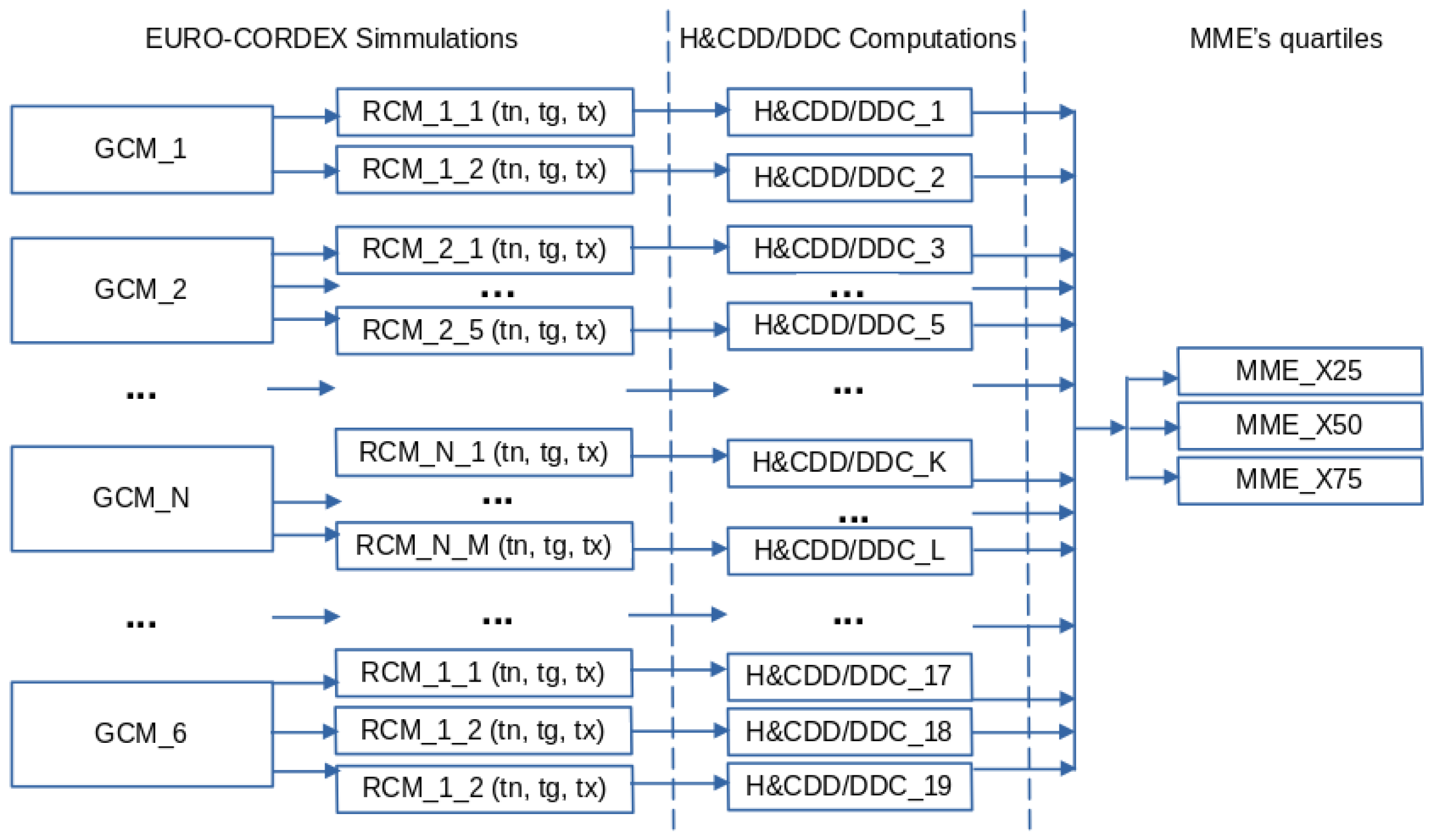
First, the ERA5-Land data for tn, tg, and tx for the reference period, as well as the corresponding data from EURO-CORDEX for the reference and future periods for all 19 combinations of GCMs/RCMs, according to Table 1, are downloaded from the CDS. Next, the EURO-CORDEX data is re-projected from the native rotated grid to the regular ERA5-Land grid using bilinear interpolation, and a spatial subset is selected over the considered domain. Comparing four methods of interpolation, [14] finds that the bilinear method is the most suitable when comparing the root mean square error (RMSE) of temperature between the original data and the interpolated data. Subsequently, we calculate the degree-days and degree-day categories from the ERA5-Land data and the EURO-CORDEX for each model combination, period, and RCP scenario separately, day by day, and lastly summing them for each month. The DDC is expressed as the relative share of the UCD, MCD, MWD, and UWD (See Table 2 again) in the corresponding month. Calculations are performed for both base temperatures. To distinguish the derived parameters, the prefix ’H’ is added for the heating group (i.e., HUCD, HMCD, HMWD, and HUWD as well as CCDD) and ’C’ for the cooling group (i.e., CUCD, CMCD, CMWD, and CUWD as well as HHDD). Finally, we compute the MME’s lower and upper quartile as well as the median and calculate their multiyear monthly means for both periods. The degree-days and the DDC are calculated by specially designed programs written in Fortran using the gfortran compiler part of GNU Compiler Collection (GCC) version 11.2.0; all netCDF file manipulations are performed with the powerful tool Climate Data Operators [45], included in the authors’ purpose-built Linux bash shell scripts. Figure 2 provides an overview of the flowchart summarizing the main data processing parts.

4. Results and Discussion

4.1. Evaluation of Historical Experiments

A crucial first step in determining the accuracy of model data for describing the current degree-day climate and estimating the characteristics of the climate change signal across a region is the quality evaluation of RCM historical simulations [13,34,35].
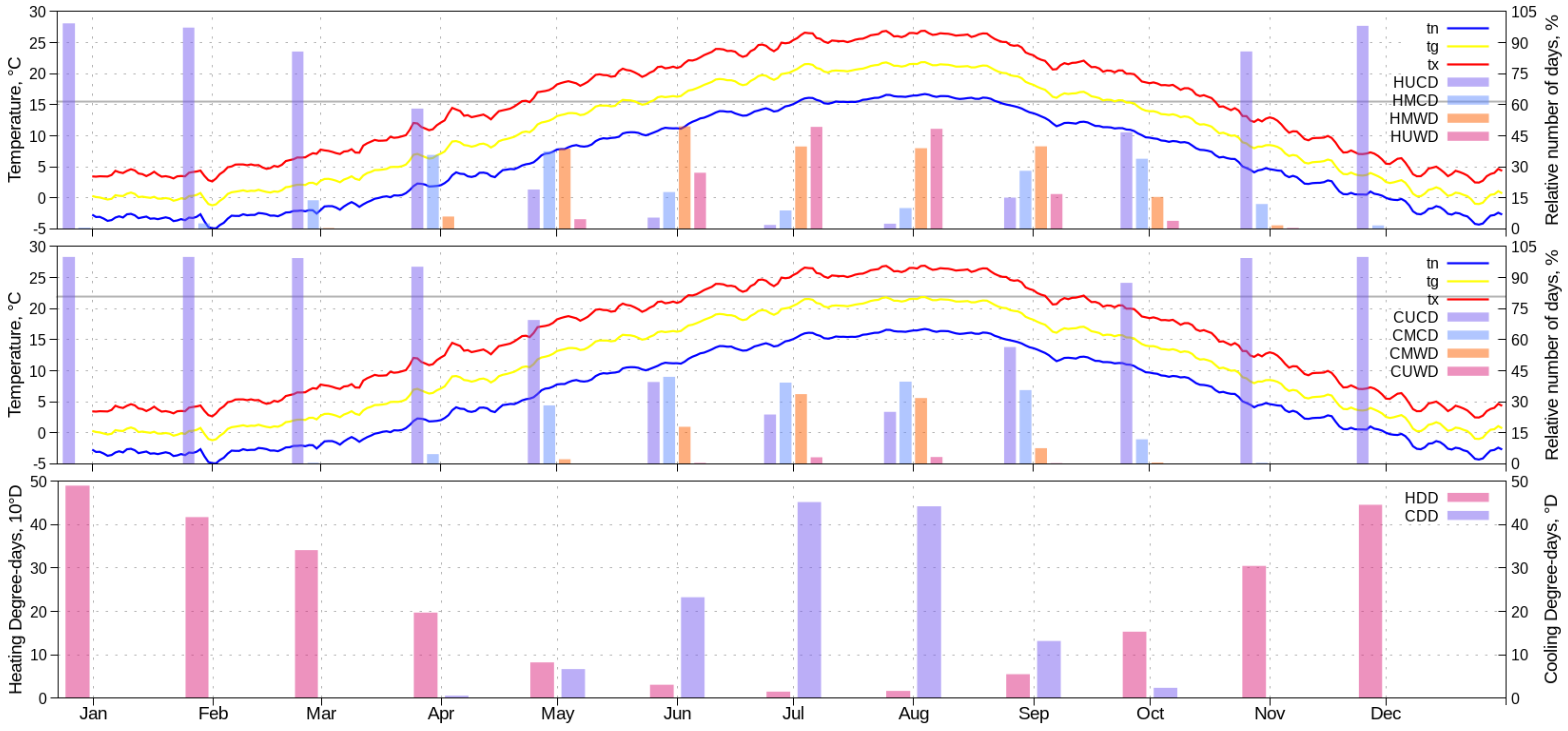
Figure 3 provides an overview of the 30-year monthly means of the area-averaged values (i.e., field means over the domain) of the DDC, HDD, and CDD as well as the 30-year daily means of the tn, tg, and tx over the historical period derived from the the ERA5-Land data.
Generally, all parameters exhibit a clear seasonal cycle. Following the intra-annual changes in the underlying tn, tg, and tx, the DDC, HDD, and CDD exhibit the typical variations characteristic of mid-latitudes. More than 85% of all days in the period November-March are uniformly cold; this fact is clearly expressed according to the cooling criteria due to the higher base temperature. Conversely, the relative share of the heating uniformly warm days is significant only for the summer months and September. The percentage of the cooling uniformly warm days is tiny during the whole year. The fact that the maximum values of the minimum temperature are 4–5 °C lower than the base temperature is indicative in this regard. Even the daily mean temperature remains below this threshold for most of the year. Furthermore, the relative share of the CMCD is always higher than that of the CMWD, including the warm season from April to October. As expected, the combined percentage of the intermittent categories, mostly cold or warm days, is highest in the transitional seasons, more specifically in May and September. This is valid, however, for the heating group only. The interpretation of seasonal variations in heating and cooling degree-days is more straightforward. The maximum of the HDD occurs in January, and the maximum of the CDD occurs in July. It is worth mentioning, however, that the HDD are not zero, even during the summer. This could be attributed to the relatively big geographical share of the mountainous (and relatively cold) areas in the domain. Conversely, due to the significantly higher base temperature, the CDD are practically meaningful only in the summer.
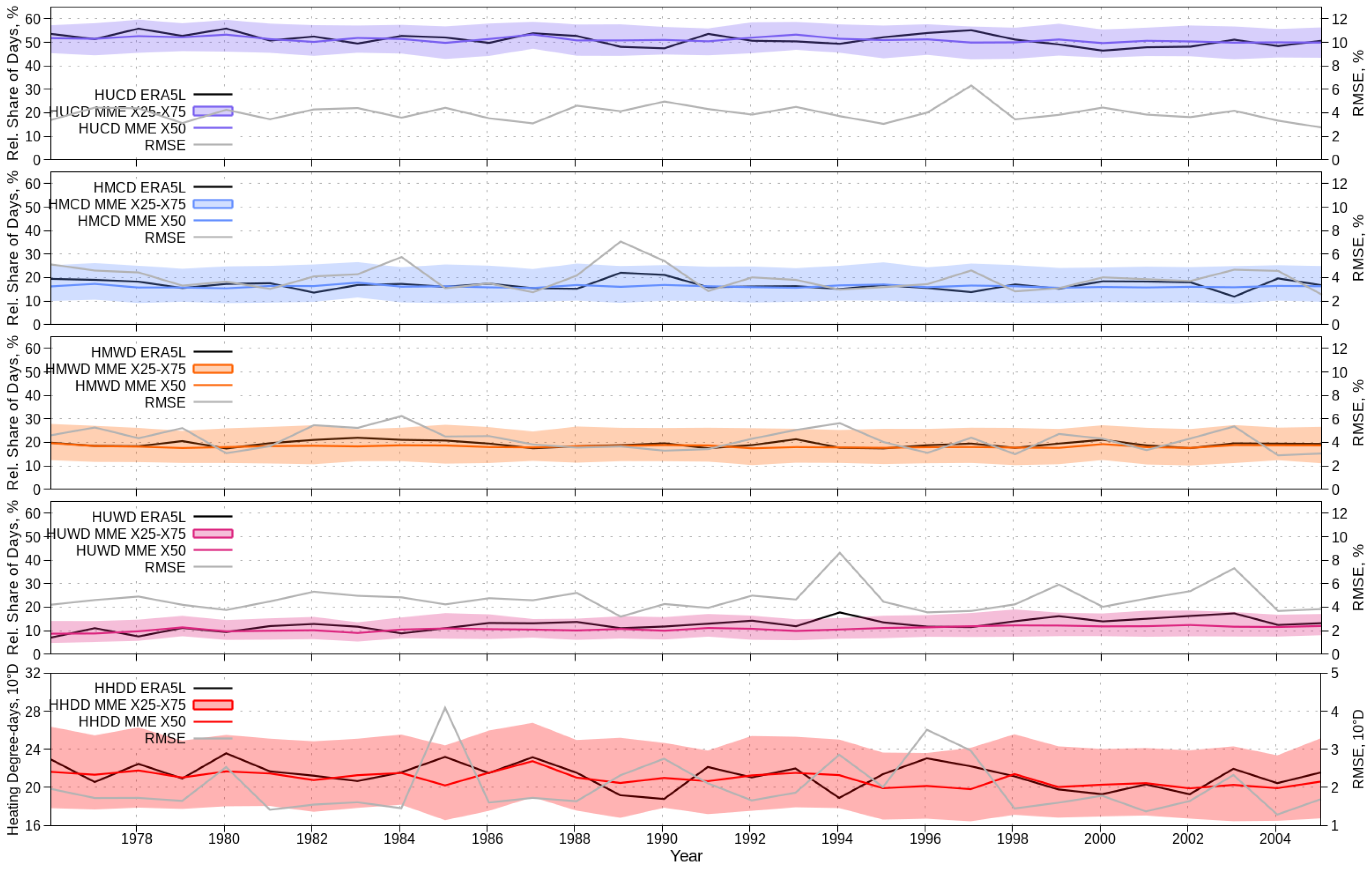
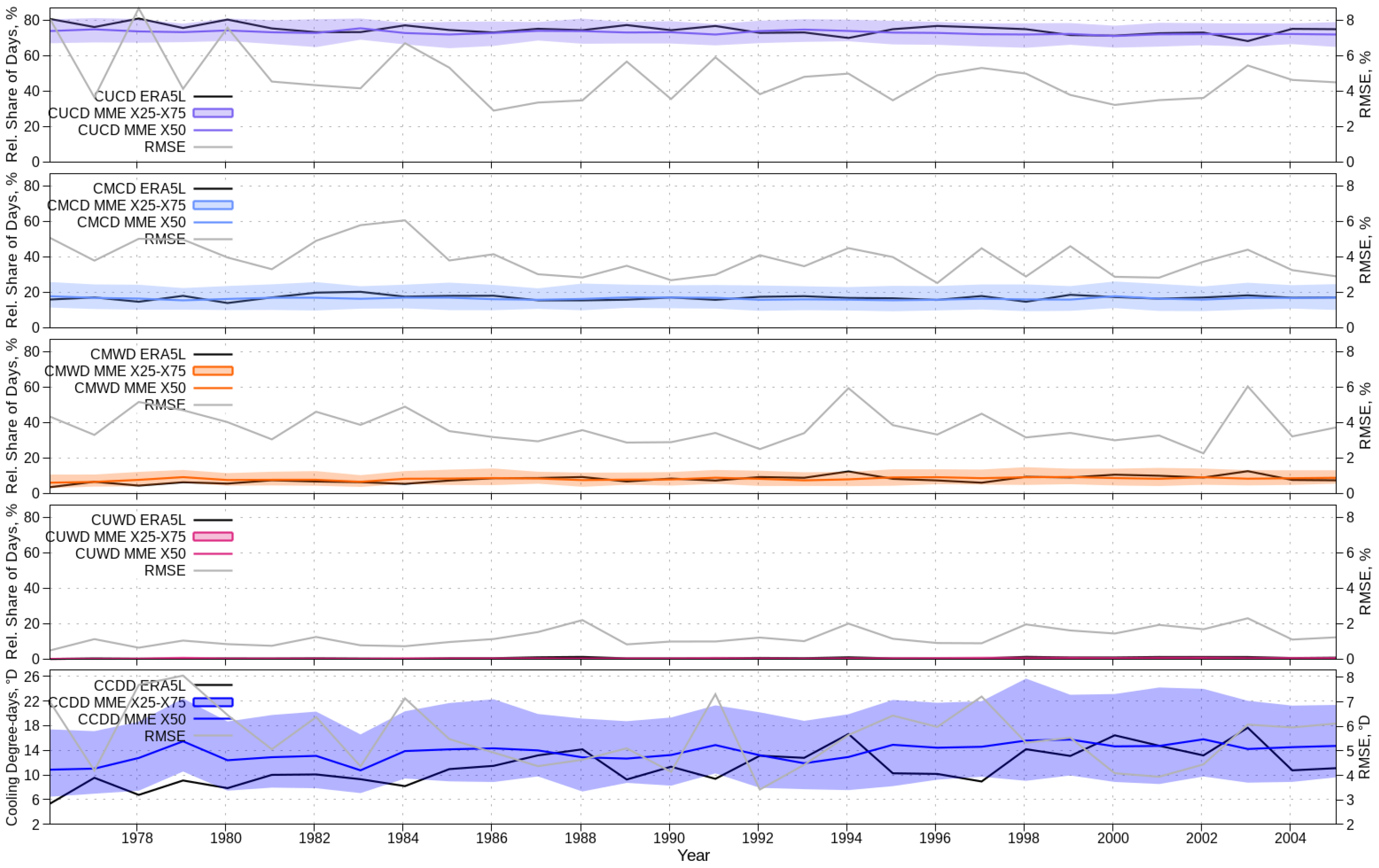
The ability of the RCM MME to reproduce the spatial and temporal variability of the considered parameters for the near past period has been evaluated at annual and multiyear time scales as in [30]. In order to perform the evaluation, the MME output parameters (referred to as the ’model’) are compared with their equivalents calculated using ERA5-Land data (referred to as the ’reference’) in two ways: (i) the MME skill to simulate the long-term evolution of the field mean values of the annual means of the DDC, HDD, and CDD is examined, and (ii) the spatial distribution of the multiyear monthly mean values of the MME X50 is compared with the reference. The performance of the MME X50 is quantified with the RMSE, computed with the reference and the MMEX50, on an annual basis, and in the grid space. The long-term evolution of the considered parameters for the model and the reference is shown in Figure 4 and Figure 5 for the heating and cooling groups, respectively.
The overall first impression from Figure 4 and Figure 5 is that the model reasonably reproduces the long-term variation of the considered parameters of both groups. Most importantly, the reference values of all parameters are in the corresponding MME interquartile ranges X25–X75 during the whole period except a few years, for example, 1985, 1994, and 1996. Subsequently, the RMSE exhibits a maximum in these years. Although MME medians cannot always capture the year-to-year changes of the reference, they are generally relatively close. It is also worth mentioning that the model does not demonstrate any apparent systematic under- or overestimation of the reference in terms of field means.
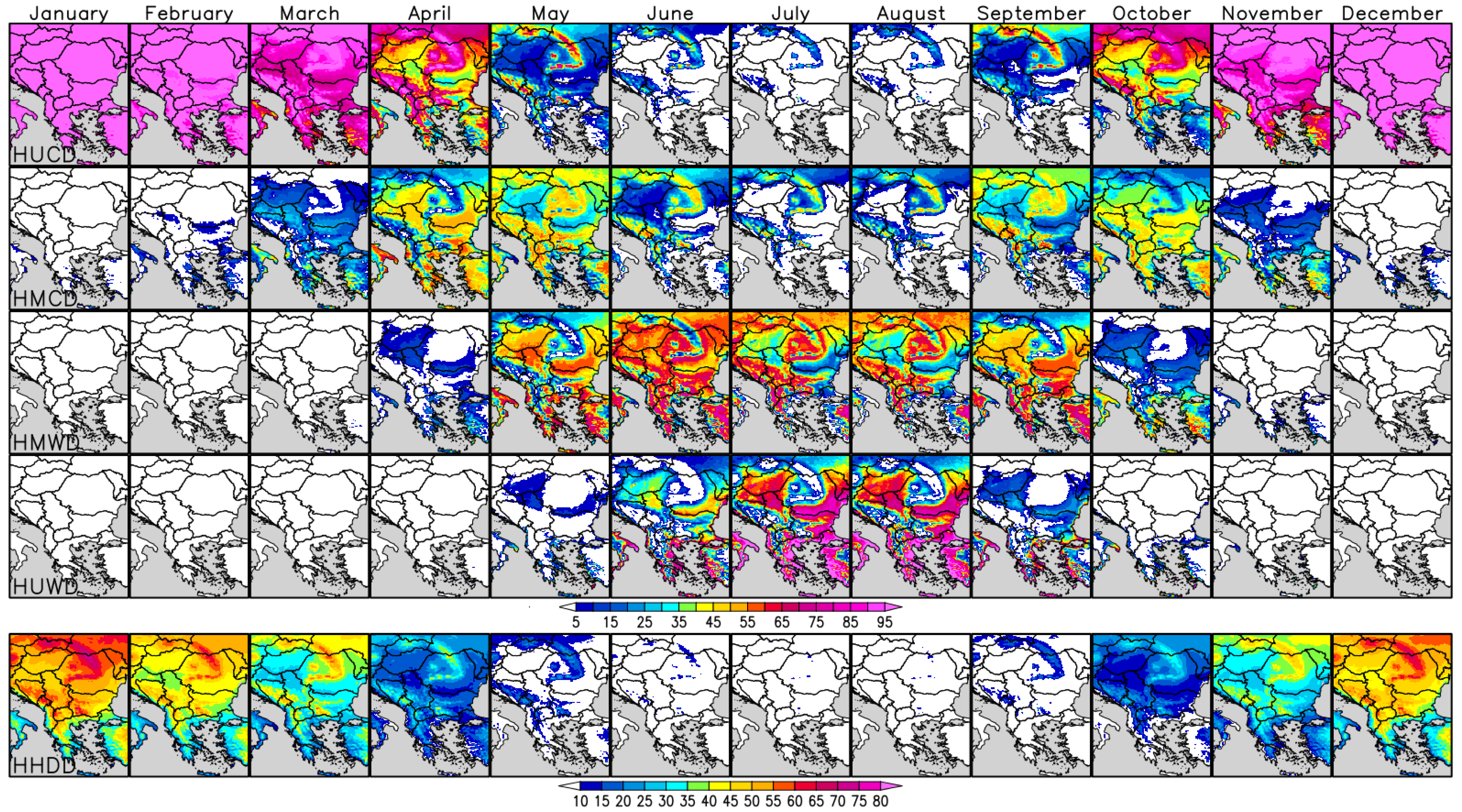
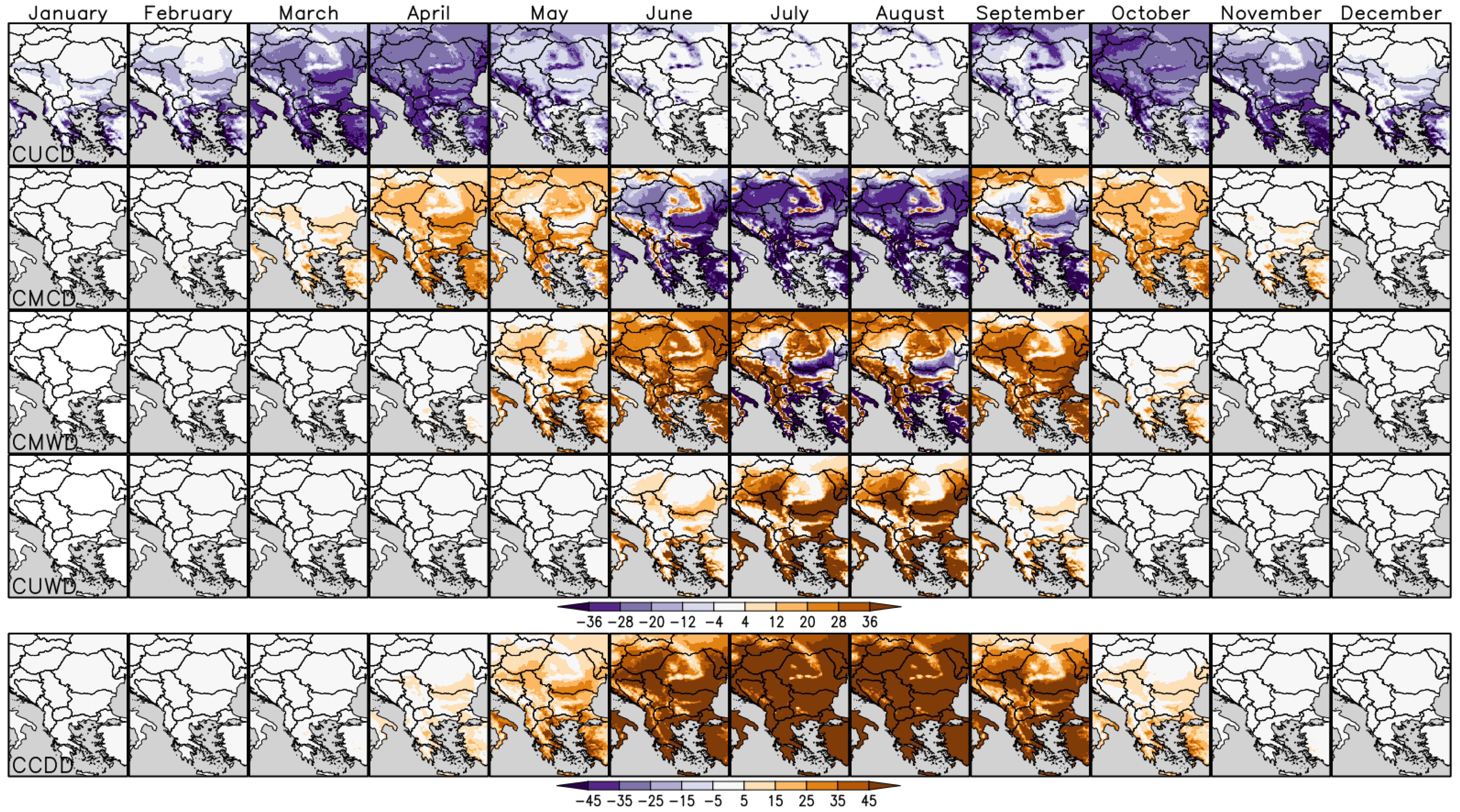
Figure 6 and Figure 7 show an overview of the spatial distribution of the 30-year monthly mean of the considered parameters of the reference.
Figure 6 and Figure 7 reveal, as a whole, a complex picture of variations both in space and time, as well as across the considered parameters. The spatial patterns of the heating and cooling DDCs, as well as HDD and CDD, generally follow the distributions of the underlying tn, tg, and tx in the domain, as we have already shown in our earlier studies [30,33,34]. The south-north gradient and the elevation effects, especially over the main Carpathian ridge (MCR), are well expressed. Most notable are the intra-annual variations of all parameters, which are due to the explicit consideration of the monthly scale of the analysis. Consistent with Figure 3, HUCD from November to March and CUCD from October to April, due to the higher base temperature, are over 85% practically over the whole domain. Conversely, the HUWD is significant only in the summer; the CUWD remains close to zero throughout the year, as already shown in Figure 5. The interim category HMCD exhibits the highest values, between 30% and 50%, over the majority of the domain, in the transitional months of April-May and September-October. The other interim category, HMWD, is predominantly above 30% in May-September, with a maximum in June. Regarding the cooling group, more than one-third of the days from May to September are CMCD. Even in the summer, the relative share of the CMWD is below 30% for most of the domain. It is also worth mentioning that the spatial distribution of HMWD/HUWD, on the one hand, and the CMWD, on the other, demonstrates the highest contrasts in the vertical direction. This is a direct consequence of the fact that the temperature difference during the summer between the overheated plains and relatively cold mountain tops demonstrates seasonal maximum. As expected, the HHDD have a maximum during the winter, reaching in January 400–500 °D over the plains and up to 700 °D over the mountains, mainly the MCR. In the first spring month and the last autumn one, these values are typically 300–400 °D and up to 500 °D. In April and November, HHDD are mostly below 300 °D, and in the rest of the year, from May to September, the HHDD are above 100 °D only in the mountains. Conversely, the cooling degree-days have a maximum in the summer, where their spatial distribution and values in July and August are practically identical. The most prominent hot spots are the lower reaches of the Danube River, part of the Thracian valley (the three-border area between Bulgaria, Greece, and Türkiye), part of the coastal regions of Greece and Türkiye, where CCDD have monthly values of about 75–90 °D in July and August.
We quantify the degree of similarity between the spatial distribution of the multiyear monthly mean values of the MME X50 on the one hand and the reference on the other by the commonly used measure absolute bias (AB) for the DDCs and relative bias (RB) for the heating and cooling degree-days. The selection of AB for the DDCs is reasonable, as they are already expressed as a relative share of days with specific thermal conditions. However, for degree days, the normalization with respect to the reference is relevant; hence, HHDD and CCDD have magnitude differences that are typically up to an order, as previously emphasized in [30].
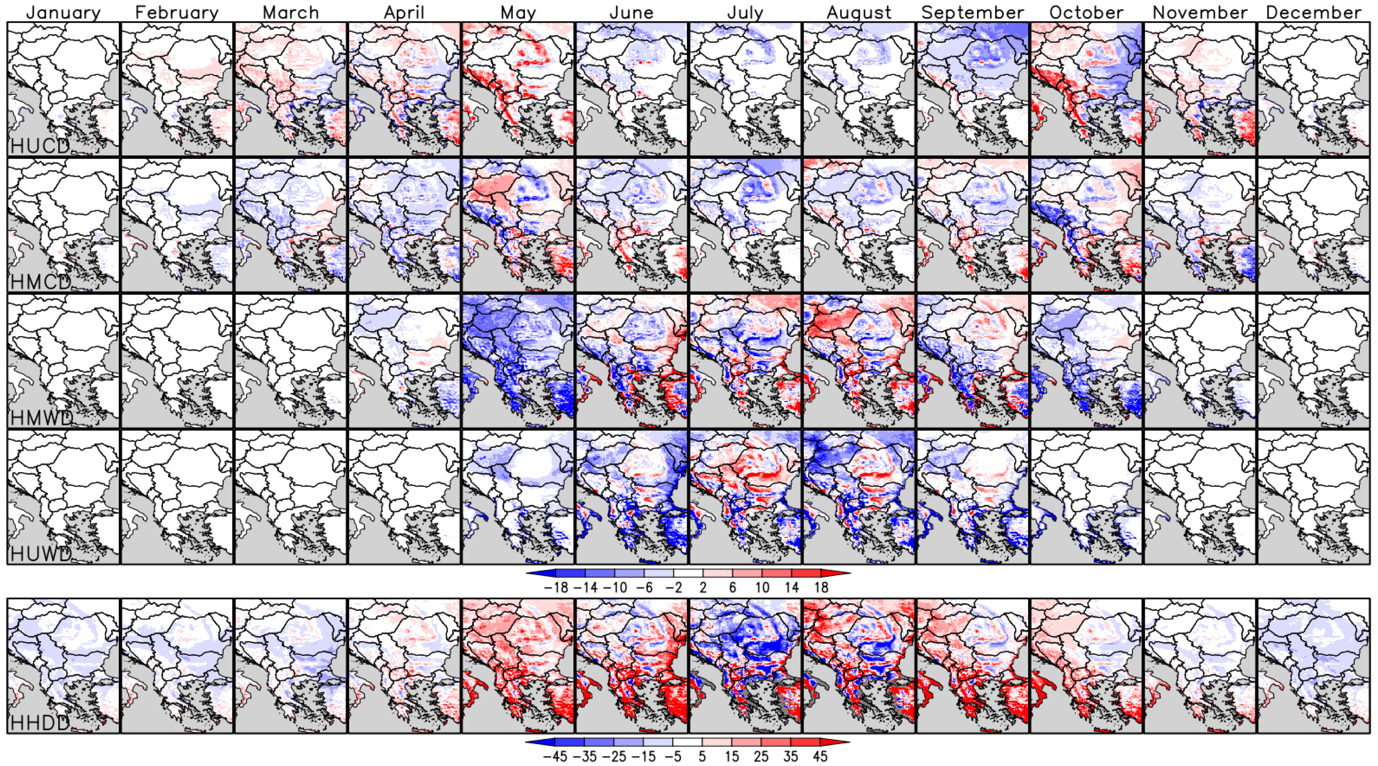
Maps of the MME medians of the parameters considered are not presented for the sake of brevity. Figure 8 and Figure 9 show the spatial distribution of the biases of the parameters from the heating and cooling groups, respectively.
Figure 8 reveals, first of all, that the biases of the heating group parameters are relatively small in the cold period of the year, from November to April. The AB of the DDCs and the RB of the HHDD during this period are typically between −5% and 5%. The absolute values of the biases are significant only for the rest of the year, but the impact of this bias from a practical and economic point of view is minimal, as this period is without heating demand. According to Figure 6, the cooling is reasonable over significant part of the domain for the months May-September only. Figure 9 reveals a significant overestimation of more than 20% of the CCDD in July-September, which is consistent with the underestimation of the CUCD in the same part of the year. This period is characterized by well-expressed cooling and ventilation demand in most of the domain.
A possible explanation of the distinct seasonal variation of the biases of the parameters considered and especially the non-negligible value of these of CCDD and CUCD in the summer is the typical seasonal course of the tn, tg, and tx and their changing proximity to the tb depending on the month as shown in Figure 3. When the daily mean and extreme temperatures are significantly below the base temperature, as in the cold part of the year, small model or MME biases in simulating daily temperatures cannot lead to an erroneous determination of the degree-day category and the degree-days. Conversely, when tn, tg, or tx are close to tb on a particular day, even minor model deviations could cause the allocation of this day in the wrong category and, respectively, the wrong estimation of the degree-days. The last case is typical for the period May-October for the heating group and June-September for the cooling group due to the higher tb. In the latter period, the MME overestimates the daily temperatures, which could explain the distinct warm biases in the fields of the CUCD and CCDD.

4.2. Projections of Future Changes

We calculate the projected changes under the ’realistic’ scenario RCP4.5 and the ’pessimistic’ scenario RCP8.5 for the future period 2066–2095, taking the historical period 1976–2005 as a reference. Changes are expressed in terms of absolute differences, which is the most widely used approach [4,13,19,27] and, additionally, minimizes MME biases [35,46].
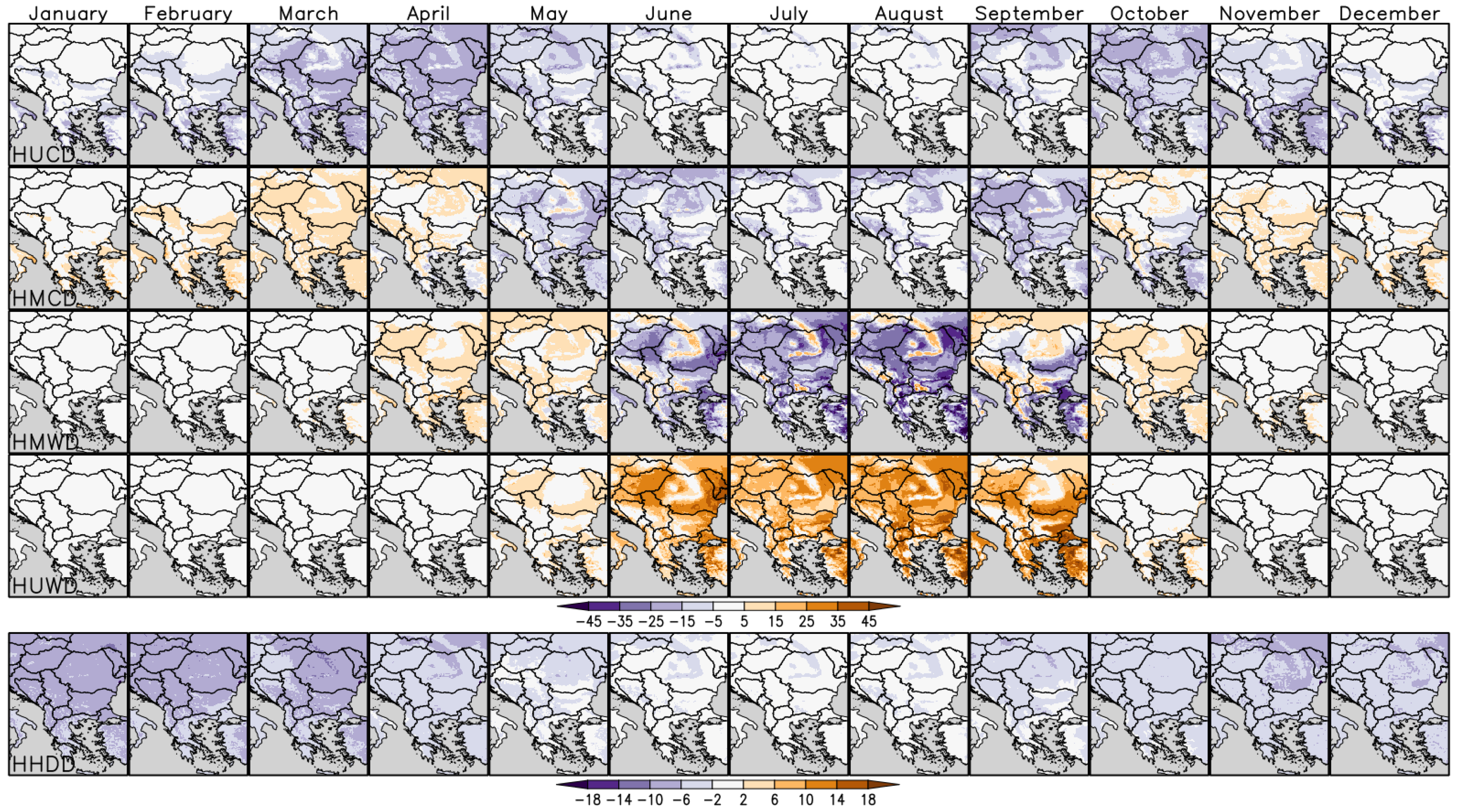
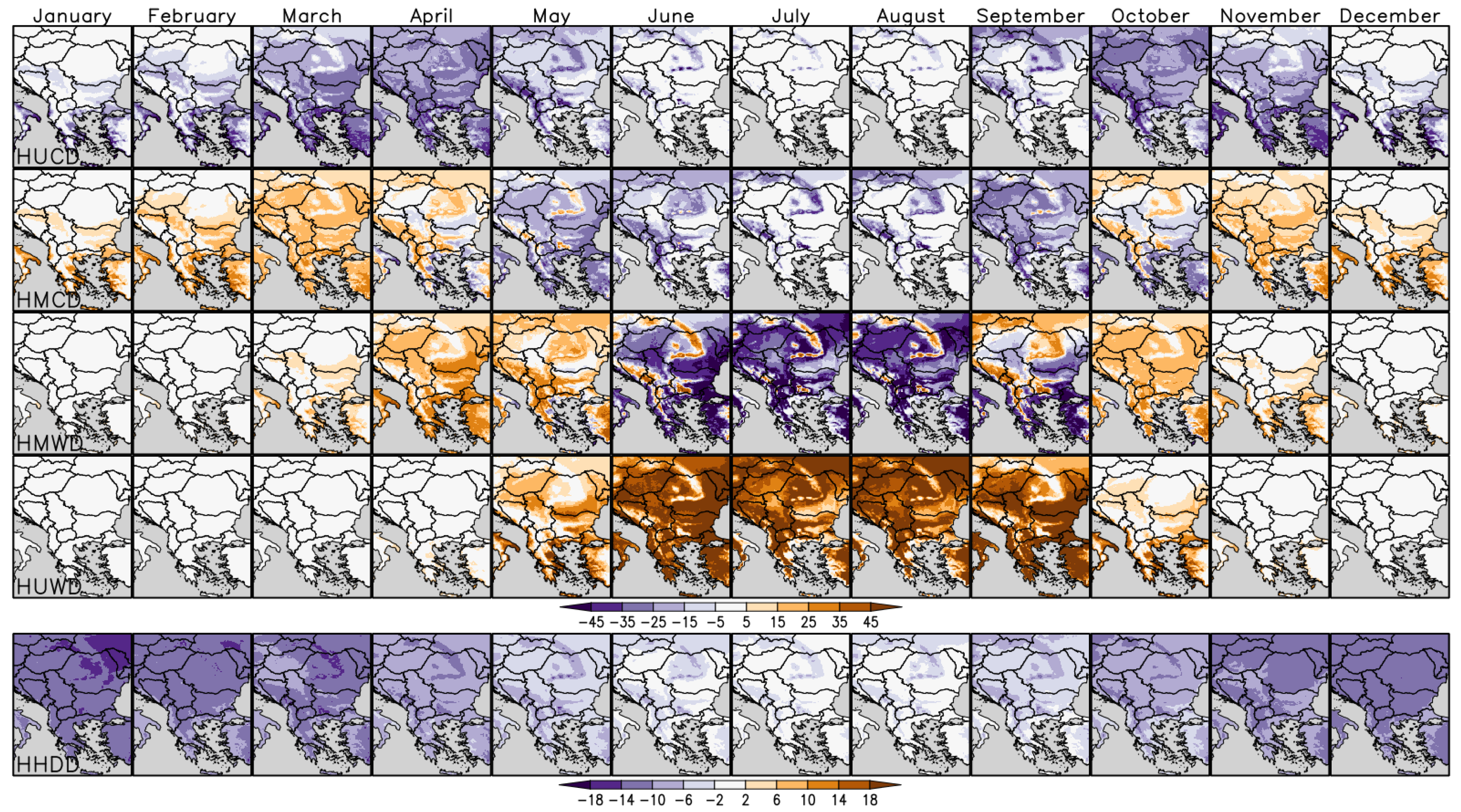
Figure 10 and Figure 11 illustrate the projected absolute change of the multiyear monthly means of the MME X50 of the considered heating group parameters under the RCP4.5 and RCP8.5 scenarios.
Overall, and consistently with the general long-term warming tendency, considering the DDCs, the results indicate a transition toward warmer categories. These changes, however, exhibit essential heterogeneity, both in magnitude and sign, across the domain and throughout the year. The HUCD decreased throughout the year, more significantly in spring (MAM) and autumn (SON), especially in April and October. The transitional categories HMCD and HMWD demonstrate opposite tendencies depending on the month; in March-April and October-November, the increase prevails at the expense of the reduction of the neighboring colder category, HUCD or HMCD, respectively. In contrast, we observe a distinct decrease in HMCD and HMWD in the summer (JJA). An exception is the increase in the HMWD over the mountains, resulting from the decline in the HMCD. Most complex is the spatial distribution of the changes in HMCD in April and October, as well as that of HMWD in September, when negative and positive changes coexist. The change in HUWD is positive for the warm period of the year, with the most significant magnitude in summer. Conversely, the change in HHDD is negative throughout the year, demonstrating a distinct seasonal variation; the magnitude of the reduction is most significant in winter. The primary difference between the two scenarios lies in the degree of expected changes, with a general similarity in the spatial patterns. As expected, the anticipated changes are substantially larger, in absolute terms, under the scenario with the stronger radiative forcing, RCP8.5. Thus, for example, the area-averaged increase in the HUWD under RCP4.5 in JJA ranges from 20% to 30%, and under RCP8.5, it exceeds 35%; the reduction in the HHDD under RCP4.5 remains below 100 °D in DJF, and under RCP8.5, it typically ranges from 100 to 140 °D in the same period.
Figure 12 and Figure 13 shows the projected absolute change of the multiyear monthly means of the MME X50 of the considered cooling group parameters under the RCP4.5 and RCP8.5 scenarios.
Although there are several similarities in the spatial distribution of the cooling DDCs compared to their heating group counterparts, essential differences can also be outlined. These differences are most significant in absolute terms for the transitional categories CMCD and CMWD in the summer. The CMCD is significantly reduced over the plains, whereas it is increased most notably over the mountains, particularly over the MCR. The reduction is due to the shift of days to the neighboring warmer category, CMWD. Subsequently, The CMCD-increase is at the expense of the decrease in CUCD. The largest and spatially most dominant changes in CMWD occur in June and September. Notably, we observe the coexistence of significant changes with opposite signs in the summer months of July and August for this category. Although the increase spatially prevails over certain regions, mainly the listed in Section 4.1 hot spots, we observe a decrease at the expense of the increase of CUWD. We also detect discernible differences for some transitional months. For example, the positive change in CMCD in May appears to be in contrast with the HMCD reduction in the same month. As expected, we detect a significant rise in the CCDD from May to September; in July and August, it typically ranges from 30 to 40 °D under RCP4.5 and from 40 to 50 °D under RCP8.5. Most importantly, the anticipated relative increase in CCDD in the summer months is substantially greater than the relative decrease in HHDD in the winter. This result confirm the key message of the study [18] which is also based on the EURO-CORDEX simulations. It should be noted that the magnitude of the expected rise in September is greater than that of May. This result could be attributed to the already evidenced in [2,3] seasonal shift in the regional warming context and is also consistent with the finding in [34,35] that September tends to behave as a summer month in the projected future climate. As in the case of the HHDD, the results for the CCDD are consistent with the outcomes of [8,13,18] and these of [14,30] based on CMIP6 simulations.
Finally, we will discuss the absolute changes of the 30-year monthly means of the area-averaged values under the RCP4.5 and RCP8.5 of the future period, with respect to the reference for the parameters of the heating and cooling group shown in Figure 14 and Figure 15 respectively. Similarly to the discussed in Section 4.1 area-averaged values, these quantities are calculated with the cdo operator ’fieldmean’.
These box-plots outline more clearly than the maps in Figure 12 and Figure 13 the differences in the projected changes depending on the scenario—for all parameters in both groups, the absolute value for RCP8.5 is essentially larger than that for RCP4.5. The reduction of the HUCD is strongest in spring and autumn, reaching a maximum in April with values of approximately 15% (i.e., 4–5 days) for RCP4.5 and 25% (7–8 days) for RCP8.5. Generally, the HMCD exhibits an increase during the cold period of the year (November to April) and a decrease for the rest of the year. The other intermittent category, HMWD, exhibits an increase in the spring, with a maximum in April and again in October and November. According to the magnitude, the most prominent are the positive changes of the HMWD, especially in the summer months. The increase in June and August is almost the same reaching about 20% (5–6 days) for RCP4.5 and 30% (18 days) for RCP8.5. This remarkable rise comes at the expense of a reduction in all other DDCs, especially the HMWD. It is worth mentioning that the overall pattern of the expected changes for September is similar to that of the summer months.
As expected, the change in HHDD is negative for the whole year. The seasonal variation is apparent, the magnitude of the reduction is most significant in winter, reaching a maximum of 70 °D for RCP4.5 and 120–125 °D for RCP8.5.
As emphasized in Section 4.1, the parameters of the cooling group are meaningful for the warm period of the year. The most significant from the end-user view is the increase in CUWD in July and August of about 28–29% (9 days). Unlike the heating group, this increase is accompanied by a rise in CMWD. The difference between June and July-August is also noticeable. The increase of the CCDD in these two months is 35–40 °D for the realistic, and almost 90 °D for the pessimistic scenario. The increase of the CCDD in September is essentially larger than that of May for both scenarios. It is worth mentioning the non-negligible rise in cooling demand, even in the middle of spring (April) and autumn (October).

5. Conclusions and Outlook

The paper presents a comprehensive study of the heating and cooling degree-days and the degree-days categories for the near past, and the AR5 RCP4.5 and RCP8.5 scenario-driven future over Southeast Europe based on an elaborated methodology and performed using a large number of combinations of driving GCMs and RCMs from EURO-CORDEX with horizontal resolution at 0.11°. Hence, the study is performed on a monthly scale, allowing the assessment of the intra-annual variations, and due to the explicit consideration of the degree-day categories, the study is novel, according to our knowledge.
The peculiar effects of global warming are especially recognizable over the considered domain of SEEu as part of the broader Mediterranean area. The Mediterranean Sea and the Black Sea are almost closed water basins; they are relatively shallow and, according to [5], their waters warm ten times faster than those of the oceans, causing a more rapid temperature increase of the region compared to the global scale.
In general, the presented results for the heating and cooling degree days demonstrate a high level of consistency with our previous studies [33,34,35], investigations of other authors utilizing the same computational framework (UKMO methodology, CMIP5 simulations, and RCP scenarios) [8,13,18,19,23], and recent commensurable CMIP6-based works [14,30]. In agreement with the majority of recent research in the field, we show a steady growth in cooling and a decrease in heating demand, which leads to a decrease in HDD that is smaller than the increase in CDD in relative terms and, additionally, a shift toward warmer degree-day categories. Furthermore, and due to consideration of the monthly, rather than annual, time scale, our results for the projected future climate show that cooling demand begins earlier in late spring and continues into early autumn, resulting in a longer cooling season and a shorter heating season. This fact, alongside the general increase of the CCDD, will result in long-term changes in the seasonal patterns of energy consumption, with the cooling season increasingly overlapping with the heating season of the past. Regardless of the fact that the overall energy demand is expected to decrease due to lower heating needs, cooling will become a growing challenge in SEEu. Although there are some relatively simple semi-empirical approaches [47], the relationship between climate and thermal energy demand is complex, nonlinear, and not free from uncertainties. However, knowledge of the anticipated change of the mean thermal conditions on the one hand and the extreme events (hot or cold spells, responsible for a peak power load) on the other gives a starting point for dimensioning HVAC systems [32]. As a whole, the magnitude of the revealed long-term changes is generally proportional to the radiative forcing, i.e., stronger for the ’pessimistic’ scenario RCP8.5 than the ’realistic’ scenario RCP4.5. These outcomes are consistent with the well-documented general temperature trend over the region. They are a direct result of the steady increase in temperature in the gradually warming climate of the region. However, the projected changes exhibit essential spatial heterogeneity, both in magnitude and sign, which is especially notable because of the fine grid spacing utilized. The fine grid spacing allows, in particular, the designation of coexisting opposite tendencies for some degree-day categories in the transitional months over the mountains on the one hand and over the plains on the other. The month-to-month variations are also significant, emphasizing the importance of considering sub-annual temporal scales in further degree-days research.
The current evaluation has limitations in common with other research projects that use comparable methodology and data sources, such as [19,41]. First, we have not performed bias-correction (BC) of the input EURO-CORDEX data, which, according to [4,13], could affect the accuracy of the results. More specifically, the pointed in Section 4.1 disagreement of the MME values with respect to the reference, especially in the transitional months when small temperature deviations are important for the degree-days classification, could be attributed to the absence of bias correction. However, it should be emphasized that BC is objectively hampered by the lack of a reliable enough region-wide observation-based data set. Hence, E-OBS of ECA &D exhibits some non-negligible issues over part of the domain [30]. Furthermore, our investigation in [46] dedicated on key climate indices similar to the degree-days, demonstrates that the difference between the future and the past, which is the core of the present article, minimizes the systematic biases of GCM/RCM. The population dynamics are also not included in the degree-days assessment framework. Although methodologically important [30], its exclusion from the analysis is determined by the absence of reliable demographic data over SEEu, which is compatible with the RCP scenarios [13]. More specifically, the Eurostat Geostat dataset [48] that is used as data source in the similar studies [8,13] does not contain data for countries that are not member states of the EU but occupies a significant part of the considered domain.
The study could be continued in many ways, and the natural next step is using input data from the next phase of EURO-CORDEX based on the CMIP6 GCM simulations. Future research should elucidate the nexus between regional warming and the urban heat island (UHI) effect, as numerous cities within the region are affected by this phenomenon [2,3,5,18]. According to the study [49] for the Greek cities of Patra and Calamata, the UHI substantially modifies the HVAC requirements compared with the rural surroundings. Due to the implemented computation methodology, which premises the comparison of all three daily temperatures, tn, tg, and tx, with prescribed threshold (tb), the HDD and CDD could be treated in a broader context (i.e., beyond the HVAC implementation) as compound climate indices. As stated in [18], they can also be considered as a proxy of the deviations from the optimum conditions for outdoor activities such as agriculture and tourism.
Most significantly, the current study unequivocally affirms the importance of the anticipated long-term changes of all analyzed parameters over the considered region in the projected RCP scenario-driven future toward the end of the 21st century. Their subsequent effect is a substantial alteration in the demand for heating, cooling, and ventilation, which, in turn, affects the capacity and seasonality of energy production and transportation. Despite the limitations covered in this section, stakeholders and policymakers could use the current results—which are far more detailed than those from studies conducted with coarser resolution, on an annual scale, and without consideration of the degree-day categories—as a scientific basis for putting optimization and mitigation strategies into practice.

Author Contributions

Conceptualization, H.C.; methodology, H.C.; software, H.C. and K.S.; validation, K.S.; formal analysis, K.S.; investigation, H.C.; resources, K.S. and H.C.; data curation, K.S.; writing—original draft preparation, H.C.; writing—review and editing, H.C. and K.S.; visualization, H.C. All authors have read and agreed to the published version of the manuscript.

Funding

This research received no external funding.

Institutional Review Board Statement

Not applicable.

Informed Consent Statement

Not applicable.

Data Availability Statement

The raw input data are downloaded from the Climate Data Store of the Copernicus Climate Change Service https://doi.org/10.24381/cds.bc91edc3, (accessed on 12 February 2024). The datasets, containing all considered degree-days parameters, are available on reasonable request to the corresponding author.

Acknowledgments

We express our deep gratitude to all institutions (primary GCM and RCM vendors, ECMWF, C3S-CDS, MPI-M) that provide free-of-charge data and software. Not least, we thank the four anonymous reviewers for their comments and suggestions which led to an overall improvement of the original manuscript.

Conflicts of Interest

The authors declare no conflicts of interest.

Abbreviations

The following abbreviations are used in this manuscript:
ABAbsolute Bias
AR5Fifth Assessment Report (of the IPCC)
C3SCopernicus Climate Change Service
CCDDCooling Degree-day
CDSClimate Data Store (of the Copernicus Climate Change Service)
CMIP5Coupled Model Intercomparison Project Phase 5
DDCDegrree-day Category
ECMWFEuropean Centre for Medium-Range Weather Forecasts
GCMGlobal Circulation Model
HHDDHeating Degree-day
HVACHeating, Ventilating, and Air-conditioning
IPCCIntergovernmental Panel on Climate Change
MCDMostly Cold Day
MMEMultimodel ensemble
MWDMostly Warm Day
RCMRegional Climate Model
RCPRepresentative Concentration Pathway
SEEuSoutheast Europe
UCDUniformly Cold Day
UKMOUnited Kingdom Meteorological Office
UWDUniformly Warm Day

References

  1. IPCC. Summary for Policymakers. In Climate Change 2023: Synthesis Report. Contribution of Working Groups I, II and III to the Sixth Assessment Report of the Intergovernmental Panel on Climate Change; IPCC: Geneva, Switzerland, 2023; pp. 1–34. [Google Scholar] [CrossRef]
  2. Lionello, P.; Abrantes, F.; Congedi, L.; Dulac, F.; Gacic, M.; Gomis, D.; Goodess, C.; Hoff, H.; Kutiel, H.; Luterbacher, J.; et al. Introduction: Mediterranean Climate—Background Information. In The Climate of the Mediterranean Region; Elsevier Inc.: Amsterdam, The Netherlands, 2012; pp. 35–90. [Google Scholar] [CrossRef]
  3. Xoplaki, E.; Trigo, R.M.; García-Herrera, R.; Barriopedro, D.; D’Andrea, F.; Fischer, E.M.; Gimeno, L.; Gouveia, C.; Hernández, E.; Kuglitsch, F.G.; et al. Large-Scale Atmospheric Circulation Driving Extreme Climate Events in the Mediterranean and Its Related Impacts. In The Climate of the Mediterranean Region; Elsevier Inc.: Amsterdam, The Netherlands, 2012; pp. 347–417. [Google Scholar] [CrossRef]
  4. Andrade, C.; Mourato, S.; Ramos, J. Heating and Cooling Degree-Days Climate Change Projections for Portugal. Atmosphere 2021, 12, 715. [Google Scholar] [CrossRef]
  5. Salata, F.; Falasca, S.; Ciancio, V.; Curci, G.; de Wilde, P. Climate-Change Related Evolution of Future Building Cooling Energy Demand in a Mediterranean Country. Energy Build. 2023, 290, 113112. [Google Scholar] [CrossRef]
  6. Pangsy-Kania, S.; Biegańska, J.; Flouros, F.; Sokół, A. Heating and Cooling Degree-Days vs Climate Change in Years 1979–2021. Evidence from the European Union and Norway. Econ. Environ. 2024, 88, 619. [Google Scholar] [CrossRef]
  7. Mehregan, M.; Naminezhad, A.; Vakili, S.; Delpisheh, M. Building Energy Model Validation and Estimation Using Heating and Cooling Degree Days (HDD–CDD) Based on Accurate Base Temperature. Energy Sci. Eng. 2022, 10, 3638–3649. [Google Scholar] [CrossRef]
  8. Larsen, M.A.D.; Petrović, S.; Radoszynski, A.M.; McKenna, R.; Balyk, O. Climate Change Impacts on Trends and Extremes in Future Heating and Cooling Demands over Europe. Energy Build. 2020, 226, 110397. [Google Scholar] [CrossRef]
  9. Petri, Y.; Caldeira, K. Impacts of Global Warming on Residential Heating and Cooling Degree-Days in the United States. Sci. Rep. 2015, 5, 12427. [Google Scholar] [CrossRef]
  10. Buonocore, J.J.; Salimifard, P.; Magavi, Z.; Allen, J.G. Inefficient Building Electrification Will Require Massive Buildout of Renewable Energy and Seasonal Energy Storage. Sci. Rep. 2022, 12, 11931. [Google Scholar] [CrossRef]
  11. Lyu, J.; Ono, T.; Sato, A.; Hagishima, A.; Tanimoto, J. Seasonal Variation of Residential Cooling Use Behaviour Derived from Energy Demand Data and Stochastic Building Energy Simulation. J. Build. Eng. 2022, 49, 104067. [Google Scholar] [CrossRef]
  12. Mastrucci, A.; van Ruijven, B.; Byers, E.; Poblete-Cazenave, M.; Pachauri, S. Global Scenarios of Residential Heating and Cooling Energy Demand and CO2 Emissions. Clim. Change 2021, 168, 14. [Google Scholar] [CrossRef]
  13. Spinoni, J.; Vogt, J.V.; Barbosa, P.; Dosio, A.; McCormick, N.; Bigano, A.; Füssel, H. Changes of Heating and Cooling Degree-days in Europe from 1981 to 2100. Int. J. Climatol. 2017, 38, e191–e208. [Google Scholar] [CrossRef]
  14. Filahi, H.; Omrani, H.; Claudel, S.; Drobinski, P. Temporal Fragmentation of the Energy Demand in Europe: Impact of Climate Change on the Maneuverability of Energy System. Clim. Serv. 2024, 34, 100469. [Google Scholar] [CrossRef]
  15. Pérez-Andreu, V.; Aparicio-Fernández, C.; Martínez-Ibernón, A.; Vivancos, J.-L. Impact of Climate Change on Heating and Cooling Energy Demand in a Residential Building in a Mediterranean Climate. Energy 2018, 165, 63–74. [Google Scholar] [CrossRef]
  16. Skarbit, N.; Unger, J.; Gál, T. Projected Values of Thermal and Precipitation Climate Indices for the Broader Carpathian Region Based on EURO-CORDEX Simulations. Hung. Geogr. Bull. 2022, 71, 325–347. [Google Scholar] [CrossRef]
  17. Badescu, V.; Zamfir, E. Degree-Days, Degree-Hours and Ambient Temperature Bin Data from Monthly-Average Temperatures (Romania). Energy Convers. Manag. 1999, 40, 885–900. [Google Scholar] [CrossRef]
  18. Karagiannids, A.; Lagouvardos, K.; Kotroni, V.; Galanaki, E. Analysis of Current and Future Heating and Cooling Degree Days over Greece Using Observations and Regional Climate Model Simulations. Environ. Sci. Proc. 2023, 26, 149. [Google Scholar] [CrossRef]
  19. Tringa, E.; Tolika, K.; Tsoka, S.; Anagnostopoulou, C.; Kostopoulou, E. Assessing Future Changes in Heating and Cooling Degree Days Using Multiple Base Temperatures for Cultural Heritage Sites in Greece: A Case Study of Thessaloniki and Delphi. Sci. Total Environ. 2025, 977, 179352. [Google Scholar] [CrossRef]
  20. Büyükalaca, O.; Bulut, H.; Yılmaz, T. Analysis of Variable-Base Heating and Cooling Degree-Days for Turkey. Appl. Energy 2001, 69, 269–283. [Google Scholar] [CrossRef]
  21. Yildiz, I.; Sosaoglu, B. Spatial Distributions of Heating, Cooling, and Industrial Degree-Days in Turkey. Theor. Appl. Climatol. 2007, 90, 249–261. [Google Scholar] [CrossRef]
  22. Janković, A.; Podraščanin, Z.; Djurdjevic, V. Future Climate Change Impacts on Residential Heating and Cooling Degree Days in Serbia. IDŐJÁRÁS 2019, 123, 351–370. [Google Scholar] [CrossRef]
  23. Spinoni, J.; Vogt, J.; Barbosa, P. European Degree-day Climatologies and Trends for the Period 1951–2011. Int. J. Climatol. 2014, 35, 25–36. [Google Scholar] [CrossRef]
  24. Ürge-Vorsatz, D.; Khosla, R.; Bernhardt, R.; Chan, Y.C.; Vérez, D.; Hu, S.; Cabeza, L.F. Advances Toward a Net-Zero Global Building Sector. Annu. Rev. Environ. Resour. 2020, 45, 227–269. [Google Scholar] [CrossRef]
  25. Giorgi, F.; Mearns, L.O. Approaches to the Simulation of Regional Climate Change: A Review. Rev. Geophys. 1991, 29, 191–216. [Google Scholar] [CrossRef]
  26. Kotlarski, S.; Keuler, K.; Christensen, O.B.; Colette, A.; Déqué, M.; Gobiet, A.; Goergen, K.; Jacob, D.; Lüthi, D.; van Meijgaard, E.; et al. Regional Climate Modeling on European Scales: A Joint Standard Evaluation of the EURO-CORDEX RCM Ensemble. Geosci. Model Dev. 2014, 7, 1297–1333. [Google Scholar] [CrossRef]
  27. Sillmann, J.; Kharin, V.V.; Zwiers, F.W.; Zhang, X.; Bronaugh, D. Climate Extremes Indices in the CMIP5 Multimodel Ensemble: Part 2. Future Climate Projections. J. Geoph. Res. Atmos. 2013, 118, 2473–2493. [Google Scholar] [CrossRef]
  28. Merrifield, A.L.; Brunner, L.; Lorenz, R.; Medhaug, I.; Knutti, R. An Investigation of Weighting Schemes Suitable for Incorporating Large Ensembles into Multi-Model Ensembles. Earth Sys. Dyn. 2020, 11, 807–834. [Google Scholar] [CrossRef]
  29. Herger, N.; Abramowitz, G.; Knutti, R.; Angélil, O.; Lehmann, K.; Sanderson, B.M. Selecting a Climate Model Subset to Optimise Key Ensemble Properties. Earth Sys. Dyn. 2018, 9, 135–151. [Google Scholar] [CrossRef]
  30. Chervenkov, H.; Slavov, K. Population-Weighted Degree-Days over Southeast Europe—Near Past Climate Evaluation and Future Projections with NEX-GDDP CMIP6 Ensemble. Climate 2025, 13, 66. [Google Scholar] [CrossRef]
  31. Jacob, D.; Kotova, L.; Teichmann, C.; Sobolowski, S.P.; Vautard, R.; Donnelly, C.; Koutroulis, A.G.; Grillakis, M.G.; Tsanis, I.K.; Damm, A.; et al. Climate Impacts in Europe under +1.5 °C Global Warming. Earths Fut. 2018, 6, 264–285. [Google Scholar] [CrossRef]
  32. Berger, M.; Worlitschek, J. The Link between Climate and Thermal Energy Demand on National Level: A Case Study on Switzerland. Energy Build. 2019, 202, 109372. [Google Scholar] [CrossRef]
  33. Chervenkov, H.; Ivanov, V.; Gadzhev, G.; Ganev, K.; Melas, D. Degree-Day Climatology over Central and Southeast Europe for the Period 1961-2018 — Evaluation in High Resolution. Cybern. Inf. Technol. 2020, 20, 166–174. [Google Scholar] [CrossRef]
  34. Ivanov, V.; Chervenkov, H.; Gadzhev, G.; Ganev, K. Degree-days and agro-meteorological Indices in the Projected Future Climate over Southeast Europe. In Proceedings of the SGEM International Multidisciplinary Scientific GeoConference EXPO Proceedings, Albena, Bulgaria, 18–24 August 2020; Surveying Geology & Mining Ecology Management (SGEM): Albena, Bulgaria, 2020. [Google Scholar] [CrossRef]
  35. Chervenkov, H.; Gadzhev, G.; Ivanov, V.; Ganev, K. Degree-Days and Agro-Meteorological Indices in CMIP5 RCP8.5 Future Climate—Results for Central and Southeast Europe. Stud. Syst. Decis. Control 2021, 19–30. [Google Scholar] [CrossRef]
  36. Cramer, W.; Guiot, J.; Fader, M.; Garrabou, J.; Gattuso, J.-P.; Iglesias, A.; Lange, M.A.; Lionello, P.; Llasat, M.C.; Paz, S.; et al. Climate Change and Interconnected Risks to Sustainable Development in the Mediterranean. Nat. Clim. Chang. 2018, 8, 972–980. [Google Scholar] [CrossRef]
  37. Climate Data Store (CDS) of the Copernicus Climate Change Service (C3S). Available online: https://cds.climate.copernicus.eu/datasets/projections-cordex-domains-single-levels?tab=overview (accessed on 12 February 2024).
  38. Muñoz-Sabater, J.; Dutra, E.; Agustí-Panareda, A.; Albergel, C.; Arduini, G.; Balsamo, G.; Boussetta, S.; Choulga, M.; Harrigan, S.; Hersbach, H.; et al. ERA5-Land: A State-of-the-Art Global Reanalysis Dataset for Land Applications. Earth Syst. Sci. Data 2021, 13, 4349–4383. [Google Scholar] [CrossRef]
  39. Guo, C.; Ning, N.; Guo, H.; Tian, Y.; Bao, A.; De Maeyer, P. Does ERA5-Land Effectively Capture Extreme Precipitation in the Yellow River Basin? Atmosphere 2024, 15, 1254. [Google Scholar] [CrossRef]
  40. Jacob, D.; Petersen, J.; Eggert, B.; Alias, A.; Christensen, O.B.; Bouwer, L.M.; Braun, A.; Colette, A.; Déqué, M.; Georgievski, G.; et al. EURO-CORDEX: New High-Resolution Climate Change Projections for European Impact Research. Reg. Environ. Change 2014, 14, 563–578. [Google Scholar] [CrossRef]
  41. Kotova, L.; Leissner, J.; Winkler, M.; Kilian, R.; Bichlmair, S.; Antretter, F.; Moßgraber, J.; Reuter, J.; Hellmund, T.; Matheja, K.; et al. Making Use of Climate Information for Sustainable Preservation of Cultural Heritage: Applications to the KERES Project. Herit. Sci. 2023, 11, 18. [Google Scholar] [CrossRef]
  42. Thomson, A.M.; Calvin, K.V.; Smith, S.J.; Kyle, G.P.; Volke, A.; Patel, P.; Delgado-Arias, S.; Bond-Lamberty, B.; Wise, M.A.; Clarke, L.E.; et al. RCP4.5: A Pathway for Stabilization of Radiative Forcing by 2100. Clim. Change 2011, 109, 77–94. [Google Scholar] [CrossRef]
  43. Riahi, K.; Rao, S.; Krey, V.; Cho, C.; Chirkov, V.; Fischer, G.; Kindermann, G.; Nakicenovic, N.; Rafaj, P. RCP 8.5–A Scenario of Comparatively High Greenhouse Gas Emissions. Clim. Change 2011, 109, 33–57. [Google Scholar] [CrossRef]
  44. CIBSE TM41, 2006 (TM41: Degree Days: Theory & Application, by the Chartered Institution of Building Services Engineers (CIBSE). Available online: http://refhub.elsevier.com/S0048-9697(25)00988-X/rf0230 (accessed on 4 March 2024).
  45. Schulzweida, U. CDO User Guide (Version 2.0.0). 30 October 2020. Available online: https://zenodo.org/record/5614769#.Yk027ihBxPY (accessed on 23 February 2024).
  46. Chervenkov, H.; Spiridonov, V. Bias Correcting of Selected ETCCDI Climate Indices for Projected Future Climate. In Large-Scale Scientific Computing; Springer International Publishing: Cham, Switzerland, 2020; pp. 92–299. ISBN 9783030410315. [Google Scholar]
  47. Frasca, F.; Siani, A.M.; Bertolin, C. Energy Demand for Indoor Climate Control in Museums: Challenges and Perspectives in Time of a Changing Climate. Procedia Struct. Integr. 2024, 55, 32–38. [Google Scholar] [CrossRef]
  48. Eurostat, GEOSTAT—Eurostat, Geostat. 2016. Available online: https://ec.europa.eu/eurostat/web/gisco/geodata/reference-data/population-distribution-demography/geostat (accessed on 10 February 2024).
  49. Kyriakopoulos, P.; Giannopoulos, A.; Caouris, Y.G.; Souliotis, M.; Santamouris, M. Degree-Hours and Degree-Days in Coastal Mediterranean Cities, Patras and Kalamata, Greece. Adv. Environ. Eng. Res. 2021, 2, 1. [Google Scholar] [CrossRef]
Figure 1. Elevation above sea level (unit: m) of the study area.
Atmosphere 16 01153 g001
Figure 2. Flowchart summarizing main processes to which the input EURO-CORDEX data are used to compute the heating and cooling degree-days (H&CDD) as well as the DDCs and subsequently to obtain the MME’s quartiles.
Atmosphere 16 01153 g002
Figure 3. ERA5-Land derived 30-year monthly and daily means of the field means of the considered parameters according to figure labels. The grey lines in upper and middle pane shows the base temperatures.
Atmosphere 16 01153 g003
Figure 4. Evolution of the parameters from the heating group and the RMSE according to figure labels. Note, that the scale of both Y-axis are the same for all DDC-subplots.
Atmosphere 16 01153 g004
Figure 5. Evolution of the parameters from the cooling group and the RMSE according to figure labels. Note, that the scale of both Y-axis are the same for all DDC-subplots.
Atmosphere 16 01153 g005
Figure 6. Maps of the multiyear monthly means for 1976–2005 computed with ERA5-Land data of the heating group parameters according to figure labels. The HUCD, HMCD, HMWD, and HUWD are in %, the HHDD—in 10 °D.
Atmosphere 16 01153 g006
Figure 7. Maps of the multiyear monthly means for 1976–2005 computed with ERA5-Land data of the cooling group parameters according to figure labels. The CUCD, CMCD, CMWD, and CUWD are in %, the CCDD—in °D.
Atmosphere 16 01153 g007
Figure 8. Maps of the AB of the DDCs and RB of the degree-days of the heating group parameters according to figure labels. The regions where the RB is not definite are shown in dark grey. All biases are in %.
Atmosphere 16 01153 g008
Figure 9. Maps of the AB of the DDCs and RB of the degree-days of the cooling group parameters according to figure labels. The regions where the RB is not definite are shown in dark grey. All biases are in %.
Atmosphere 16 01153 g009
Figure 10. Maps of the absolute changes of the of the heating group parameters under the RCP4.5 scenario according to figure labels. The changes of the HUCD, HMCD, HMWD, and HUWD are in %, of the HHDD—in 10 °D.
Atmosphere 16 01153 g010
Figure 11. Maps of the absolute changes of the of the heating group parameters under the RCP8.5 scenario according to figure labels. The changes of the HUCD, HMCD, HMWD, and HUWD are in %, of the HHDD—in 10 °D.
Atmosphere 16 01153 g011
Figure 12. Maps of the absolute changes of the of the cooling group parameters under the RCP4.5 scenario according to figure labels. The changes of the CUCD, CMCD, CMWD, and CUWD are in %, of the CCDD—in °D.
Atmosphere 16 01153 g012
Figure 13. Maps of the absolute changes of the of the cooling group parameters under the RCP8.5 scenario according to figure labels. The changes of the CUCD, CMCD, CMWD, and CUWD are in %, of the CCDD—in °D.
Atmosphere 16 01153 g013
Figure 14. Absolute changes of the of the area-averaged values of the heating group parameters according to figure labels.
Atmosphere 16 01153 g014
Figure 15. Absolute changes of the of the area-averaged values of the cooling group parameters according to figure labels.
Atmosphere 16 01153 g015
Table 1. Descriptive list of the used 19 EURO-CORDEX GCM/RCM combinations.
Driving GCM/Institution, CountryRCM/Institution, Country
CNRM-CERFACS-CNRM-CM5/Meteo France, FranceCNRM-ALADIN63/Meteo France, France
KNMI-RACMO22E/KNMI, Netherlands
ICHEC-EC-EARTH/EC-EARTH ConsortiumCLMcom-CCLM4-8-17/CLM Community with contributors
DMI-HIRHAM5/DMI, Denmark
GERICS-REMO2015/GERICS, Germany
KNMI-RACMO22E/KNMI, Netherlands
SMHI-RCA4/SMHI, Sweden
IPSL-IPSL-CM5A-MR/IPSL, FranceIPSL-WRF381P/IPSL, France
SMHI-RCA4/SMHI, Sweden
MOHC-HadGEM2-ES/MOHC, UKCLMcom-CCLM4-8-17/CLM Community with contributors
DMI-HIRHAM5/DMI, Denmark
GERICS-REMO2015/GERICS, Germany
KNMI-RACMO22E/KNMI, Netherlands
SMHI-RCA4/SMHI, Sweden
MPI-M-MPI-ESM-LR/MPI-M, GermanyMPI-CSC-REMO2009/MPI-M, Germany
SMHI-RCA4/SMHI, Sweden
NCC-NorESM1-M/NCC, NorwayDMI-HIRHAM5/DMI, Denmark
GERICS-REMO2015/GERICS, Germany
SMHI-RCA4/SMHI, Sweden
Table 2. UKMO methodology for computing daily HDD and CDD.
Condition, Degree-Day CategoryHDD=CDD=
txtb (uniformly cold day, UCD)tb-tg0 (No cooling is required)
tgtb < tx (mostly cold day, MCD)(tb-tn)/2-(tx-tb)/4(tx-tb)/4
tn < tb < tg (mostly warm day, MWD)(tb-tn)/4(tx-tb)/2-(tb-tn)/4
tntb (uniformly warm day, UWD)0 (No heating is required)tg-tb
Disclaimer/Publisher’s Note: The statements, opinions and data contained in all publications are solely those of the individual author(s) and contributor(s) and not of MDPI and/or the editor(s). MDPI and/or the editor(s) disclaim responsibility for any injury to people or property resulting from any ideas, methods, instructions or products referred to in the content.