Temporal Dynamics and Source Apportionment of PM_2.5 in a Coastal City of Southeastern China: Insights from Multiyear Analysis

Abstract

Xiamen, a rapidly developing coastal metropolis and tourist hub in southeastern China, faces air quality challenges due to its dense population and tourism reliance. This study investigates PM_2.5 sources and temporal variations during autumn 2013–2017 via chemical characterization, mass reconstruction, and receptor modeling. The Positive Matrix Factorization (PMF) model identified five sources: secondary sulfate (31%), coal/vehicle emissions (28%), industrial emissions with secondary organic aerosols (SOA, 20%), ship emissions (14%), and fugitive dust (7%). Interannual variations in source contributions highlighted impacts of anthropogenic activities, meteorology, power plant upgrades, and stricter vehicle standards. PM_2.5 declined 19% (2013–2017), driven by emission controls, while SOA surged 42% (2015–2017) due to VOC oxidation and lower temperatures. Backward trajectory and Potential Source Contribution Function (PSCF) analyses revealed significant regional transport from northern industrial zones (32% contribution) and maritime activities. Ship emissions, which have remained relatively stable over the years, underscore the need for stricter marine regulations. Fugitive dust peaked in 2015 (25.8% of PM_2.5), linked to urban construction. The findings emphasize the interplay of local emissions and regional transport in shaping PM_2.5 pollution, providing a scientific basis for targeted control strategies in coastal cities with similar socioeconomic and geographic contexts.

1. Introduction

Fine particulate matter (PM_2.5), defined as airborne pollutants with an aerodynamic diameter equal to or less than 2.5 μm, is a critical air pollutant with significant implications for human health, climate, and ecosystems. Exposure to PM_2.5 has been documented to be associated with various diseases [1], including ischemic heart disease, lung cancer, chronic obstructive pulmonary disease (COPD), lower respiratory infections, stroke, diabetes, and adverse birth outcomes [2,3,4]. Additionally, PM_2.5 has far-reaching effects on the climate [5], ecosystems [6], and agriculture [7]. PM_2.5 comprises water-soluble ions, carbonaceous species, and trace elements, originating from both primary emissions (e.g., combustion processes and dust) and secondary formation through atmospheric reactions of precursor gases [8,9]. Therefore, accurate source apportionment of PM_2.5 is essential for developing targeted pollution control strategies.

With rapid economic development and urbanization, China has faced a critical challenge of severe air pollution, particularly concerning PM_2.5 in major urban agglomerations [10,11,12,13,14]. To better control PM_2.5 pollution, the Ministry of Ecology and Environment of China initiated a series of policies aimed at preventing and controlling air pollution, successfully reducing PM_2.5 levels in these metropolitan regions [15,16]. However, the regional disparities in PM_2.5 levels [17] highlight the need for area-specific studies to understand source contributions to PM_2.5 and propose tailored mitigation measures. Source apportionment technologies have emerged as essential tools for identifying and quantifying the contributions of various sources, enabling evidence-based policy formulation. Since 2013, numerous studies have been conducted to trace the sources of PM_2.5 in eastern China [18].

Xiamen, a coastal metropolis in southeastern China with a population exceeding 4.6 million, is a major economic and tourism hub. The city ranked 3rd among 168 major Chinese cities in terms of the Environmental Air Quality Index (AQI) in 2024. Despite this, the city experienced a 11.8% increase in annual PM_2.5 concentration (20 µg/m³) compared to 2022 (https://sthjj.xm.gov.cn/). In addition, although this level is lower than many other Chinese cities, it still exceeds the latest air quality guideline of PM_2.5 (5 µg/m³) of the World Health Organization [19] and the National Ambient Air Quality Standards (9 µg/m³) of the United States Environmental Protection Agency. This underscores the need for detailed source apportionment studies to inform effective pollution control strategies in Xiamen. Prior PM_2.5 source apportionment studies in Xiamen [9,20,21] focused on single-year analyses. Although Wu et al. (2019) [22] examined data from 2015 to 2018, their study did not quantify interannual variations in source contributions, a gap our study addresses.

To address the gap, we collected data on PM_2.5 and chemical composition during the autumn seasons of 2013, 2015, and 2017 in Xiamen. The identified chemical compositions included thirteen elements (Al, Si, K, Ca, Ti, V, Mn, Fe, Co, Cu, Zn, As, Na, Mg), water-soluble ions (NH₄⁺, Cl⁻, NO₃⁻, SO₄²⁻), organic carbon (OC), and elemental carbon (EC). We applied the Positive Matrix Factorization (PMF) model for source apportionment, identified interannual variations in source contributions, and evaluated the influence of meteorological and policy factors. Additionally, backward trajectory model simulations were employed, namely cluster analysis to assess regional transport pathways and the Potential Source Contribution Function (PSCF) to identify potential source areas. This study provides valuable insights into the sources and short-term variations of PM_2.5 in Xiamen, which may support the development of targeted air quality management strategies.

2. Materials and Methods

2.1. Sample Collection and Chemical Analysis

The sampling locations for PM_2.5 during the autumn seasons differed in Xiamen (Figure 1) across the three years. In 2013, PM_2.5 samples were collected synchronously from multiple sites on Xiamen Island, including Hongwen (HW), Huli (HL), and Jimei (JM) Districts and the sampling period extended from 8 October to 27 October 2013. The detailed sampling information has been published in a previous study [9]. In 2015, the PM_2.5 sampling site was Lvling Elementary School on Xiamen Island. Sampling occurred from 25 September to 13 November 2015. In 2017, the PM_2.5 sampling location was relocated to the Chinese Academy of Sciences’ Institute of Urban Environment in Jimei District, Xiamen. The sampling period covered 27 October to 25 November 2017. Altogether, 92 sampling days were conducted, providing daily PM_2.5 concentration data for the entire duration of the sampling campaigns.

PM_2.5 samples were collected from 10:00 a.m. to 10:00 a.m. the next day for 24 h. In 2013, Mini-Vol samplers (Airmetrics, Springfield, OR, USA) were used in the HL site with the flow rate of 5 L min⁻¹, Thermo 2300 samplers (Thermo Fisher Scientific, Waltham, MA, USA) were used at the JM sites with flow rates of 16.7 L min⁻¹, and Thermo 2000i2 samplers (Thermo, USA) were used at the HW site with the flow rate of 16.7 L min⁻¹. In 2015, two low-volume ambient PM samplers (MVS, Comde Derenda, Stahnsdorf, Germany) were used to sample PM_2.5 at a flow rate of 38.3 L min⁻¹. In 2017, Mini-Vol samplers (Airmetrics, Springfield, OR, USA) were applied for PM_2.5 sampling at a flow rate of 5 L min⁻¹.

All samples were collected using quartz fiber filters (Φ47 mm, 2 μm in pore size, Whatman Inc., Maidstone, UK) for analyzing water-soluble ions and carbonaceous fractions (OC [organic carbon], EC [elemental carbon]) and Teflon filters (Φ47 mm, 2 μm in pore size, Whatman Inc., Maidstone, UK) for mass and elemental analysis. Quartz fiber filters were utilized for sample collection to analyze water-soluble ions and carbonaceous fractions (OC, EC), and Teflon filters were employed for mass and elemental analysis.

2.2. PMF Model

Considered one of the most convenient receptor models, the PMF model is a widely used technique for identifying and quantifying the various emission sources contributing to ambient PM_2.5 concentrations [23]. The PMF model achieves the results of the sources by decomposing the observed concentration matrix into factor contribution matrices and factor profiles [24]. The PMF model can be expressed mathematically as follows:

$$X_{ij}=\sum _{k=1}^p{g}_{ik} f_{kj}+e_{ij}$$

(1)

where $X_{ij}$ represents the concentration of the $j$th species measured in the $i$th sample, $p$is the total number of independent factors, $g_{ik}$ is the sample contribution, $f_{kj}$ signifies the source profile of the $j$th species from the $k$th factor, and $e_{ij}$ denotes the residual error of the $j$th species measured in the $i$th sample.

After minimizing the objective function $Q$, the PMF model determines the most suitable factor profiles and contributions. The $Q$ is defined as:

$$Q=\sum _{i=1}^n\sum _{j=1}^m{\left({\displaystyle \frac{e_{ij}}{u_{ij}}}\right)}^2$$

(2)

where $n$ and $m$ denote the number of samples and species, respectively; $u_{ij}$ represents the uncertainty in the measured concentration of the$j$th species in the $i$th sample, weighting observations that account for sampling errors, detection limits, missing data, and outliers [25].

In this study, the EPA PMF 5.0 model was utilized to identify the sources of PM_2.5 and evaluate their respective contributions in Xiamen. An analysis comparing results across two to eight factors found that the model’s performance was optimal with five factors. This conclusion was supported by a significant decrease in the objective function $Q$ as factor numbers increased. Specifically, $Q$ decreased from 2950 for two factors to 913 for five factors, indicating a reduction of 2037. Subsequently, from five to eight factors, $Q$ decreased from 913 to 339, representing a reduction of 574. Analysis showed that, beyond five factors, the rate of decrease in $Q$ declined sharply with the addition of more factors, suggesting that additional factors would not significantly enhance the model’s fit [26]. More detailed results are shown in Table S2 in the Supplementary Materials.

2.3. Backward Trajectory Simulations: Cluster Analysis and PSCF Analysis

In this study, the HYSPLIT model was used to compute the backward trajectories through the Lagrangian [27] calculation method, with the GIS-based software TrajStat 1.5.5 [28] employed for data processing. These calculations were performed on the MeteoInfoMap 3.8.5 platform [29]. After obtaining the backward trajectories for Xiamen City, cluster analysis and PSCF analysis were performed using the HYSPLIT model to identify further and categorize the potential source areas of PM_2.5.

Backward trajectory models offer a valuable approach to studying the spatial transport of PM_2.5. 72-h back trajectories for Xiamen City were analyzed during sample periods in 2013, 2015, and 2017. The individual back trajectory results for the three years were merged to derive a comprehensive back trajectory analysis during the autumn seasons across these three years. Trajectories were computed at 1-h intervals and an altitude of 100 m as starting height [30] with the meteorological data from the NOAA Global Data Assimilation System database at a resolution of 1° × 1° (https://www.ready.noaa.gov/data/archives/gdas1/, accessed on 14 September 2024). Cluster analysis was then applied to objectively group the calculated backward trajectories into subsets [31]. Five distinct clusters were identified based on the total spatial variance (TSV).

$PSCF$ values were computed for each small equal grid cell (i, $j$) using the following formula to identify potential source areas of PM_2.5 [32]:

$${PSCF}_{ij}={\displaystyle \frac{m_{ij}}{n_{ij}}}$$

(3)

where $m_{ij}$ represents the number of endpoints within the grid cell ($i$, $j$) where trajectories passed through locations with PM_2.5 concentrations exceeding a specified criterion value; meanwhile, $n_{ij}$ denotes the total number of trajectories passing through the same grid cell ($i$, $j$). This ratio quantifies the likelihood that a particular grid cell ($i$, $j$) is a potential source area for PM_2.5 pollution, with higher $PSCF$ values indicating higher potential source contributions.

This study calculated $PSCF$ values across a geographic region spanning from 90.0° E to 135.5° E longitude and 17.0° N to 50.0° N latitude, encompassing a total of 6066 0.5° × 0.5° grid cells. The total endpoints for the three sample periods were 158,976. To enhance the accuracy and reliability of PSCF analysis, an arbitrary weighting function was adopted to mitigate the influence of statistical fluctuations. By applying the weighting function to $PSCF$ values, particularly when the number of data points within a geographical unit fell below three times the average ($n_{ave}$), this approach prioritized results that were more representative and stable [33], ensuring that the PSCF analysis reflected a more dependable spatial distribution of potential sources. This approach was referred to as the weighted potential source contribution function (WPSCF). The $w_{ij }$ was calculated as follows:

$$w_{ij}=\left\{\begin{array}{c}1.00 n_{ij}>3n_{ave} \\ 0.07 1.5n_{ave}<n_{ij}\le 3n_{ave} \\ 0.42 n_{ave}<n_{ij}\le 1.5n_{ave} \\ 0.17 { n}_{ij}\le n_{ave}\end{array}\right.$$

(4)

3. Results and Discussions

3.1. Chemical Compositions of Ambient PM_2.5

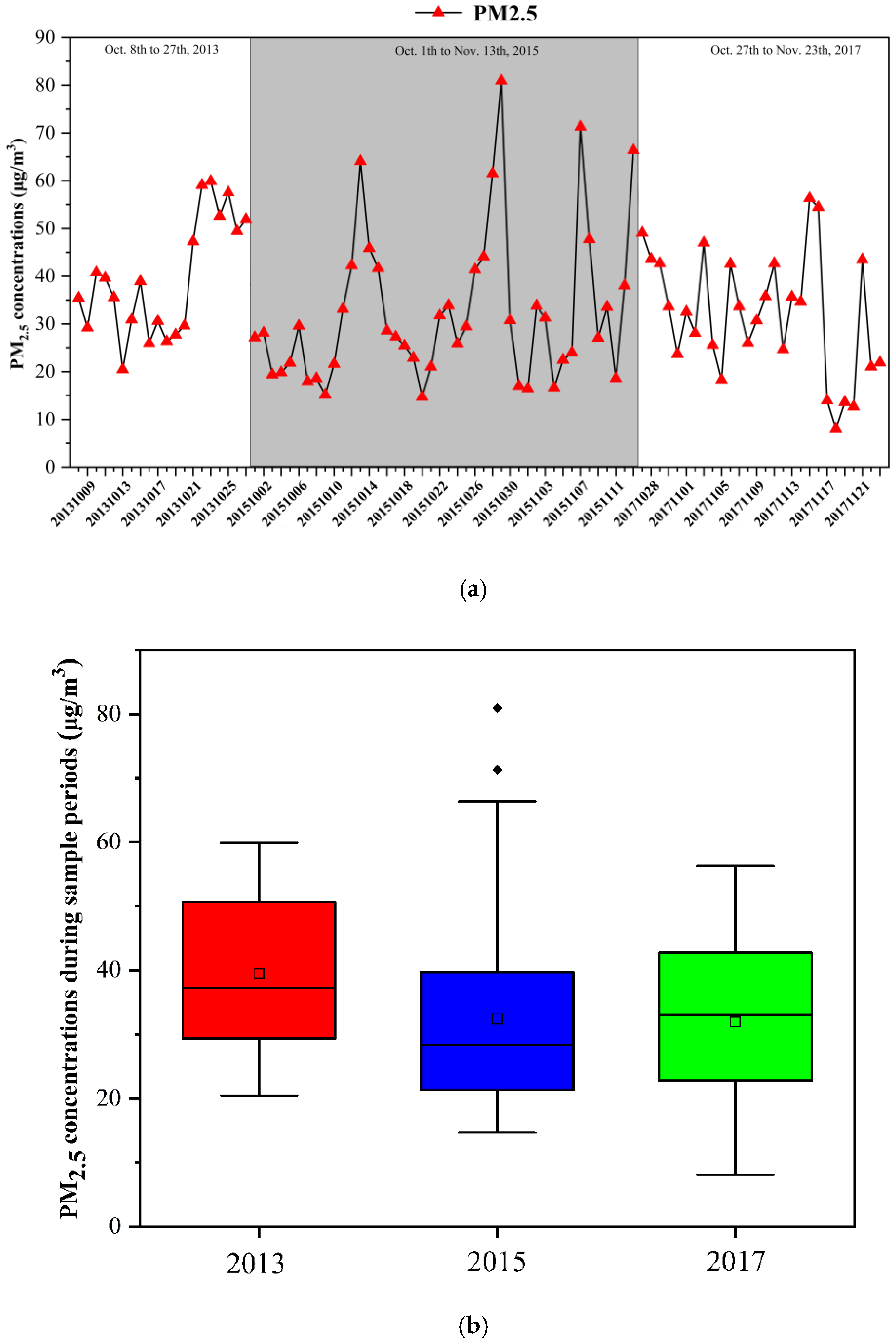
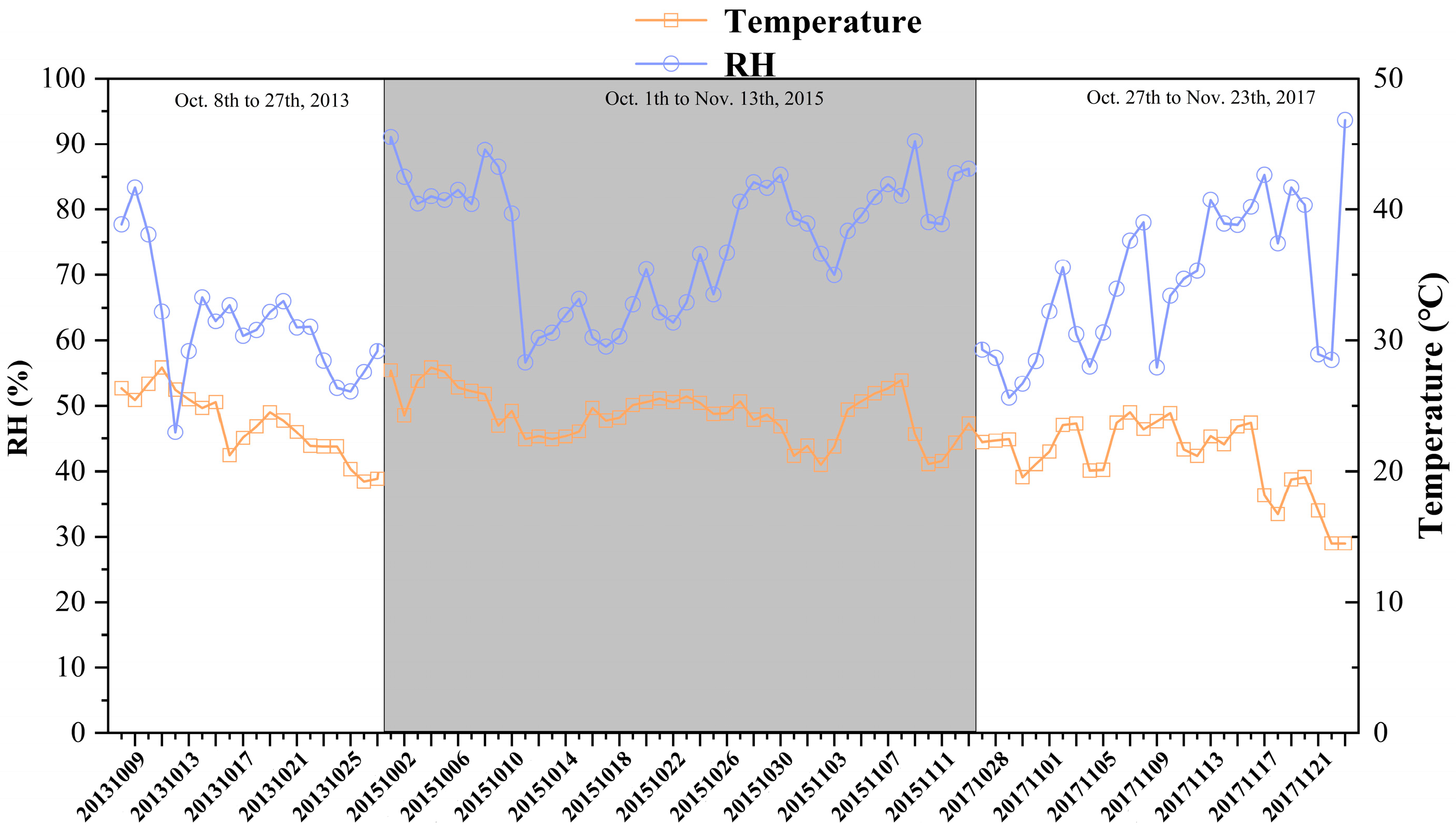
The daily and interannual variations in PM_2.5 concentrations during the autumn seasons of 2013, 2015, and 2017 in Xiamen are illustrated in Figure 2. Significant daily fluctuations in autumn PM_2.5 levels were observed in Figure 2a. Figure 3 reflects the daily temperature and relative humidity in Xiamen from the National Centers for Environmental Information (NCEI). Figure 2b shows a noticeable decline in average PM_2.5 concentration in autumn since 2013. However, the decrease in average PM_2.5 concentration between 2015 and 2017 was less pronounced than the decline observed after 2013. The average concentrations of PM_2.5 during autumn are illustrated in

Table 1. The mean concentrations of PM_2.5 and seven reconstructive components during sample periods in 2013, 2015, and 2017 in Xiamen (µg m⁻³).

Year	PM2.5	GM	OM	EC	TE	NO3−	SO42−	NH4+	Total	Others
2013	39.44	3.94	8.85	1.88	5.56	4.39	10.86	2.48	37.97	1.47
2015	32.50	8.39	7.64	2.24	0.81	2.02	7.38	3.77	32.24	0.26
2017	32.01	4.68	13.68	0.88	1.76	3.58	5.16	1.27	30.51	1.50

Note: GM means geological material; OM means organic matter; TE means trace elements; Total means the sum of seven reconstructive components; Others implies the value of PM_2.5 minus Total.

: 39.44 µg m⁻³ in 2013, 32.50 µg m⁻³ in 2015, and 32.01 µg m⁻³ in 2017. The autumn PM_2.5 concentrations in 2015 and 2017 met the secondary limit (35 μg/m³) of Chinese Ambient Air Quality Standards (GB 3095-2012) [34], demonstrating the effectiveness of local regulatory measures. For example, illegal biomass burning and firework displays had been banned for several years. Notably, during the 2017 BRICS Summit held in Xiamen, additional air quality measures were implemented, including the closure of heavily polluting factories, suspension of production in many factories, and restrictions on the shipment of hazardous chemical raw materials [35]. However, compared to the annual average PM_2.5 concentrations reported in the Xiamen Environmental Quality Bulletin (36 µg m⁻³ in 2013, 29 µg m⁻³ in 2015, and 27 µg m⁻³ in 217; https://sthjj.xm.gov.cn/), our autumn-specific data showed slightly higher values. This discrepancy likely arises from our observations being limited to the autumn seasons and not encompassing the entire year, as well as the concentration differences between manual and real-time monitoring [36].

To elucidate the chemical characteristics of PM_2.5, we employed a chemical mass reconstruction approach based on seven main components of PM_2.5: sulfate (SO₄²⁻), nitrate (NO₃⁻), ammonium (NH₄⁺), elemental carbon (EC), organic matter (OM, [OM] = 1.6[OC]), trace elements (TE, [TE] = [K] + [V] + [Mn] + [Co] + [Cu] + [Zn] + [As] + [Ba] + [Na]), and geological material (GM, [GM] = 2.20[Al] + 2.49[Si] + 1.63[Ca] + 1.94[Ti] + 2.52[Fe]) [9,37]. The reconstructed mass concentrations of PM_2.5 exhibited a strong linear correlation with the observed mass concentrations of PM_2.5 (Figure S1, r = 0.93, p < 0.001), validating the method’s robustness. The total reconstructed concentrations were 37.97 µg m⁻³ in 2013, 32.24 µg m⁻³ in 2015, and 30.51 µg m⁻³ in 2017 (Table 1), accounting for 96.3%, 99.2%, and 95.4% of the observed PM_2.5 mass, respectively (Figure 4). The daily variations of these reconstructed components can partly explain the fluctuations in PM_2.5 concentrations. For example, from 22 October to 25 October 2013, an increase in SO₄²⁻ concentration (Figure S2) was associated with higher PM_2.5 levels, with an average PM_2.5 concentration of 57.28 µg m⁻³ (Figure 2a). From 11 October to 15 October 2015, the concurrent rise in NH₄⁺, OM, and SO₄²⁻ concentrations (Figure S2) resulted in elevated PM_2.5 concentrations (45.41 µg m⁻³ on average) (Figure 2a). From 27 October to 29 October 2015, elevated concentrations of NH₄⁺, NO₃⁻, and SO₄²⁻ (Figure S2) led to an even higher average PM_2.5 concentration of 62.17 µg m⁻³ (Figure 2a). In contrast, from 17 November to 20 November 2017, decreases in all reconstructed components (Figure S2) resulted in a marked reduction in PM_2.5, with an average PM_2.5 concentration of only 12.08 µg m⁻³ (Figure 2a).

The proportions of reconstructed components exhibited significant interannual variations, reflecting changes in emission sources and atmospheric processes. GM, primarily associated with fugitive dust, showed a notable increase from 10% in 2013 to 25.8% in 2015, followed by a decrease to 14.4% in 2017 (Figure 4). This trend likely reflects dynamic fluctuations in the impact of fugitive dust, with the peak in 2015 corresponding to a surge in urban development projects [38]. Conversely, the decrease in GM proportion after 2015 may be associated with a reduction in construction activities. Additionally, the proportion of OM increased substantially from 23.5% in 2015 to 42.1% in 2017. In contrast, between 2013 and 2015, the proportion of OM increased by only 1.1% (Figure 4). This substantial increase in the OM from 2015 to 2017 could be attributed to several reasons: enhanced contributions from primary emissions (e.g., traffic and industrial sources), potential increase in secondary organic aerosol (SOA) formation driven by elevated volatile organic compound (VOCs) levels, and changes in meteorological conditions [39,40,41]. The proportions of reconstructed components within different PM_2.5 concentration ranges (0–25 µg/m³, 25–50 µg/m³, 50–75 µg/m³, and 75–100 µg/m³) are shown in Figure S3. As PM_2.5 concentrations rose, the proportion of OM and TE decreased, whereas the proportion of NO₃⁻ and NH₄⁺ increased. The observed rise in the fraction of water-soluble ions (SO₄²⁻ + NO₃⁻ + NH₄⁺) with increasing PM_2.5 concentrations highlights the importance of secondary pollutants, especially SO₄²⁻ and NO₃⁻, as major contributors to PM_2.5 pollution in Xiamen. This finding underscores the need for effective control of secondary aerosol precursors to mitigate air pollution.

TE, representing the total concentration of elements excluding minerals, decreased from 14.1% in 2013 to 2.5% in 2015 before rising modestly to 5.4% in 2017, potentially reflecting changes in industrial emissions and fuel combustion practices. A significant decline in both TE concentration and proportion had been observed since 2013, reflecting the effectiveness of stricter vehicle emission standards (GB18352.3-2005) [42] and power plant upgrades (https://www.hxpc.cn/hxdl/zjwm/fzlc/, accessed on 20 September 2024) in lowering TE levels. The water-soluble ions (SO₄²⁻ + NO₃⁻ + NH₄⁺) constituted a substantial fraction of PM_2.5, with proportions of 44.9%, 40.5%, and 30.8% in 2013, 2015, and 2017, respectively. SO₄²⁻ was the dominant ion, accounting for 27.5%, 22.7%, and 15.9% of PM_2.5 mass in the respective years. Considering the effect of shipping emissions on secondary sulfate concentrations in Xiamen [22], autumn PM_2.5 concentrations in 2013, 2015, and 2017 were likely influenced by ship emissions. EC, a tracer for combustion sources, showed the lowest percentage contribution, with proportions of 4.8%, 6.9%, and 2.7% in 2013, 2015, and 2017, respectively, indicating relatively stable contributions from fossil fuel combustion (Figure 4).

3.2. Source Apportionment of PM_2.5

3.2.1. PMF Model Setup and Validation

Before running the PMF model, the PM_2.5 was initially set as the total variable. Species with a signal-to-noise ratio (S/N) less than 0.5 (Ba and Cl⁻) were set as “Bad”, indicating that they were excluded from the PMF model. Those with 0.5 < S/N < 1 (Ti and Co) were set as “Weak”. The remaining species, with S/N > 1, were designated as “Strong”. The optimal solution with five factors was selected based on the distribution of residuals (Figure S4), which ranged between −3 and 3 for all species. The reconstructed PM_2.5 concentrations under this configuration accounted for 86.9%, 87.5%, and 92.4% of the observed values in 2013, 2015, and 2017, respectively, demonstrating the model’s robustness.

3.2.2. Source Profiles and Contributions

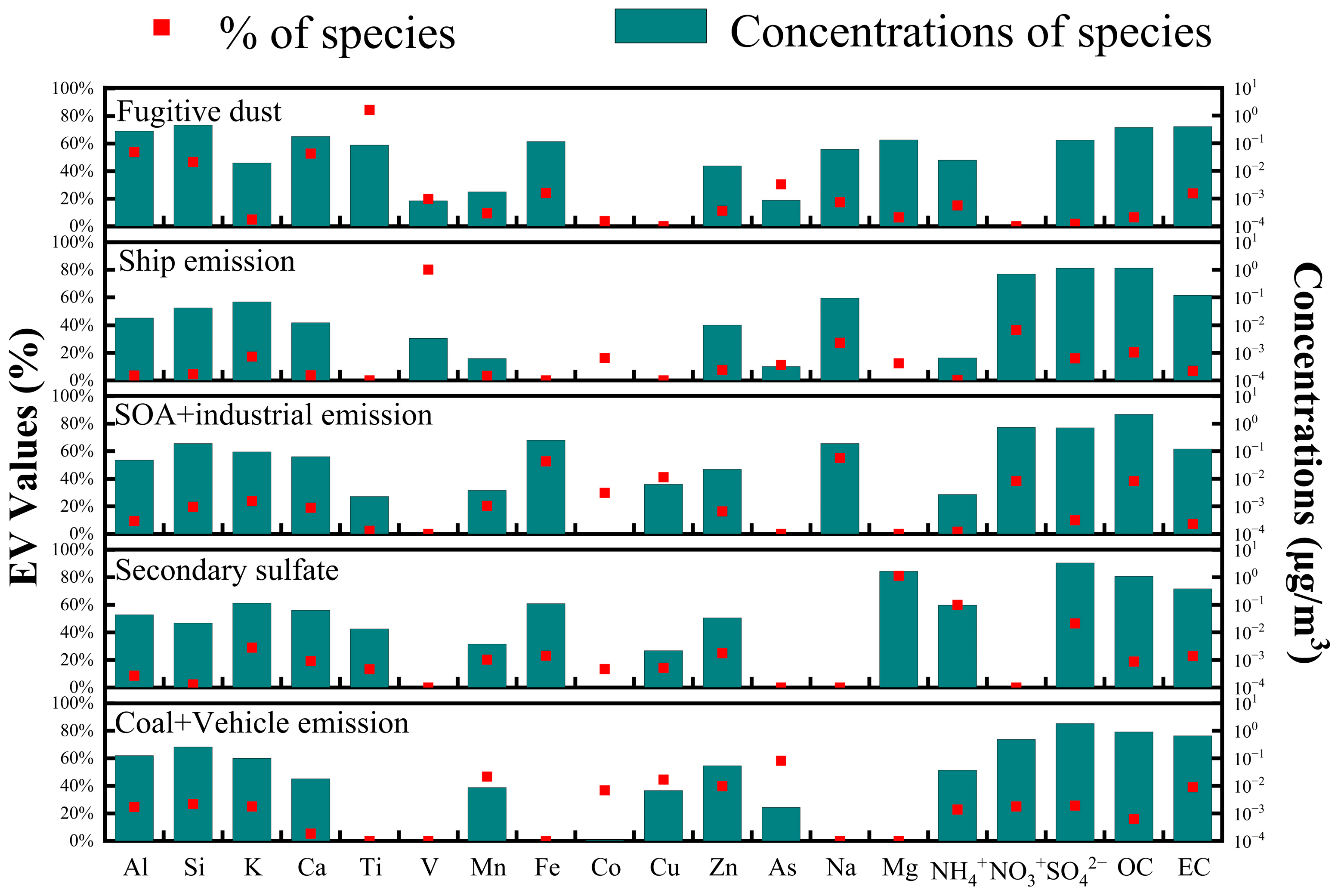
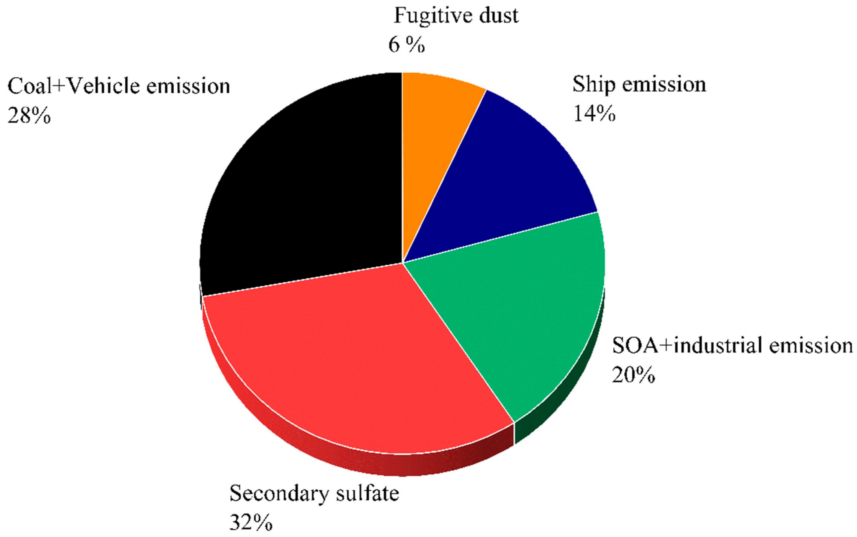
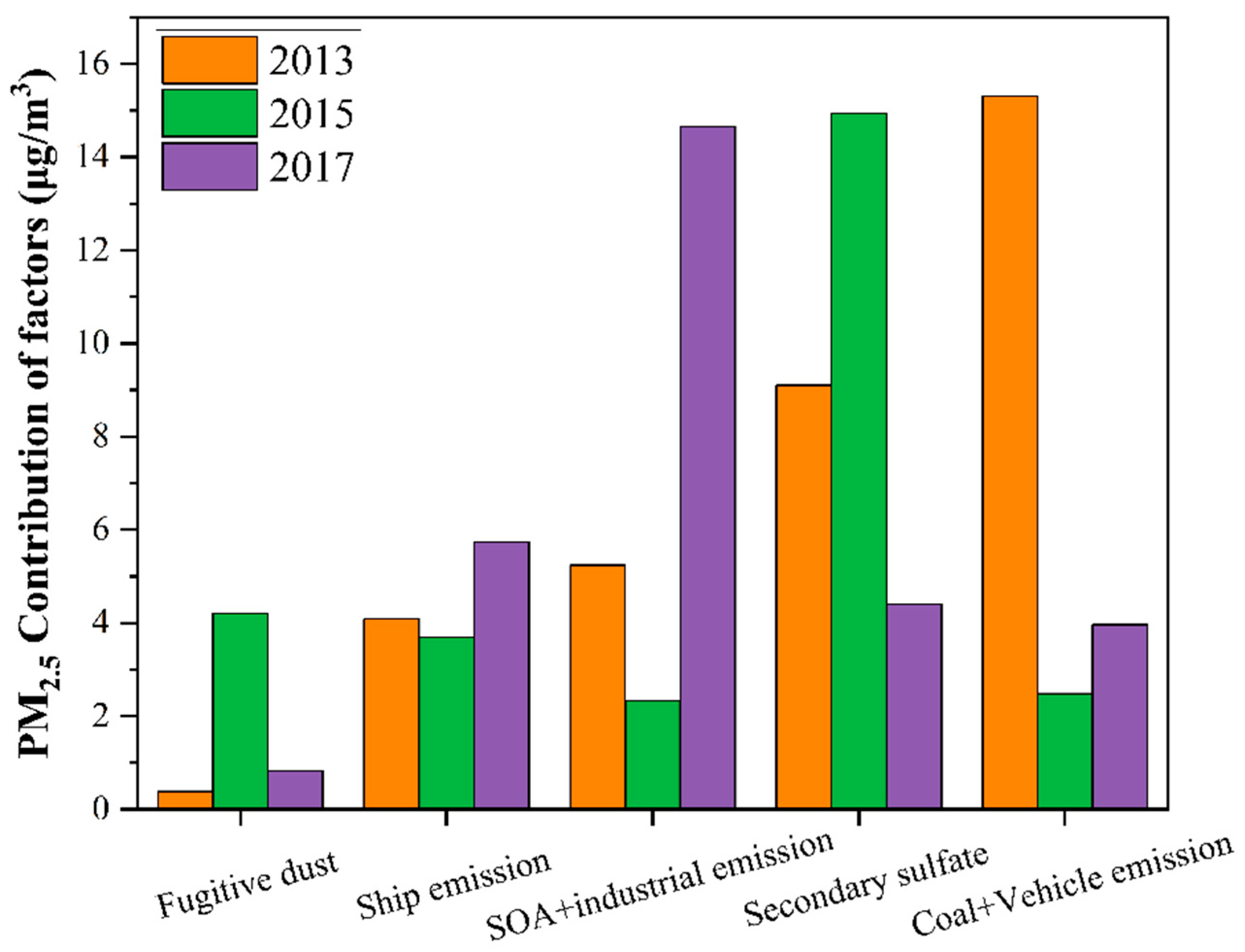
The source profiles and proportional contributions of the five factors are illustrated in Figure 5 and Figure 6, respectively. Temporal variations in the contributions of each source to PM_2.5 concentrations are presented in Figure 7.

Factor 1: Fugitive Dust

Factor 1 was identified as fugitive dust, supported by the high explained value (EV) of crustal-related elements, such as Al (55.3%), Si (47.9%), Ca (54.7%), and Ti (85.9%) (Figure 5) [43,44]. The elevated contribution of Ca and Ti suggests the influence of construction and resuspended road dust [45,46,47]. Factor 1 contributed minimally to the PM_2.5 levels in Xiamen, accounting for only 6% (Figure 6). This limited impact might be attributed to the city’s humid climate, characterized by higher relative humidity levels [23]. Despite its minimal overall contribution, fugitive dust exhibited significant interannual variability, with concentrations of 4.21 µg m⁻³ (2015) > 0.82 µg m⁻³ (2017) > 0.38 µg m⁻³ (2013) (Figure 7). This trend aligned with the variation in the proportion of GM components discussed in Section 3.1 and is primarily attributed to changes in construction activities rather than meteorological factors. For example, in 2015, Xiamen was simultaneously constructing Metro Lines 1 and 2, along with the ongoing urban village renovation projects [48,49].

Factor 2: Ship Emissions

Factor 2 was associated with ship emissions, characterized by its high EV of vanadium (V, 79.68%, Figure 5). Ship emissions accounted for 14% of the PM_2.5, a proportion higher than that observed in Qinhuangdao (3%, China) [50], Brindisi (6.1%, Italy) [51] and Busan (7%, South Korea) [52], close to in Shenzhen (17%, China) [53], but lower than in Hong Kong (19%, China) [53,54]. The concentration of ship-related remained relatively stable, with values of 4.09 µg m⁻³ (2013), 3.69 µg m⁻³ (2015), and 5.73 µg m⁻³ (2017) (Figure 7).

The presence of SO₄²⁻ in Factor 2 (Figure 5) indicates contributions from both primary particulate emissions and secondary sulfate formation driven by SO₂ oxidation catalyzed by V-containing particles [55]. To quantify the primary contributions of ships to PM_2.5, a V-based method was utilized as described by Agrawal et al. (2009) [56]. The following equation represents the methodology:

$${PM}_a={\displaystyle \frac{r\times V_a}{F_{v,HFO}}}$$

(5)

where ${PM}_a$ (µg m⁻³) represented the concentrations of primary PM_2.5 from shipping emissions; The $r$ value was 8205.8 ppm, suggesting the average ratio of PM_2.5 to the normalized V emission based on heavy fuel oil (HFO) burning experiments [56]; The $F_{v,HFO}$ value was 65.3 ppm, which denoted average V content of shipping HFO combustion. $V_a$ (µg m⁻³) served as the measured V concentrations in PM_2.5.

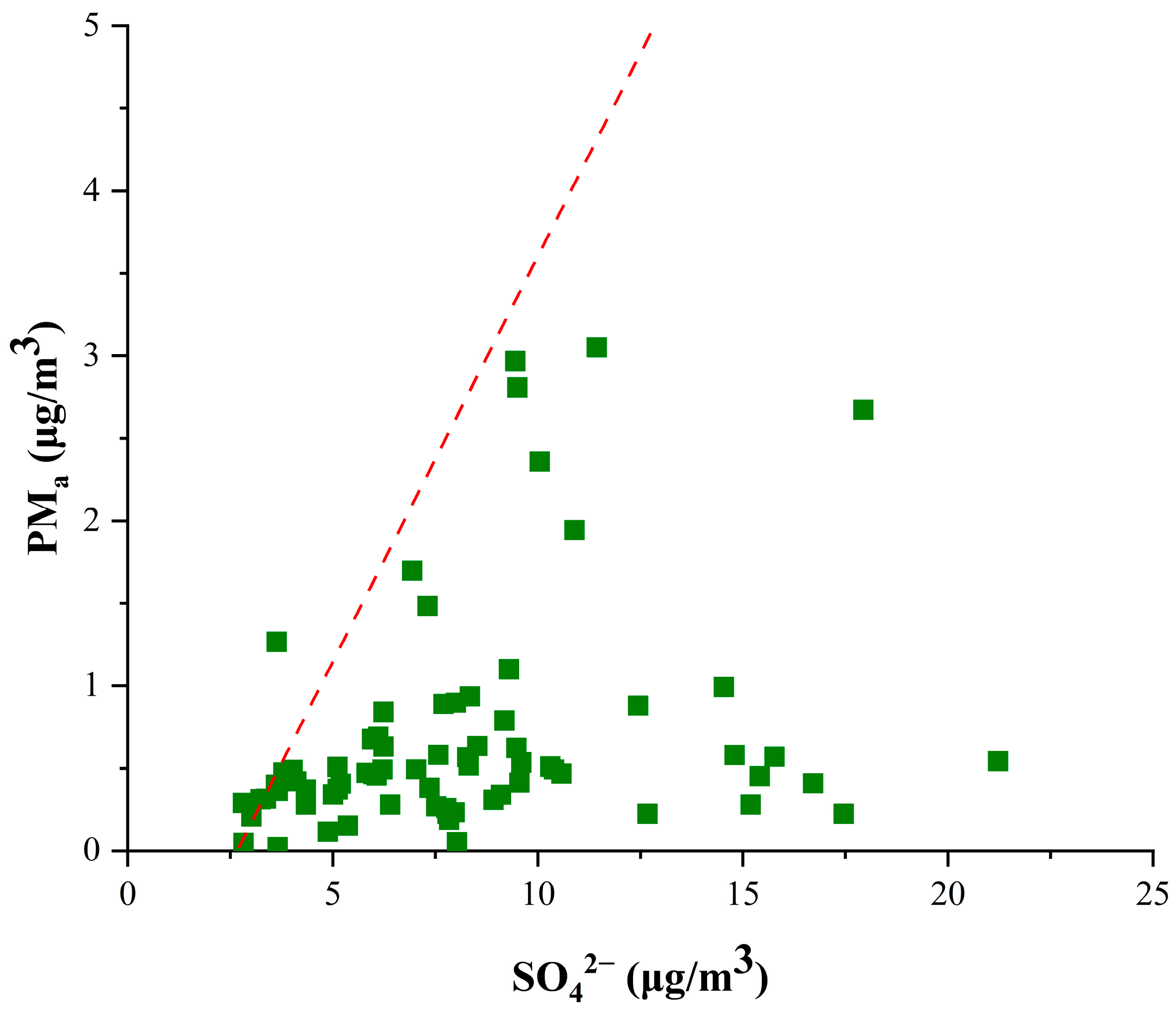
Using the V-based method, the concentrations of autumn primary PM_2.5 emissions from ships for the years 2013, 2015, and 2017 were calculated to range from 0.02 µg m⁻³ to 3.05 µg m⁻³, with an average value of 0.68 µg m⁻³. The proportion of ship-emitted primary PM_2.5 concentrations relative to the total PM_2.5 concentrations varied from 0.12% to 8.24%, with an average contribution of 2.00%, which was slightly lower than those reported in Brindisi (2.7%) [51] and Thessaloniki (2.9%) [57]. After obtaining the time series of primary PM_2.5 concentrations from ship emissions, we constructed scatter plots by combining ${PM}_a$ with the SO₄²⁻ concentrations (Figure 8). We utilized the slope of the upper edge line in the scatter plot to estimate the ratio between the concentration of primary PM_2.5 from ship emissions and the concentration of secondary sulfates [55]. A slope of 0.5 indicated that each 1.00 µg m⁻³ of primary PM_2.5 emitted by ships corresponded to an emission of 2.00 µg m⁻³ of secondary sulfates. The result surpassed the concentrations of SO₄²⁻ observed in other cities, such as Thessaloniki (0.56 µg m⁻³) and Seattle (0.83 µg m⁻³) [55,57]. The reason was that China did not enforce the low-sulfur (<0.5%) fuel oil (LSFO) policy for vessels in the Domestic Emission Control Area (DECA) until 2019. We then computed the total concentration of ship emissions using the V-based method, which incorporated both primary PM_2.5 and estimated SO₄²⁻. Compared with the PM_2.5 contributions from ship emissions obtained using the PMF model, the V-based method generally produced lower values. However, a significant positive correlation was observed between the results of the two methods (Figure S5, r = 0.62, p < 0.001).

Factor 3: SOA and Industrial Emissions

Factor 3 was characterized by high loadings of heavy metal elements (Fe, Cu, Co) (Figure 5), indicating that Factor 3 was associated with industrial sources. The absence of local iron and steel industries suggests that the Fe identified in Factor 3 originated from remote sources, likely transported from northern regions (e.g., San’an Steel Plant and Sanming Steel Plant). Factor 3 also had a high loading of organic carbon (OC, 38.40%). To further explore the influence of Factor 3 on OC, we calculated the OC/EC ratios of all samples. The average OC/EC ratio was 4.45, exceeding the typical range of 2.00–2.20, which suggests the formation of secondary organic carbon (SOC) [22]. The SOC concentrations for each sample were calculated based on the formula SOC = OC − EC × (OC/EC)min [30]. The average SOC/OC ratio was 59.0%, close to the 60.2% proposed by Zhang et al. [58] for autumn in Xiamen, which supports substantial secondary formation and highlights SOC as a critical component of OC in Xiamen. In addition, Factor 3 exhibited the highest OC/EC ratio of 18.33 among all factors (Table S3), further validating its considerable impact on SOC. In addition, due to its low EV of EC and K, Factor 3 appeared to have minimal contribution from POC associated with biomass burning or vehicle exhaust emissions [37]. Therefore, we assumed that Factor 3 represented a combination of industrial emissions and SOA, contributing 20% to the PM_2.5 in Xiamen during autumn (Figure 6).

Significant interannual variability was observed in the contribution of Factor 3 to PM_2.5 concentrations, with levels in order as: 14.66 µg m⁻³ (2017) > 5.24 µg m⁻³ in 2013 > and 2.33 µg m⁻³ in 2015 (Figure 7). The contribution decreased notably from 2013 to 2015, then increased sharply in 2017 compared to 2015. This pattern of variation closely paralleled the interannual variation in SOC concentrations, which followed the sequence: 8.15 µg m⁻³ (2017) > 3.30 µg m⁻³ (2013) > 2.12 µg m⁻³ (2015) (Table S1).

Factor 3 showed a significant positive linear correlation with SOC (Figure S6, r = 0.80, p < 0.001). According to meteorological data from the National Centers for Environmental Information (NCEI) (https://www.ncei.noaa.gov/data/, accessed on 14 September 2024), the average temperatures in Xiamen were 23.57 °C, 24.31 °C, and 20.84 °C during the three sampling periods, respectively (

Table 2. The mean Temperature and Relative humidity during sample periods in 2013, 2015 and 2017 in Xiamen.

Year	Temperature (°C)	Relative Humidity (%)
2013	23.57	62.65
2015	24.31	75.59
2017	20.84	69.88

). As illustrated in Figure S7, a negative correlation was observed between SOC concentrations and temperatures (Figure S7, r = −0.33, p < 0.001). The lower temperatures during the 2017 sampling period contributed to a lower mixing layer height, which restricted pollutant dispersion and enhanced SOC formation [59], resulting in elevated SOC concentrations. Additionally, the average relative humidity (RH) levels during the sampling periods were 65.65% in 2013, 75.59% in 2015, and 69.88% in 2017 (Table 2). Figure S8 demonstrated that SOC concentrations also showed a negative correlation with RH levels (Figure S8, r = −0.31, p < 0.001). The reason might be that the higher RH in 2017 was less conducive to surface O3 formation [60,61], which is known to facilitate SOC production [22], thereby contributing to the lower SOC levels observed in 2015 compared to 2017 [62]. Additionally, the weakening in aerosol acidity due to higher RH diminished the role of acidity in enhancing SOC formation [62]. To summarize, the relatively low value of SOA + industrial emissions observed in the fall of 2015 was influenced to some extent by elevated temperature and relative humidity.

Factor 4: Secondary Sulfate

Factor 4 was identified as a secondary sulfate based on its high loadings of NH₄⁺ (EV = 77.29%) and SO₄²⁻ (EV = 45.32%) (Figure 5). Factor 4 accounted for 32% of the PM_2.5 concentration in Xiamen during autumn, representing the highest contribution among all identified sources (Figure 6).

The average concentrations of PM_2.5 attributable to secondary sulfate varied significantly across the years, with 14.94 µg m⁻³ in 2015, 9.10 µg m⁻³ in 2013, and 4.41 µg m⁻³ in 2017, indicating a change from an initial increase to a subsequent decrease (Figure 7). The higher average temperature (24.31 °C) and RH (75.59%) during the 2015 sampling period might contribute to the elevated levels of secondary sulfate observed in that year, as the oxidation rate of SO₂ tended to increase under elevated temperature and humidity conditions [63,64]. The reduction in the contribution of secondary sulfate to PM_2.5 in 2017 might be partially due to the ultra-low emission upgrades implemented at the Songyu coal power plant (Figure 1). These upgrades resulted in a significant decrease in the emission of precursor gases for sulfate (https://www.hxpc.cn/hxdl/zjwm/fzlc/A340102index_1.htm, accessed on 20 September 2024).

Factor 5: Coal Combustion and Vehicle Emissions

Factor 5 was identified as a combined source of coal combustion and vehicle emissions, represented by high EV for specific tracers: As (58.94%), Co (36.19%), and Mn (46.97%) (Figure 5) [65,66]. These elements are well-documented markers of coal combustion, particularly from power plants. Additionally, the high loadings of Cu (EV = 43.50%), Zn (EV = 39.57%), OC (EV = 15.88%), and EC (EV = 39.20%) in Factor 5 suggested significant contributions from vehicle emissions. Cu and Zn were primarily sourced from non-exhaust emissions, such as brake and tire wear [67,68,69]. OC and EC are typical tracers of fossil fuel combustion, including gasoline and diesel engines [8,70]. Therefore, Factor 5 was characterized as a mixed source of coal combustion and vehicle emissions (Coal + vehicle emissions).

Factor 5 contributed 28% to the total PM_2.5 concentration in Xiamen during autumn (Figure 6). The contribution exhibited a clear temporal trend: 15.31 µg m⁻³ (2013) > 3.96 µg m⁻³ (2017) > 2.49 µg m⁻³ (2015), demonstrating a marked decrease following 2013 (Figure 7). The significant reduction after 2013 can be attributed to two key factors:

(1) Coal Combustion Control: The implementation of advanced combustion technologies and pipeline construction at the Songyu coal power plant in 2015 (https://www.hxpc.cn/hxdl/zjwm/fzlc/, accessed on 20 September 2024) substantially reduced PM_2.5 emissions from coal combustion.

(2) Vehicle Emission Standards: The enforcement of the Limits and Measurement Methods for Emissions from Light-Duty Vehicles (IV) (GB18352.3-2005) in July 2013 led to significant improvements in vehicle emission controls, particularly for light-duty vehicles.

Despite these reductions, the slight increase in Factor 5 contributions in 2017 may reflect the growing number of vehicles in Xiamen, which partially offset the emission reductions achieved through regulatory measures. Particularly since 2011, the number of vehicles in Xiamen has been growing at an annual rate of nearly 20%. By 2015, the number of vehicles in the city had reached 1.2 million [71,72]. This highlights the need for continued efforts to balance urban development with air quality management.

3.3. Backward Trajectory Cluster and PSCF Analysis

3.3.1. Backward Trajectory Clustering

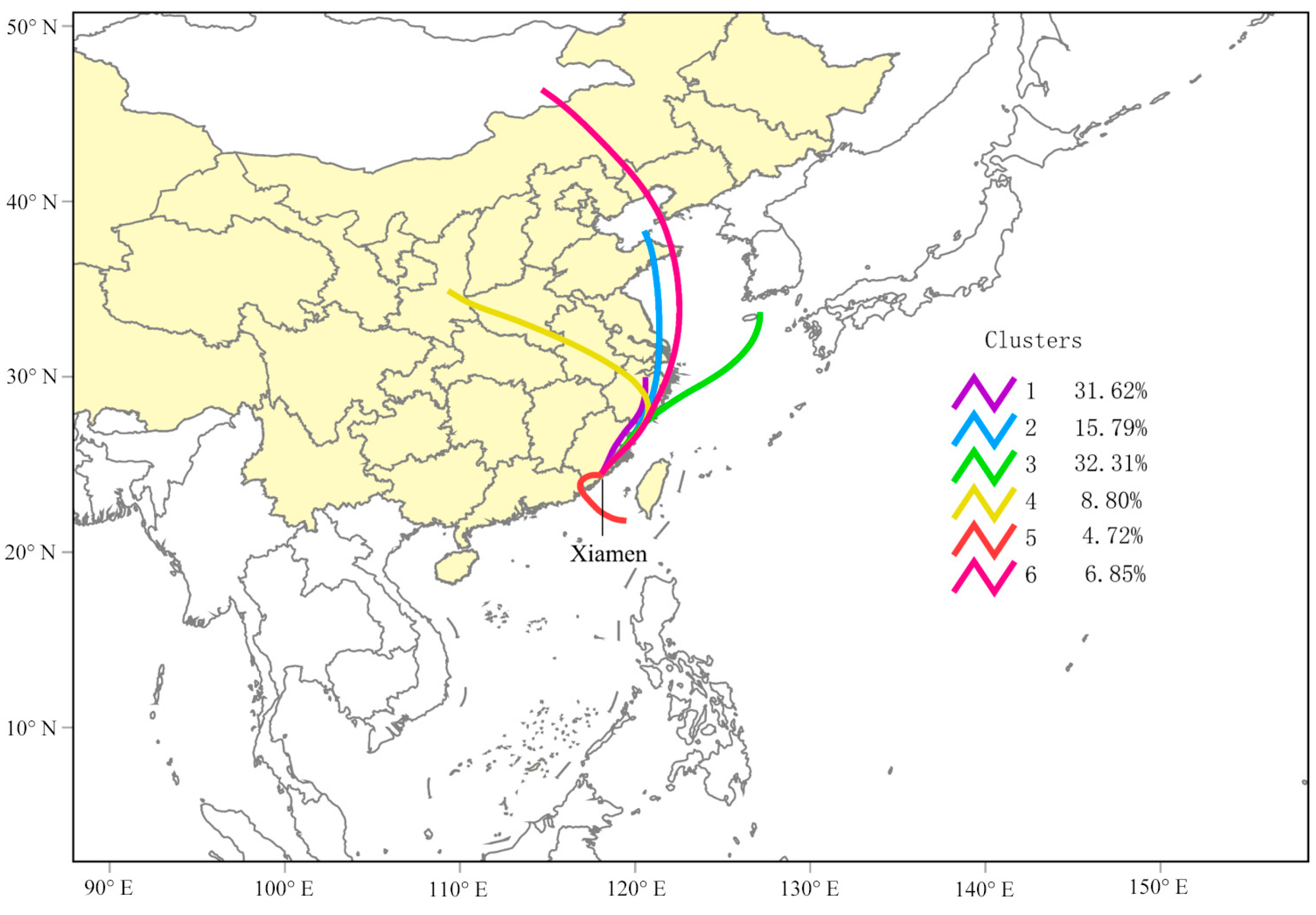
Figure 9 illustrates that the 72-h backward trajectories for Xiamen during the autumn seasons of 2013, 2015, and 2017 were categorized into six clusters. These clusters represent distinct air mass transport pathways influencing PM_2.5 concentrations in Xiamen:

Cluster 1 (31.62%): Originating from the northern Zhejiang Province, this cluster traversed northeastern Fujian Province, reflecting regional transport from the Yangtze River Delta region.

Cluster 2 (15.79%): This cluster originated over the Bohai Sea, traversing the Shandong Peninsula, the Yellow Sea, the Yangtze River Delta, and the eastern part of Zhejiang Province before reaching the northern part of Fujian Province. This cluster highlights the potential influence of industrial and maritime emissions from North China.

Cluster 3 (32.31%): Originating from the northeastern sea of Jeju Island, South Korea, this cluster crossed the East Sea before ultimately passing over the eastern coastal region of Fujian Province, indicating the potential for transboundary pollution transport.

Cluster 4 (8.80%): Starting in central Shanxi Province, this cluster moved southeastward through Henan, Anhui, and Zhejiang Provinces before following the eastern coastline of Fujian Province. Its pathway suggests contributions from inland industrial and coal combustion sources.

Cluster 5 (4.72%): Originating over the southwestern sea surface of Taiwan Province, this cluster propagated northwestward to the Guangdong-Fujian border and then northeastward through southern Fujian Province, reflecting potential contributions from maritime and southern regional sources.

Cluster 6 (6.85%): Characterized by the longest transmission distance, this cluster originated in eastern Mongolia and traversed Inner Mongolia, western Liaoning, the Liaodong Peninsula, and the Shandong Peninsula. After crossing the Yellow Sea, the cluster continued to follow the eastern coastline of Zhejiang and Fujian Province. Its trajectory underscores the potential for long-range transport of pollutants from northern China and Mongolia.

Overall, the majority of air masses affecting Xiamen during autumn originated from the northern and northeastern quadrants, highlighting the significant influence of regional transport on local PM_2.5 levels. Figure S9 displays the backward trajectories separately for autumn in 2013, 2015, and 2017. While all three years showed that air masses affecting Xiamen mainly came from the north and northeast, the specific geographic origins of these air masses varied between years.

3.3.2. PSCF Analysis

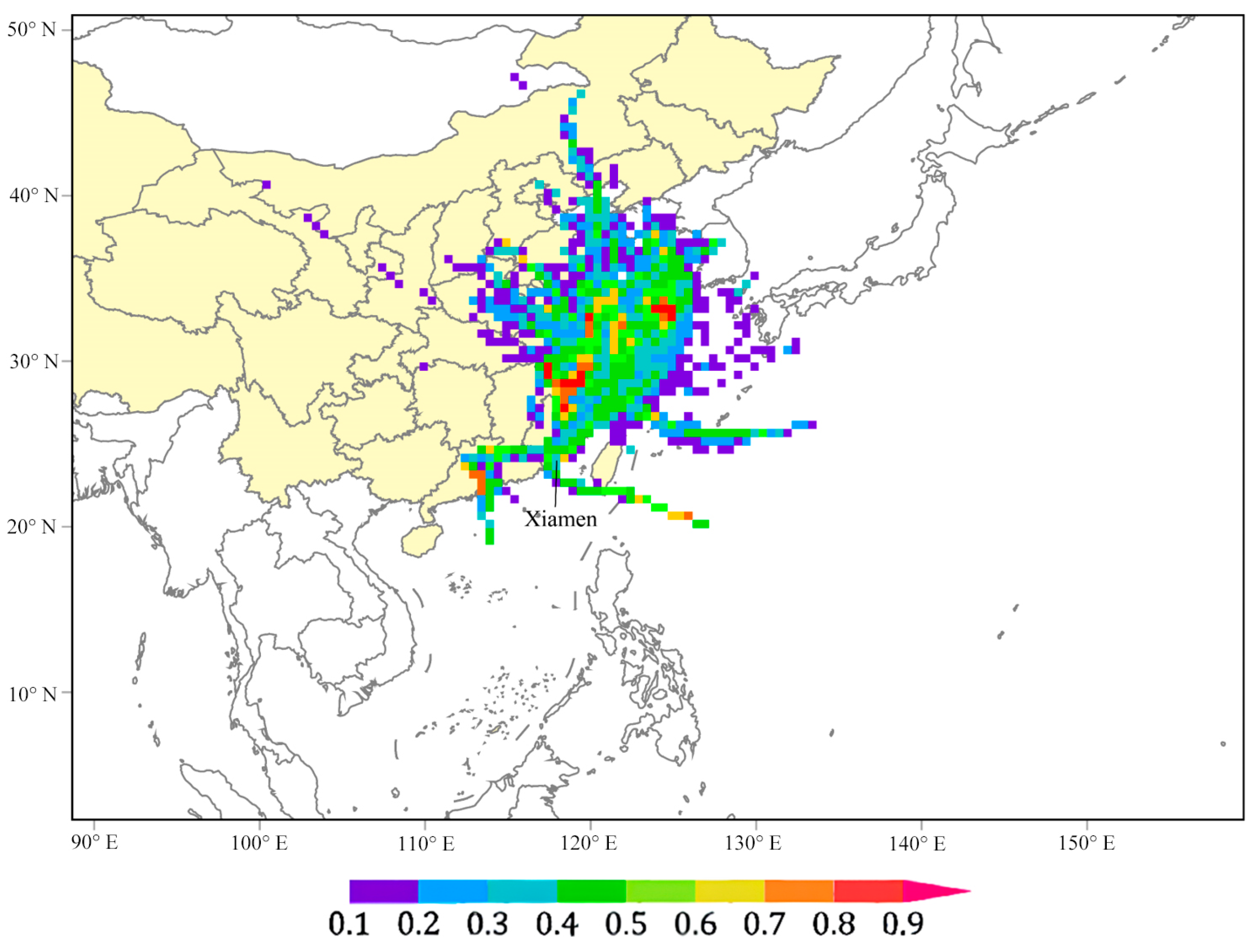
The PSCF analysis was conducted using a criterion value of PSCF of 35 µg m⁻³, based on China’s National Ambient Air Quality Standard (GB 3095-2012). Figure 10 presents the spatial distribution of WPSCF values for PM_2.5 in Xiamen during the autumn seasons. High WPSCF values were observed in the following regions:

• Pearl River Delta, a major industrial and urban agglomeration in southern China.
• Areas spanning northern Fujian to the Yangtze River Delta, indicating contributions from industrial and urban emissions in these regions.
• The maritime area between Shanghai and Jeju Island, suggesting the influence of ship emissions and transboundary transport.

These findings align closely with the cluster analysis, confirming that the primary potential sources of autumn PM_2.5 in Xiamen are located north and northeast of the city, including industrial zones and maritime regions affected by shipping activities. As shown in Figure S10, the WPSCF results for 2013, 2015, and 2017 are presented, respectively, which were largely consistent with the outcomes derived from the cluster analysis. It can be observed that in 2013 the potential sources of autumn PM_2.5 in Xiamen were more extensively distributed over inland regions, particularly in northern Fujian Province, such as the urban areas of Nanping and Sanming. By contrast, in 2015 and 2017 the potential source areas were more associated with marine regions. Considering the corresponding mean PM_2.5 concentrations of 39.44 µg m⁻³ in 2013, 32.50 µg m⁻³ in 2015, and 32.01 µg m⁻³ in 2017 (Table 1), these results suggest that long-range transport of PM_2.5 from inland, especially from urban areas, contributed to the elevated PM_2.5 levels in Xiamen in 2013. The consistency between the WPSCF and clustering results underscores the importance of regional cooperation in addressing PM_2.5 pollution in coastal cities like Xiamen.

4. Conclusions

This study investigated the sources of PM_2.5 and interannual variations in Xiamen from autumn 2013 to 2017. Average PM_2.5 concentrations declined from 39.44 µg m⁻³ (2013) to 32.01 µg m⁻³ (2017), with dominant components shifting from sulfate (SO₄²⁻, 27.5%) to GM (25.8%) and OM (42.1%). The PMF model identified five sources: secondary sulfate (32%), coal and vehicle emissions (28%), SOA and industrial emissions (20%), ship emissions (14%), and fugitive dust (6%). Source contributions varied annually due to anthropogenic activities and meteorological conditions. Fugitive dust peaked in 2015 due to construction activities, while SOA and secondary sulfate were influenced by temperature and humidity. Coal and vehicle emissions declined after 2013, primarily due to stricter vehicle standards and upgrades at power plants. Ship emissions remained stable. The above conclusion regarding the interannual variation of PM_2.5 emission factors in Xiamen is the primary focus of our study, which differs from previous studies. Backward trajectory clustering and PSCF analyses indicated that primary PM_2.5 sources were located north and northeast of Xiamen, including industrial zones and maritime areas.

Study limitations included sampling inconsistencies, the incompleteness of the measured species, and the fact that data were only collected during the autumn season; however, the analysis of interannual variations provided three novel insights. First, the longitudinal nature of the dataset enabled the identification of stable trends in emission source contributions, most notably, the persistent 14% contribution of ship emissions to PM_2.5 in a major port city. This finding provided foundational evidence for policymaking in the maritime sector, which is increasingly urgent as shipping accounts for nearly 90% of global trade and continues to grow [73]. Second, the integration of PMF with Potential Source Contribution Function (PSCF) results revealed that approximately 32% of PM_2.5 was transported from distant regions, a result with important implications for transboundary air pollution governance. Third, the study’s temporal coverage—capturing two key regulatory milestones in 2013 and 2015—enabled a robust assessment of the impacts of vehicle emission standards and power plant upgrades. The nearly 80% decline in coal- and vehicle-related PM_2.5 over a four-year period underscored the effectiveness of these interventions. Furthermore, the temperature-driven increase in secondary organic aerosols (SOA) observed between 2015 and 2017 provided mechanistic insight into why coastal cities continue to struggle with meeting WHO air quality targets, despite stringent emission controls. All in all, this study enhances understanding of PM_2.5 dynamics in coastal cities and supports targeted air quality management.

References

1. Zhu, T.; Liu, Y.; Xu, S.; Dong, G.; Huang, C.; Sang, N.; Zhang, Y.; Su, G.; Chen, J.; Gong, J.; et al. Advances and perspectives in environmental health research in China. Front. Environ. Sci. Eng. 2024, 18, 76. [Google Scholar] [CrossRef]
2. Darrow, L.A.; Klein, M.; Flanders, W.D.; Mulholland, J.A.; Tolbert, P.E.; Strickland, M.J. Air pollution and acute respiratory infections among children 0–4 years of age: An 18-year time-series study. Am. J. Epidemiol. 2014, 180, 968–977. [Google Scholar] [CrossRef] [PubMed]
3. Huang, C.; Nichols, C.; Liu, Y.; Zhang, Y.; Liu, X.; Gao, S.; Li, Z.; Ren, A. Ambient air pollution and adverse birth outcomes: A natural experiment study. Popul. Health Metr. 2015, 13, 17. [Google Scholar] [CrossRef] [PubMed]
4. Schraufnagel, D.E.; Balmes, J.R.; Cowl, C.T.; De Matteis, S.; Jung, S.-H.; Mortimer, K.; Perez-Padilla, R.; Rice, M.B.; Riojas-Rodriguez, H.; Sood, A.; et al. Air Pollution and Noncommunicable Diseases: A Review by the Forum of International Respiratory Societies’ Environmental Committee, Part 2: Air Pollution and Organ Systems. Chest 2019, 155, 417–426. [Google Scholar] [CrossRef]
5. Intergovernmental Panel on Climate Change. Working Group I Contribution to the Fifth Assessment Report of the Intergovernmental Panel on Climate Change. In Climate Change 2013—The Physical Science Basis; Cambridge University Press: Cambridge, MA, USA, 2014. [Google Scholar]
6. Zhou, H.; Yue, X.; Dai, H.; Geng, G.; Yuan, W.; Chen, J.; Shen, G.; Zhang, T.; Zhu, J.; Liao, H. Recovery of ecosystem productivity in China due to the Clean Air Action plan. Nat. Geosci. 2024, 17, 1233–1239. [Google Scholar] [CrossRef]
7. Matson, P.; Kathleen, A.L.; Hall, S.J. The Globalization of Nitrogen Deposition: Consequences for Terrestrial Ecosystems. Ambio 2002, 31, 113–119. [Google Scholar] [CrossRef] [PubMed]
8. Liu, B.; Wu, J.; Zhang, J.; Wang, L.; Yang, J.; Liang, D.; Dai, Q.; Bi, X.; Feng, Y.; Zhang, Y.; et al. Characterization and source apportionment of PM2.5 based on error estimation from EPA PMF 5.0 model at a medium city in China. Environ. Pollut. 2017, 222, 10–22. [Google Scholar] [CrossRef]
9. Zhang, N.; Zhuang, M.; Tian, J.; Tian, P.; Zhang, J.; Wang, Q.; Zhou, Y.; Huang, R.; Zhu, C.; Zhang, X.; et al. Development of source profiles and their application in source apportionment of PM2.5 in Xiamen, China. Front. Environ. Sci. Eng. 2016, 10, 17. [Google Scholar] [CrossRef]
10. Zhang, Q.; Meng, X.; Shi, S.; Kan, L.; Chen, R.; Kan, H. Overview of particulate air pollution and human health in China: Evidence, challenges, and opportunities. Innovation 2022, 3, 100312. [Google Scholar] [CrossRef]
11. Huang, R.J.; Zhang, Y.; Bozzetti, C.; Ho, K.F.; Cao, J.J.; Han, Y.; Daellenbach, K.R.; Slowik, J.G.; Platt, S.M.; Canonaco, F.; et al. High secondary aerosol contribution to particulate pollution during haze events in China. Nature 2014, 514, 218–222. [Google Scholar] [CrossRef]
12. Dai, X.; Zhang, Z.; Jin, Y.; Niu, Y.; Cao, H.; Liang, X.; Chen, L.; Wang, J.; Peng, X. Solution-processed, high-performance light-emitting diodes based on quantum dots. Nature 2014, 515, 96–99. [Google Scholar] [CrossRef]
13. Gu, J.; Bai, Z.; Li, W.; Wu, L.; Liu, A.; Dong, H.; Xie, Y. Chemical composition of PM2.5 during winter in Tianjin, China. Particuology 2011, 9, 215–221. [Google Scholar] [CrossRef]
14. Kang, H.; Zhu, B.; Su, J.; Wang, H.; Zhang, Q.; Wang, F. Analysis of a long-lasting haze episode in Nanjing, China. Atmos. Res. 2013, 120–121, 78–87. [Google Scholar] [CrossRef]
15. Cheng, J.; Su, J.; Cui, T.; Li, X.; Dong, X.; Sun, F.; Yang, Y.; Tong, D.; Zheng, Y.; Li, Y.; et al. Dominant role of emission reduction in PM2.5 air quality improvement in Beijing during 2013–2017: A model-based decomposition analysis. Atmos. Chem. Phys. 2019, 19, 6125–6146. [Google Scholar] [CrossRef]
16. Zhao, B.; Wang, S.X.; Hao, J.M. Challenges and perspectives of air pollution control in China. Front. Environ. Sci. Eng. 2024, 18, 68. [Google Scholar] [CrossRef]
17. Ting, F.; Chen, T.; Li, M.; Chi, J.; Tang, H.; Zhang, T.; Li, H. Discrimination of the pollution grade of metal elements in atmospherically deposited particulate matter via laser-induced breakdown spectroscopy combined with machine learning method. Chemom. Intell. Lab. Syst. 2022, 231, 104691. [Google Scholar] [CrossRef]
18. Zhu, Y.; Huang, L.; Li, J.; Ying, Q.; Zhang, H.; Liu, X.; Liao, H.; Li, N.; Liu, Z.; Mao, Y. Sources of particulate matter in China: Insights from source apportionment studies published in 1987–2017. Environ. Int. 2018, 115, 343–357. [Google Scholar] [CrossRef] [PubMed]
19. Pai, S.J.; Carter, T.S.; Heald, C.L.; Kroll, J.H. Updated World Health Organization Air Quality Guidelines Highlight the Importance of Non-anthropogenic PM2.5. Environ. Sci. Technol. Lett. 2022, 9, 501–506. [Google Scholar] [CrossRef]
20. Wang, S.; Hu, G.; Yan, Y.; Wang, S.; Yu, R.; Cui, J. Source apportionment of metal elements in PM2.5 in a coastal city in Southeast China: Combined Pb-Sr-Nd isotopes with PMF method. Atmos. Environ. 2019, 198, 302–312. [Google Scholar] [CrossRef]
21. Wu, S.-P.; Cai, M.-J.; Xu, C.; Zhang, N.; Zhou, J.-B.; Yan, J.-P.; Schwab, J.J.; Yuan, C.-S. Chemical nature of PM2.5 and PM10 in the coastal urban Xiamen, China: Insights into the impacts of shipping emissions and health risk. Atmos. Environ. 2020, 227, 117383. [Google Scholar] [CrossRef]
22. Wu, S.-P.; Xu, C.; Dai, L.-H.; Zhang, N.; Wei, Y.; Gao, Y.; Yan, J.-P.; Schwab, J.J. Source Apportionment of PM2.5 at Urban and Suburban Sites in a Port City of Southeastern China. Aerosol Air Qual. Res. 2019, 19, 2017–2031. [Google Scholar] [CrossRef]
23. Taghvaee, S.; Sowlat, M.H.; Mousavi, A.; Hassanvand, M.S.; Yunesian, M.; Naddafi, K.; Sioutas, C. Source apportionment of ambient PM2.5 in two locations in central Tehran using the Positive Matrix Factorization (PMF) model. Sci. Total Environ. 2018, 628–629, 672–686. [Google Scholar] [CrossRef]
24. Paatero, P.; Tapper, U. Positive matrix factorization: A non-negative factor model with optimal utilization of error estimates of data values. Environmetrics 1994, 5, 111–126. [Google Scholar] [CrossRef]
25. Paatero, P. End User’s Guide to Multilinear Engine Applications; University of Helsinki: Helsinki, Finland, 2007. [Google Scholar]
26. Brown, S.G.; Eberly, S.; Paatero, P.; Norris, G.A. Methods for estimating uncertainty in PMF solutions: Examples with ambient air and water quality data and guidance on reporting PMF results. Sci. Total Environ. 2015, 518–519, 626–635. [Google Scholar] [CrossRef]
27. Seibert, P.; Frank, A. Source-receptor matrix calculation with a Lagrangian particle dispersion model in backward mode. Atmos. Chem. Phys. 2004, 4, 51–63. [Google Scholar] [CrossRef]
28. Wang, Y.Q.; Zhang, X.Y.; Draxler, R.R. TrajStat: GIS-based software that uses various trajectory statistical analysis methods to identify potential sources from long-term air pollution measurement data. Environ. Model. Softw. 2009, 24, 938–939. [Google Scholar] [CrossRef]
29. Wang, Y. An Open Source Software Suite for Multi-Dimensional Meteorological Data Computation and Visualisation. J. Open Res. Softw. 2019, 7, 21. [Google Scholar] [CrossRef]
30. Xu, L.; Chen, J.; Yang, L.; Niu, Z.; Tong, L.; Yin, L.; Chen, Y. Characteristics and sources of atmospheric mercury speciation in a coastal city, Xiamen, China. Chemosphere 2015, 119, 530–539. [Google Scholar] [CrossRef] [PubMed]
31. Markou, M.T.; Kassomenos, P. Cluster analysis of five years of back trajectories arriving in Athens, Greece. Atmos. Res. 2010, 98, 438–457. [Google Scholar] [CrossRef]
32. Zeng, Y.; Hopke, P.K. A study of the sources of acid precipitation in Ontario, Canada. Atmos. Environ. (1967) 1989, 23, 1499–1509. [Google Scholar] [CrossRef]
33. Polissar, A.V.; Hopke, P.K.; Harris, J.M. Source regions for atmospheric aerosol measured at Barrow, Alaska. Environ. Sci. Technol. 2001, 35, 4214–4226. [Google Scholar] [CrossRef]
34. GB 3095-2012; Ambient Air Quality Standards. Ministry of Environmental Protection of the People’s Republic of China: Beijing, China, 2012.
35. Wang, S.; Yan, Y.; Yu, R.; Shen, H.; Hu, G.; Wang, S. Influence of pollution reduction interventions on atmospheric PM2.5: A case study from the 2017 Xiamen. Atmos. Pollut. Res. 2021, 12, 101137. [Google Scholar] [CrossRef]
36. Lee, J.H.; Hopke, P.K.; Holsen, T.M.; Polissar, A.V. Evaluation of continuous and filter-based methods for measuring PM2.5 mass concentration. Aerosol Sci. Technol. 2005, 39, 290–303. [Google Scholar] [CrossRef]
37. Xu, H.; Guinot, B.; Shen, Z.; Ho, K.; Niu, X.; Xiao, S.; Huang, R.-J.; Cao, J. Characteristics of Organic and Elemental Carbon in PM2.5 and PM0.25 in Indoor and Outdoor Environments of a Middle School: Secondary Formation of Organic Carbon and Sources Identification. Atmosphere 2015, 6, 361–379. [Google Scholar] [CrossRef]
38. Azarmi, F.; Kumar, P.; Marsh, D.; Fuller, G. Assessment of the long-term impacts of PM10 and PM2.5 particles from construction works on surrounding areas. Environ. Sci. Process. Impacts 2016, 18, 208–221. [Google Scholar] [CrossRef] [PubMed]
39. Chaturvedi, S.; Kumar, A.; Singh, V.; Chakraborty, B.; Kumar, R.; Min, L. Recent Advancement in Organic Aerosol Understanding: A Review of Their Sources, Formation, and Health Impacts. Water Air Soil Pollut. 2023, 234, 750. [Google Scholar] [CrossRef]
40. Feng, J.; Chan, C.K.; Fang, M.; Hu, M.; He, L.; Tang, X. Impact of meteorology and energy structure on solvent extractable organic compounds of PM2.5 in Beijing, China. Chemosphere 2005, 61, 623–632. [Google Scholar] [CrossRef]
41. Tian, Y.; Liu, X.; Huo, R.; Shi, Z.; Sun, Y.; Feng, Y.; Harrison, R.M. Organic compound source profiles of PM2.5 from traffic emissions, coal combustion, industrial processes and dust. Chemosphere 2021, 278, 130429. [Google Scholar] [CrossRef]
42. GB18352.3-2005; Limits and Measurement Methods for Emissions from Light-Duty Vehicles (III, IV). Ministry of Environmental Protection of the People’s Republic of China: Beijing, China, 2005.
43. Liu, B.; Song, N.; Dai, Q.; Mei, R.; Sui, B.; Bi, X.; Feng, Y. Chemical composition and source apportionment of ambient PM2.5 during the non-heating period in Taian, China. Atmos. Res. 2016, 170, 23–33. [Google Scholar] [CrossRef]
44. Manousakas, M.; Papaefthymiou, H.; Diapouli, E.; Migliori, A.; Karydas, A.G.; Bogdanovic-Radovic, I.; Eleftheriadis, K. Assessment of PM2.5 sources and their corresponding level of uncertainty in a coastal urban area using EPA PMF 5.0 enhanced diagnostics. Sci. Total Environ. 2017, 574, 155–164. [Google Scholar] [CrossRef]
45. Xue, Y.-H.; Wu, J.-H.; Feng, Y.-C.; Dai, L.; Bi, X.-H.; Li, X.; Zhu, T.; Tang, S.-B.; Chen, M.-F. Source Characterization and Apportionment of PM10 in Panzhihua, China. Aerosol Air Qual. Res. 2010, 10, 367–377. [Google Scholar] [CrossRef]
46. Peltier, R.E.; Cromar, K.R.; Ma, Y.; Fan, Z.-H.; Lippmann, M. Spatial and seasonal distribution of aerosol chemical components in New York City: (2) Road dust and other tracers of traffic-generated air pollution. J. Expo. Sci. Environ. Epidemiol. 2011, 21, 484–494. [Google Scholar] [CrossRef] [PubMed]
47. Pant, P.; Harrison, R.M. Estimation of the contribution of road traffic emissions to particulate matter concentrations from field measurements: A review. Atmos. Environ. 2013, 77, 78–97. [Google Scholar] [CrossRef]
48. Huang, G.; Wang, H.; Xu, D. Understanding the complementary effect of bike-sharing on public transit: A case study of subway line expansion in Xiamen, China. J. Transp. Geogr. 2024, 121, 104021. [Google Scholar] [CrossRef]
49. Tian, L.; Yao, Z.; Fan, C.; Zhou, L. A systems approach to enabling affordable housing for migrants through upgrading Chengzhongcun: A case of Xiamen. Cities 2020, 105, 102186. [Google Scholar] [CrossRef]
50. Lang, J.; Zhou, Y.; Chen, D.; Xing, X.; Wei, L.; Wang, X.; Zhao, N.; Zhang, Y.; Guo, X.; Han, L.; et al. Investigating the contribution of shipping emissions to atmospheric PM2.5 using a combined source apportionment approach. Environ. Pollut. 2017, 229, 557–566. [Google Scholar] [CrossRef]
51. Cesari, R.; Genga, A.; Buccolieri, R.; Di Sabatino, S.; Siciliano, M.; Siciliano, T.; Dinoi, A.; Maurizi, A.; Ielpo, P. Combining Chemical Composition Data and Numerical Modelling for the Assessment of Air Quality in a Mediterranean Port City. Appl. Sci. 2021, 11, 2181. [Google Scholar] [CrossRef]
52. Jeong, J.-H.; Shon, Z.-H.; Kang, M.; Song, S.-K.; Kim, Y.-K.; Park, J.; Kim, H. Comparison of source apportionment of PM2.5 using receptor models in the main hub port city of East Asia: Busan. Atmos. Environ. 2017, 148, 115–127. [Google Scholar] [CrossRef]
53. Tao, J.; Zhang, L.; Cao, J.; Zhong, L.; Chen, D.; Yang, Y.; Chen, D.; Chen, L.; Zhang, Z.; Wu, Y.; et al. Source apportionment of PM2.5 at urban and suburban areas of the Pearl River Delta region, south China—With emphasis on ship emissions. Sci. Total Environ. 2017, 574, 1559–1570. [Google Scholar] [CrossRef]
54. Yau, P.S.; Lee, S.C.; Cheng, Y.; Huang, Y.; Lai, S.C.; Xu, X.H. Contribution of ship emissions to the fine particulate in the community near an international port in Hong Kong. Atmos. Res. 2013, 124, 61–72. [Google Scholar] [CrossRef]
55. Kim, E.; Hopke, P.K. Source characterization of ambient fine particles at multiple sites in the Seattle area. Atmos. Environ. 2008, 42, 6047–6056. [Google Scholar] [CrossRef]
56. Agrawal, H.; Eden, R.; Zhang, X.; Fine, P.M.; Katzenstein, A.; Miller, J.W.; Ospital, J.; Teffera, S.; Cocker, D.R., III. Primary Particulate Matter from Ocean-Going Engines in the Southern California Air Basin. Environ. Sci. Technol. 2009, 43, 5398–5402. [Google Scholar] [CrossRef]
57. Saraga, D.E.; Tolis, E.I.; Maggos, T.; Vasilakos, C.; Bartzis, J.G. PM2.5 source apportionment for the port city of Thessaloniki, Greece. Sci. Total Environ. 2019, 650, 2337–2354. [Google Scholar] [CrossRef]
58. Zhang, F.; Zhao, J.; Chen, J.; Xu, Y.; Xu, L. Pollution characteristics of organic and elemental carbon in PM2.5 in Xiamen, China. J. Environ. Sci. (China) 2011, 23, 1342–1349. [Google Scholar] [CrossRef]
59. Gu, J.; Bai, Z.; Liu, A.; Wu, L.; Xie, Y.; Li, W.; Dong, H.; Zhang, X. Characterization of Atmospheric Organic Carbon and Element Carbon of PM2.5 and PM10 at Tianjin, China. Aerosol Air Qual. Res. 2010, 10, 167–176. [Google Scholar] [CrossRef]
60. Reichert, L.; Andrés Hernández, M.D.; Stöbener, D.; Burkert, J.; Burrows, J.P. Investigation of the effect of water complexes in the determination of peroxy radical ambient concentrations: Implications for the atmosphere. J. Geophys. Res. Atmos. 2003, 108, ACH 4-1–ACH 4-16. [Google Scholar] [CrossRef]
61. Wang, Y.; Luo, H.; Jia, L.; Ge, S. Effect of particle water on ozone and secondary organic aerosol formation from benzene-NO2-NaCl irradiations. Atmos. Environ. 2016, 140, 386–394. [Google Scholar] [CrossRef]
62. Liang, L.; Engling, G.; Cheng, Y.; Zhang, X.; Sun, J.; Xu, W.; Liu, C.; Zhang, G.; Xu, H.; Liu, X.; et al. Influence of High Relative Humidity on Secondary Organic Carbon: Observations at a Background Site in East China. J. Meteorol. Res. 2019, 33, 905–913. [Google Scholar] [CrossRef]
63. Eatough, D.J.; Caka, F.M.; Farber, R.J. The Conversion of SO2 to Sulfate in the Atmosphere. Isr. J. Chem. 1994, 34, 301–314. [Google Scholar] [CrossRef]
64. Flamm, D.L.; Bacon, D.D.; Kinsbron, E.; English, A.T. Chemical Reaction of Sulfur Dioxide at High Humidity and Temperature: Implications for Accelerated Testing. J. Electrochem. Soc. 1981, 128, 679. [Google Scholar] [CrossRef]
65. Bhangare, R.C.; Ajmal, P.Y.; Sahu, S.K.; Pandit, G.G.; Puranik, V.D. Distribution of trace elements in coal and combustion residues from five thermal power plants in India. Int. J. Coal Geol. 2011, 86, 349–356. [Google Scholar] [CrossRef]
66. Che, K.; Chen, C.-M.; Zheng, Q.-Y.; Fan, H.; Wei, M.-L.; Luo, P.; Yu, J.-X. Heavy Metal Rmissions from Coal-fired Power Plants and Heavy Metal Pollution Characteristics and Health Risks in Surrounding Soils. Environ. Sci. 2022, 43, 4578–4589. [Google Scholar]
67. Harrison, R.M.; Jones, A.M.; Gietl, J.; Yin, J.; Green, D.C. Estimation of the Contributions of Brake Dust, Tire Wear, and Resuspension to Nonexhaust Traffic Particles Derived from Atmospheric Measurements. Environ. Sci. Technol. 2012, 46, 6523–6529. [Google Scholar] [CrossRef]
68. Lin, Y.C.; Tsai, C.J.; Wu, Y.C.; Zhang, R.; Chi, K.H.; Huang, Y.T.; Lin, S.H.; Hsu, S.C. Characteristics of trace metals in traffic-derived particles in Hsuehshan Tunnel, Taiwan: Size distribution, potential source, and fingerprinting metal ratio. Atmos. Chem. Phys. 2015, 15, 4117–4130. [Google Scholar] [CrossRef]
69. Duong, T.T.T.; Lee, B.-K. Determining contamination level of heavy metals in road dust from busy traffic areas with different characteristics. J. Environ. Manag. 2011, 92, 554–562. [Google Scholar] [CrossRef]
70. Yao, L.; Yang, L.; Yuan, Q.; Yan, C.; Dong, C.; Meng, C.; Sui, X.; Yang, F.; Lu, Y.; Wang, W. Sources apportionment of PM2.5 in a background site in the North China Plain. Sci. Total Environ. 2016, 541, 590–598. [Google Scholar] [CrossRef]
71. Li, Y.; Cui, S.; Gao, B.; Tang, J.; Huang, W.; Huang, Y. Modeling nitrogen flow in a coastal city—A case study of Xiamen in 2015. Sci. Total Environ. 2020, 735, 139294. [Google Scholar] [CrossRef]
72. Yuan, M.; Song, Y.; Hong, S.; Huang, Y. Evaluating the effects of compact growth on air quality in already-high-density cities with an integrated land use-transport-emission model: A case study of Xiamen, China. Habitat Int. 2017, 69, 37–47. [Google Scholar] [CrossRef]
73. OECD. Ocean Shipping and Shipbuilding; The Organisation for Economic Co-operation and Development: Paris, France, 2021. [Google Scholar]
Figure 1. Location and Districts of Xiamen City.
Atmosphere 16 01119 g001
Figure 2. The daily observed PM2.5 concentrations (a). Box plots of PM2.5 during sample periods in 2013, 2015 and 2017 in Xiamen (b). (Lines inside the box indicate the median, the top and the bottom of the box indicate the 75th and 25th percentiles, the upper and lower whiskers outside the box indicate the 90th and 10th percentiles, and the small boxes give the mean value).
Atmosphere 16 01119 g002
Figure 3. The daily Temperature and relative humidity.
Atmosphere 16 01119 g003
Figure 4. The percentages of the seven reconstructive components.
Atmosphere 16 01119 g004
Figure 5. The profile of each factor for the whole sample period.
Atmosphere 16 01119 g005
Figure 6. The proportion of each factor.
Atmosphere 16 01119 g006
Figure 7. The mean contribution of each factor to PM2.5 concentration during sample periods in 2013, 2015, and 2017 in Xiamen.
Atmosphere 16 01119 g007
Figure 8. The scatter plots between SO42− and ship-emitted primary PM2.5 (PMa).
Atmosphere 16 01119 g008
Figure 9. The results of six trajectories based on cluster analysis.
Atmosphere 16 01119 g009
Figure 10. The map of WPSCF Spatial distributions for PM2.5 at Xiamen.
Atmosphere 16 01119 g010