Can Bayesian Networks Improve Ground-Strike Point Classification?

Abstract

Studying cloud-to-ground lightning strokes and ground-strike points provides an alternative method of lightning mapping for lightning risk assessment. Various k-means algorithms have been used to verify the ground-strike points from lightning locating systems, producing results with room for improvement. This paper proposes using Bayesian networks (BNs), a model not previously used for this purpose, to classify lightning ground-strike points. A Bayesian network is a probabilistic graphical model that uses Bayes’ theorem to represent the conditional dependencies of variables. The networks created for this research were trained from the data using a score-based structure-learning procedure and the Bayesian information criterion score function. The models were evaluated using confusion matrices and kappa indices and produced accuracy values ranging from 86% to 94% and kappa indices of up to 0.76. While BN models do not outperform k-means algorithms, they offer an alternative by not requiring predetermined distances. However, the easy implementation of the k-means approach means that no significant gain is made by implementing the more complex Bayesian network approach.

1. Introduction

Lightning locating systems (LLSs) employ multiple sensors to collect data from lightning return strokes, which are grouped into flashes as per the International Electrotechnical Commission (IEC) 62585 standards to create lightning density maps for risk assessment [1]. However, the aggregation of strokes into single flashes often leads to underestimation of lightning density, particularly when flashes consist of multiple strokes hitting different ground-strike points (GSPs) [1,2,3,4,5]. This underestimation has direct implications for risk assessments, which are crucial for mitigating lightning-induced hazards such as forest fires or damage to photovoltaic plants [6,7,8,9,10]. While LLSs utilize various triangulation techniques to locate strokes, these methods often suffer from significant uncertainty due to technical and observational errors [11]. To refine the accuracy of GSP identification, machine learning algorithms like variations of the k-means method have been employed [12,13]. These approaches have achieved high classification accuracies between 79% and 95% against ground truth data observed using high-speed cameras and LLS networks with high-performance metrics [13].

However, despite their accuracy, these algorithms are limited by their reliance on a predetermined distance threshold to distinguish whether a new stroke should be classified as a new ground-strike point. Choosing the threshold value should be based on the location accuracy of the network in question, but location accuracy can vary over the coverage region of a network greatly. Poelman et al. discuss this in detail along with the challenges of choosing a threshold value while investigating GSP activity over the entirety of Europe [3]. This also raises questions about the ability of algorithms to classify GSP if the LLS network performance is not at a peak level, which is often the case in developing countries [4,13].

In this research, we investigate an approach that does not require setting a threshold distance. This approach introduces Bayesian networks (BNs) as a novel approach to GSP analysis, exploring their potential to overcome the limitations of existing methodologies. Bayesian statistics and other machine learning techniques have been previously used to assess LLS performance [14,15,16,17,18], typically through Bayes’ theorem with prior probabilities and likelihoods estimated from the literature, but never to address the problem of GSP classification. Unlike traditional methods, BNs do not require fixed thresholds and offer a flexible framework for modeling conditional dependencies among variables. By leveraging Bayesian statistics—which have been previously utilized in LLS performance assessments but not for GSP classification—this study employs BNs to elucidate the relationships between observable variables and the target variable: the previous strike point (PSP). The PSP categorizes a stroke into a new ground channel (NGC) or a pre-existing channel (PEC), which is critical for accurate stroke classification.

The paper begins with an overview of the current approaches to GSP classification and their performance assessments (Section 2). This is then followed by a description of the method used in the study—Bayesian network theory—the dataset used, and the implementation of the approach (Section 3). The performance results of the approach are then presented and summarized (Section 4), and finally, these results are compared with the known approaches and the effectiveness of the proposed approach is discussed in Section 5. The paper is then concluded.

2. GSP Algorithms

Figure 1 is a schematic of the occurrence of a flash. Figure 1b shows the flash hierarchy. If a single flash has four strokes, and three of the strokes hit the ground at the same point while one hits the ground at another point, there are two GSPs. Figure 1c depicts the locations of the strokes, while Figure 1d depicts the occurrence of the lightning flash over the period of time. Various studies have analyzed lightning ground-strike points using different methods and data sources and have obtained varied results. Common features across these studies include the number of reporting sensors, the time of reporting, the estimated distance, and the peak current of lightning discharges [19,20,21,22]. Campos et al. used data from the US National Lightning Detection Network to study multiple lightning ground contacts [20]. Matsui et al. analyzed negative flashes with multiple GSPs using the Japanese Lightning Detection Network [21]. Pedeboy et al. validated GSP identification using data from Austrian and French LLSs [22]. Nag et al. provided insights on LLS characteristics and validation techniques using global data [19]. Methods for GSP analysis include LLS techniques that combine the time of arrival and signal direction for geo-location [22], k-means clustering for verification [22,23], and the groupGCP algorithm that sorts strokes by the semi-major axes (SMAs) [20]. Matsui et al. employed a propagation delay correction (PDC) technique to improve geo-location accuracy [21]. Nag et al. used self-referencing, ground truth data, video validation, and LLS performance comparisons [19].

Evaluation of these methods has shown varied performance, as shown in

Table 1. A table of summarized results obtained using three algorithms used in the current literature [13].

Algorithm	NGC (%)	PEC (%)	All Strokes (%)
Meteorage K-means	$63.8–92.0$	$84.4–99.4$	$79.9–90.6$
GroupGCP	$64.6–95.3$	$87.6–99.4$	$80.3–94.4$
Matsui K-means	$98.3–99.1$	$63.8–79.3$	$83.1–89.7$

. For example, Matsui et al. found a mean of 3.5 strokes per flash with multiple GSPs [21]. Pedeboy et al. reported high discriminatory efficiency with matched GSP and lightning data [22]. Campos et al.’s GroupGCP algorithm achieved high performance efficiency for return strokes and full lightning flashes [20]. Nag et al. validated GSPs using multiple methods, including statistical analyses and video data [19]. The first algorithm classified new ground contact (NGC) strokes with 60.8–92.0% accuracy, while the second and third algorithms had ranges of 64.6–95.3% and 98.3–99.1%, respectively. Pre-existing contacts (PECs) were classified with 63.8–79.3% accuracy by the third algorithm and 84.4–99.4% and 87.6–99.4% by the first and second algorithms, respectively. Overall, the algorithms had accuracy ranges of 79.9–94.4% [13].

3. Data and Methods

3.1. Bayesian Networks

Bayesian networks provide a compact representation of the joint probability distribution of variables, where each variable’s conditional probability depends on its parent variables [25]. The joint probability of a Bayesian network is expressed as:

$$P(x_1,x_2,\dots ,x_n)=\prod _{i=1}^{n}P\left(x_i\right|p{x}_i),$$

(1)

where $x_i$ are variables, and $p{x}_i$ are their parent variables [26,27].

Figure 2 illustrates a Bayesian network with six variables. The joint probability is expanded using the Bayesian theorem chain rule and Equation (1):

$$P(x_1,x_2,x_3,x_4,x_5,x_6)=P\left(x_1\right)P\left(x_2\right)P\left(x_6\right)P\left(x_3\right|x_1,x_2)P\left(x_4\right|x_3)P\left(x_5\right|x_3,x_6).$$

(2)

Learning a Bayesian network involves obtaining a model that describes the joint probability distribution of variables using data samples. This step is crucial for density estimation, inference queries, specific predictions, and knowledge discovery [29]. Bayesian network models can be trained through structure learning and parameter learning. Parameter learning estimates the parameters of a fixed Bayesian network model from a complete dataset. It can be achieved using maximum likelihood estimation (MLE) or Bayesian statistics [29]. Inference reduces the global probability distribution to a conditional probability of observed variables, allowing probabilistic queries and data imputation [29,30].

Structure learning uncovers variable correlations. It includes score-based structure learning and treats each potential model as a statistical problem, using a scoring function to fit models to data. The model with the highest score is chosen [29]. Constraint-based structure learning assumes a Bayesian network represents variable independence. Conditional dependence and independence tests are run for all variables to create a suitable model [29]. Bayesian model averaging combines multiple models to obtain an average [29]. Bayesian networks utilize various algorithms for structure learning, such as hill climbing and tabu search. Tabu search optimizes graphical models by iteratively searching for the minimum of an objective function [31]. Bayesian networks rely on probabilistic model selection to identify the best-fitting model using scoring functions like the Gaussian log-likelihood, Akaike information criterion (AIC), and Bayesian information criterion (BIC). The Gaussian log-likelihood is defined as [32]:

$$L_k=\sum _{i=1}^{n}log{f}_k\left(x_i\right),$$

where $f_k\left(x_i\right)$ is the Gaussian function:

$$f\left(x_i\right)=\frac{1}{\sqrt{2\pi {\sigma }^2}}{e}^{\frac{-1}{2}\frac{{(x_i-\mu )}^2}{{\sigma }^2}}.$$

The AIC function estimates the variance between the data used to generate the model and the fitted potential model [33]:

$$AIC=-2lnL\left({\Theta }_i\right|x)+2k,$$

where L is the likelihood function and k is the number of model parameters.

BIC, similar to AIC, transforms the posterior probability of the model [34,35]:

$$BIC=-2lnL\left({\Theta }_i\right|x_j)+2kln\left(n\right),$$

where k is the number of model parameters, n is the number of data records, and L is the likelihood function.

BIC was introduced for independent, identically distributed observations and linear models [36], assuming the likelihood is from the regular exponential family [29,34]. It selects a model by maximizing the posterior probability of a potential model from a dataset [34,36,37]. The posterior probability is described by:

$$P\left(M_i\right|x_j)=\frac{P\left(x_j\right|M_i)P\left(M_i\right)}{P\left(x_j\right)},$$

(3)

where $P\left(x_j\right)$ is the marginal probability distribution of the data and $P\left(M_i\right|x_j)$ is the marginal likelihood of the model [34,37].

Maximizing the posterior probability of a potential model and considering it as a continuous function gives:

$$P\left(M_i\right|x_j)=\frac{P\left(M_i\right)}{P\left(x_j\right)}{\int }_{{\Theta }_i}L\left({\Theta }_i\right|x_j)f\left({\Theta }_i\right|M_i)d{\Theta }_i,$$

(4)

where the integral is the continuous function of the model’s likelihood given its parameter vectors and prior distribution. From Equation (4), we have

$$\begin{array}{c}\hfill P\left(M_i\right|x_j)=\frac{P\left(M_i\right)}{P\left(x_j\right)}{\int }_{{\Theta }_i}L\left({\Theta }_i\right|x_{j]})f\left({\Theta }_i\right|M_i)d{\Theta }_i\end{array}$$

(5)

$$\begin{array}{c}\hfill -2lnP\left(M_i\right|x_j)=2lnP\left(x_j\right)-2lnP\left(M_i\right)-2ln{\int }_{{\Theta }_i}L\left({\Theta }_i\right|x_{j]})f\left({\Theta }_i\right|M_i)d{\Theta }_i\end{array}$$

(6)

Expanding the integral using a Taylor expression gives:

$$\begin{array}{cc}\hfill lnL\left({\Theta }_i\right|x_j)& \approx lnL\left({\Theta }_i\right|x_j)+({\Theta }_i-{\Theta }_i^{\prime })\frac{\partial lnL\left({\Theta }_i^{\prime }\right|x_j)}{\partial {\Theta }_i}\hfill \\ \hfill & +\frac{1}{2}({\Theta }_i-{\Theta }_i^{\prime })\left[\frac{{\partial }^{2}lnL\left({\Theta }_i^{\prime }\right|x_j)}{\partial {\Theta }_i\partial {\Theta }_i^{\prime }}\right]({\Theta }_i-{\Theta }_i^{\prime });\hfill \end{array}$$

with $I=\left[-\frac{1}{n}\frac{{\partial }^2 ln L\left({\Theta }_i^{\prime }\right|x_j)}{\partial {\Theta }_i\partial {\Theta }_i^{\prime }}\right]$, the integral becomes [34,37]:

$$\begin{array}{cc}\hfill {\int }_{{\Theta }_i}L\left({\Theta }_i\right|x_j)f\left({\Theta }_i\right|M_i)d{\Theta }_i& \approx L\left({\Theta }_i^{\prime }\right|x_j){\int }_{{\Theta }_i}exp\left(-\frac{1}{2}({\Theta }_i-{\Theta }_i^{\prime })\left[I\right]({\Theta }_i-{\Theta }_i^{\prime })\right)\hfill \\ \hfill & \times f\left({\Theta }_i\right|M_i)d{\Theta }_i.\hfill \end{array}$$

Approximating the integral by its symmetry gives:

$${\int }_{{\Theta }_i}exp\left(-\frac{1}{2}({\Theta }_i-{\Theta }_i^{\prime })\left[I\right]({\Theta }_i-{\Theta }_i^{\prime })\right)f\left({\Theta }_i\right|M_i)d{\Theta }_i={\left(2\pi \right)}^{i/2}{\left|I\right|}^{-\frac{1}{2}}.$$

(7)

Substituting Equation (7) into Equation (6), we obtain [34,37]:

$$\begin{array}{cc}\hfill S\left(M_i\right|x_j)& =-2lnP\left(M_i\right)-2ln\left(L\left({\Theta }_i^{\prime }\right|x_j){\left(2\pi \right)}^{i/2}{\left|I\right|}^{-\frac{1}{2}}\right)\hfill \end{array}$$

(8)

$$\begin{array}{cc}\hfill & \approx -2lnL\left({\Theta }_i^{\prime }\right|x_j)-2klnn.\hfill \end{array}$$

(9)

Bayesian networks do not require prior assumptions about the data and are suitable for small datasets. They show which features directly affect the target value and how features are interconnected, making them useful for prediction through inference.

3.2. Data

The data used for this analysis were provided by the South African Lightning Detection Network (SALDN) in Johannesburg, South Africa, for the years 2017 to 2019 [12,38]. The dataset consists of 15 features and 1311 entries with no missing data, as described in

Table 2. Descriptions of data features.

Feature	Description
Year	The year the lightning stroke was captured by the LLSs.
Month	The month the lightning stroke was captured by the LLSs.
Day	The day the lightning stroke was captured by the LLSs.
Time	The time the lightning stroke was captured by the LLSs in hours:minutes:seconds.
Latitude (Lat)	The latitude of the lightning GSP in degrees.
Longitude (Long)	The longitude of the lightning GSP in degrees.
Peak current (Peak_kA)	The peak current measured during a lightning stroke in kilo amperes.
Chi-square	Chi-square measurement of the GSP location.
Semi-major axis (ell_smaj)	The distance from the GSP to the edge of the semi-major axis of the uncertainty ellipse in kilometers.
Semi-minor axis (ell_smin)	The distance from the GSP to the edge of the semi-minor axis of the uncertainty ellipse in kilometers.
Ellipse angle (ell_angle)	The orientation angle of the uncertainty ellipse.
Degrees of freedom (freedom)	The number of independent variables.
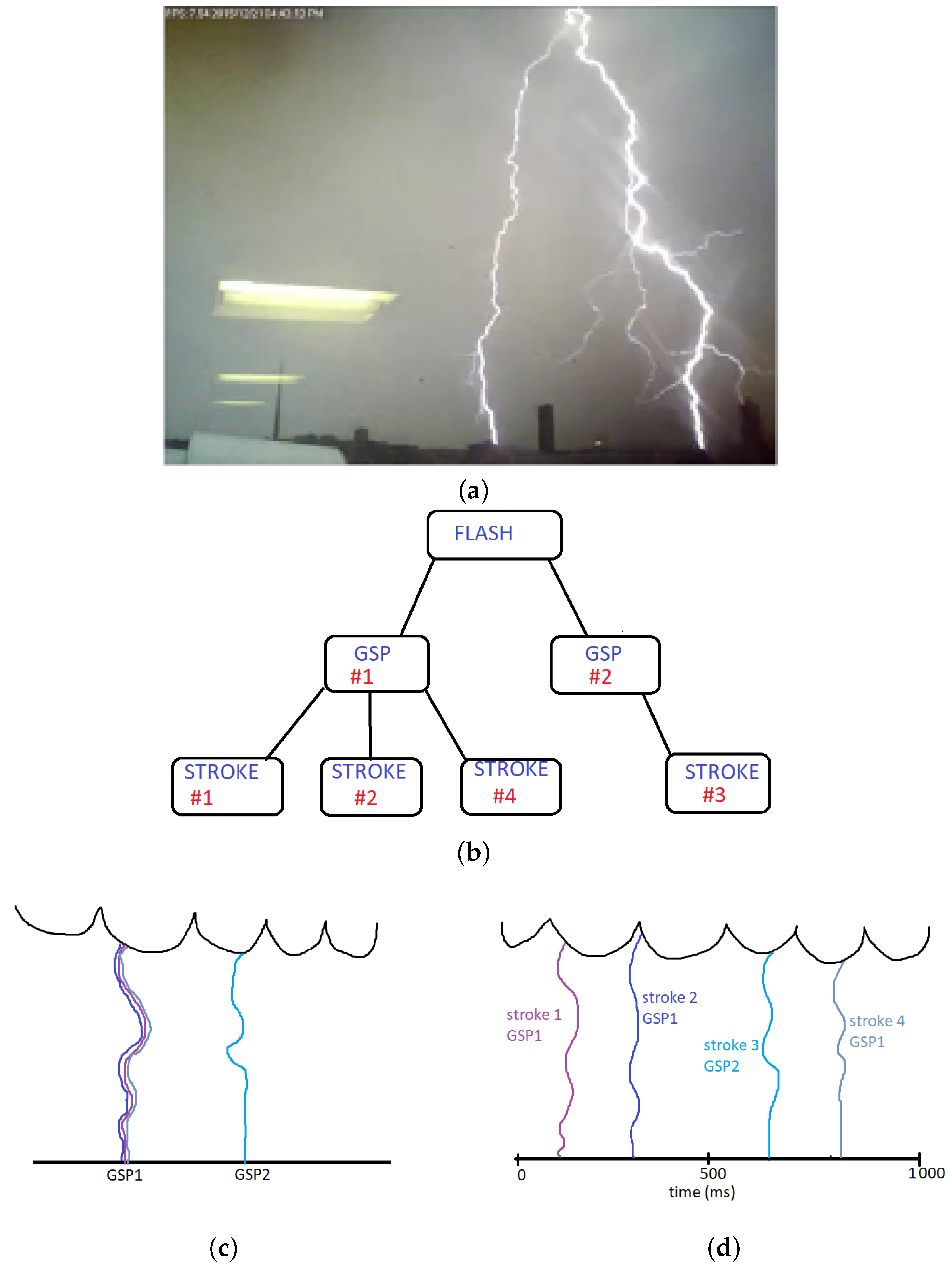
Number of detectors (num_dfrs)	The number of detectors that captured a particular lightning stroke.

. An additional feature, flash number, was used to categorize the lightning strokes according to IEC 62585 [1]. Strokes with an inter-stroke delay of 500 milliseconds and a maximum distance of 10 km between them were categorized as a single flash. The ground truth dataset is represented by the feature strike point, which was validated using high-speed cameras capturing events to the millisecond.

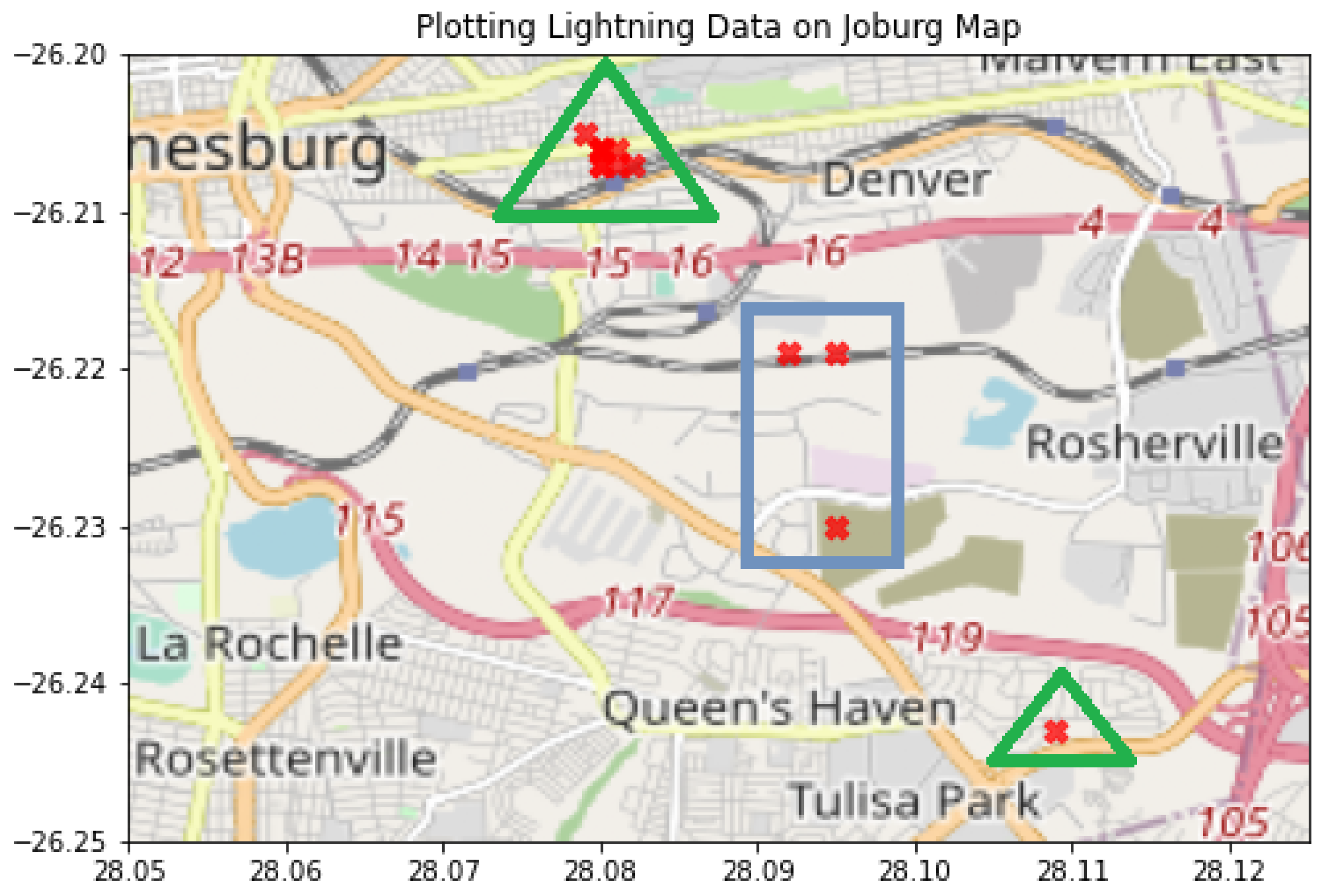
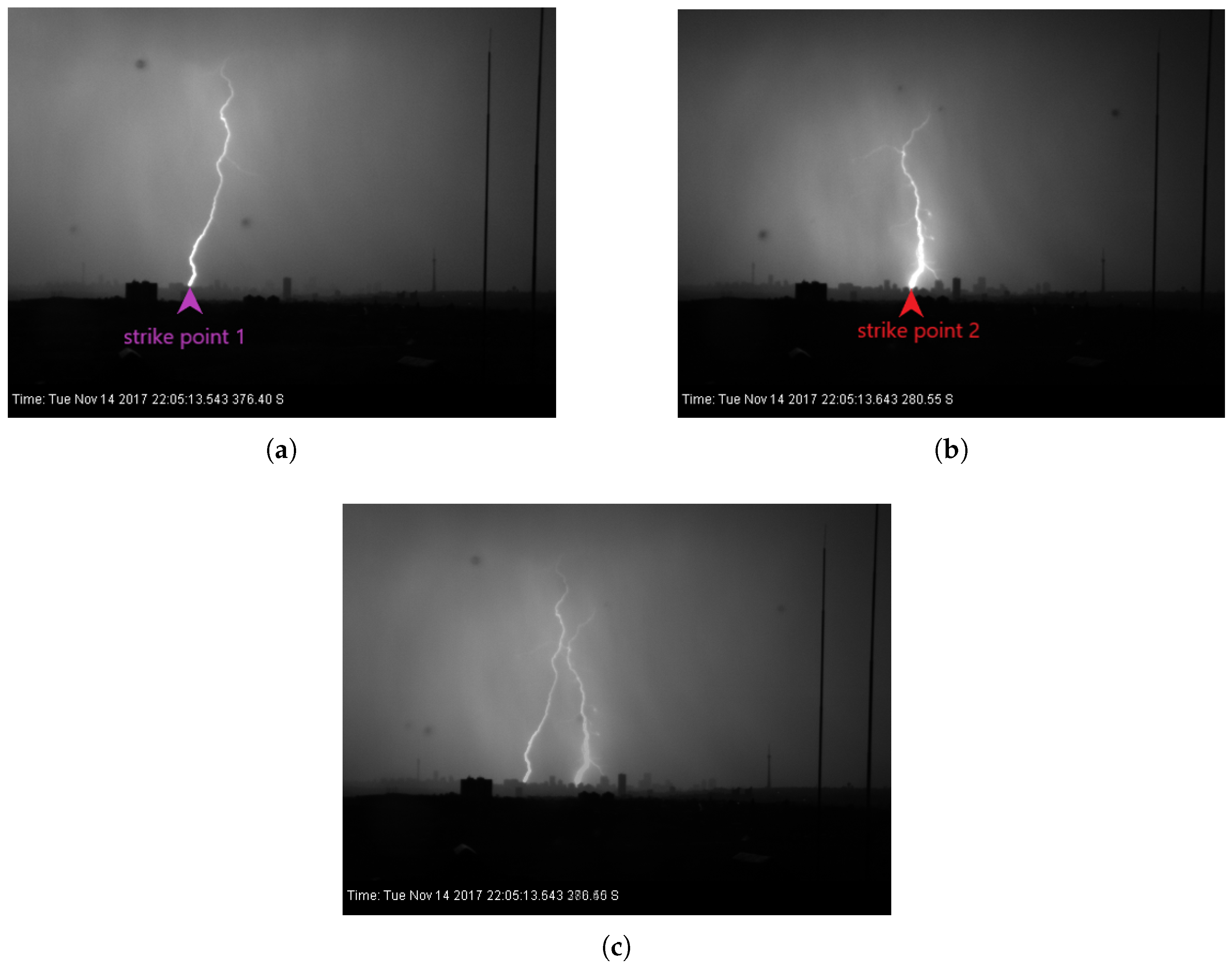
Figure 3 shows an image representation of lightning flash 74 from the data over a map of Johannesburg. The red crosses indicate GSP locations of strokes captured by the LLSs. Figure 4 displays images of the two strike points captured by a high-speed camera. The time stamps indicate that the strokes occurred within a tenth of a second apart, confirming they are part of the same flash.

The semi-major and semi-minor distances were converted from kilometers to degrees for consistency. Time was converted from hours:minutes:seconds to seconds to be read as a float. The dataset has 463 flashes, with 213 single-stroke flashes excluded as they do not have a PSP variable.

3.3. Methods

The aim of this analysis was to determine the GSP of a stroke given the GSP of the previous stroke for flashes that have more than one stroke. To make such predictions, another feature was added: the previous strike point (PSP). First, the data were categorized according to the flashes, then single-stroke flashes were removed as they were not significant for the purpose of the project. The stroke labels in each flash were observed and were used to determine the value of the PSP. If a stroke label is the same as the previous one, PEC, then the PSP label for that entry is 1; if it is not the same, NGC, then the PSP label is 0. The data have more strike points classified as NGCs than PECs: this is in alignment with the observation made in the research of global GSP characteristics in negative downward flashes [12], which then creates a class imbalance. It should also be noted that the initial stroke of each flash was removed since it does not have a PSP value.

BN-learn is an R package that is capable of Bayesian network modeling analysis by means of structure learning, parameter learning, and inference [41]. The package contains algorithms for data pre-processing, inference, parameter learning, and structure learning that combines the data and prior knowledge [41] that are necessary for Bayesian network modeling. It is capable of handling discrete Bayesian networks, Gaussian Bayesian networks, and conditional linear Gaussian Bayesian networks using real data [41].

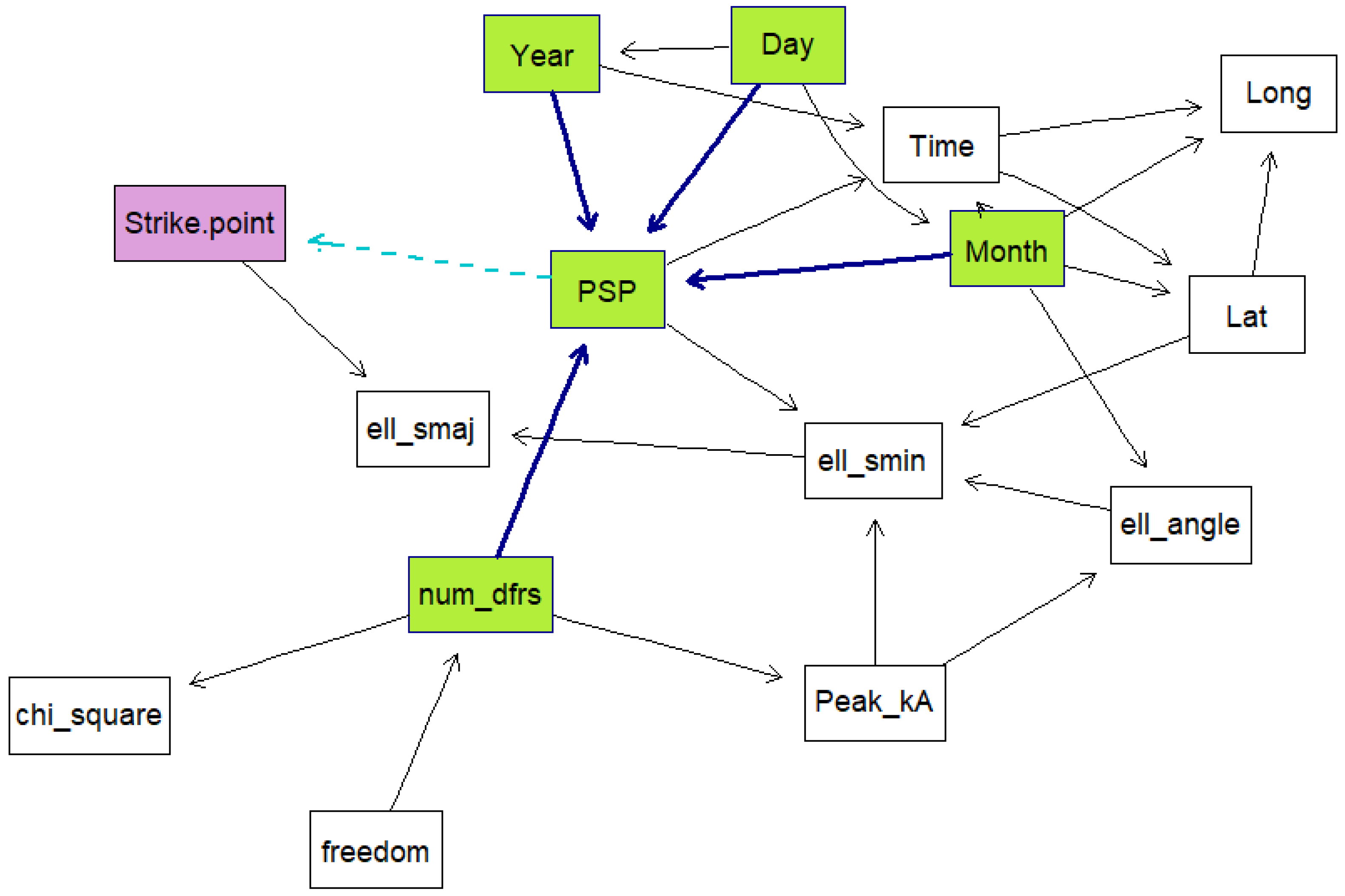
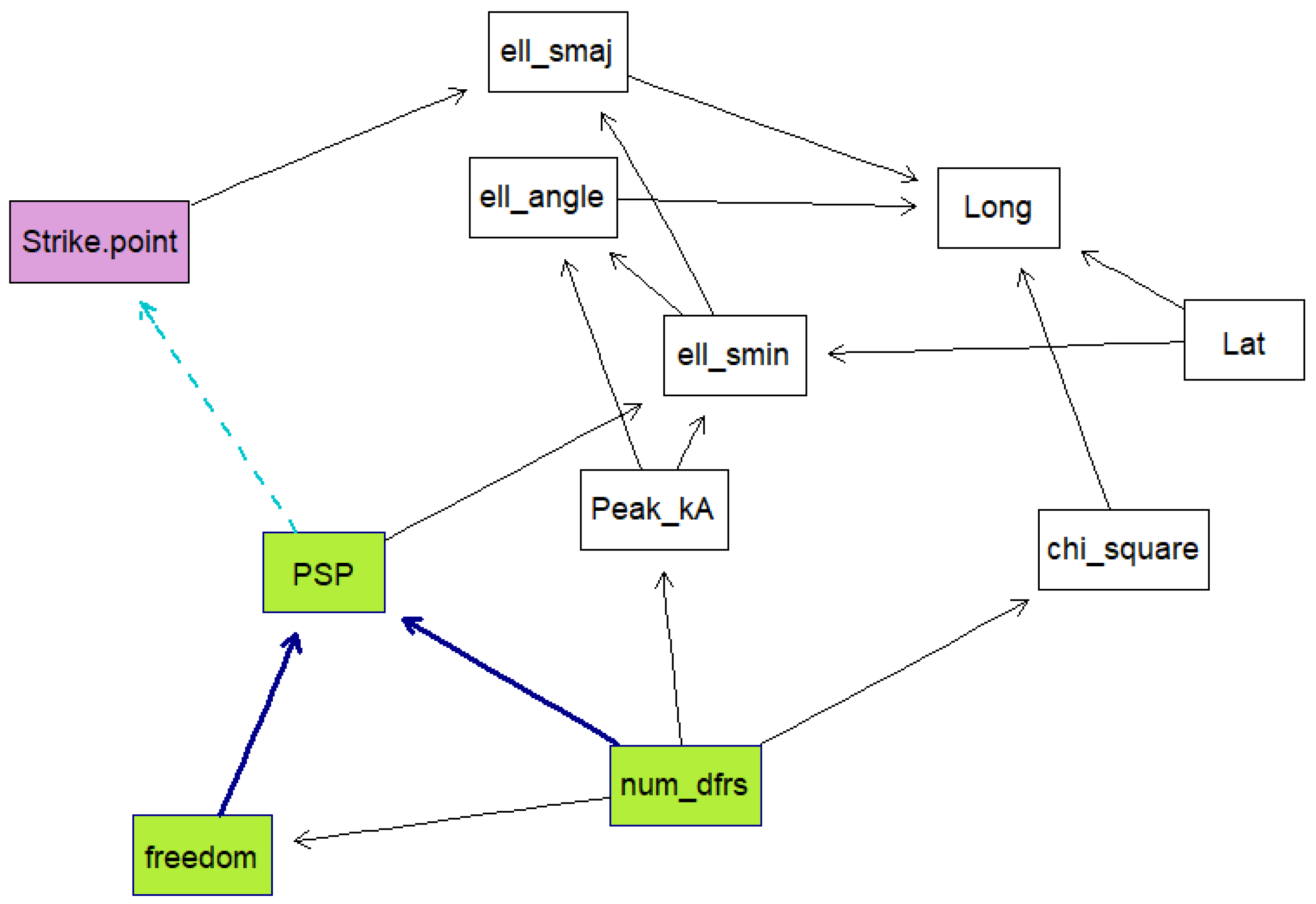
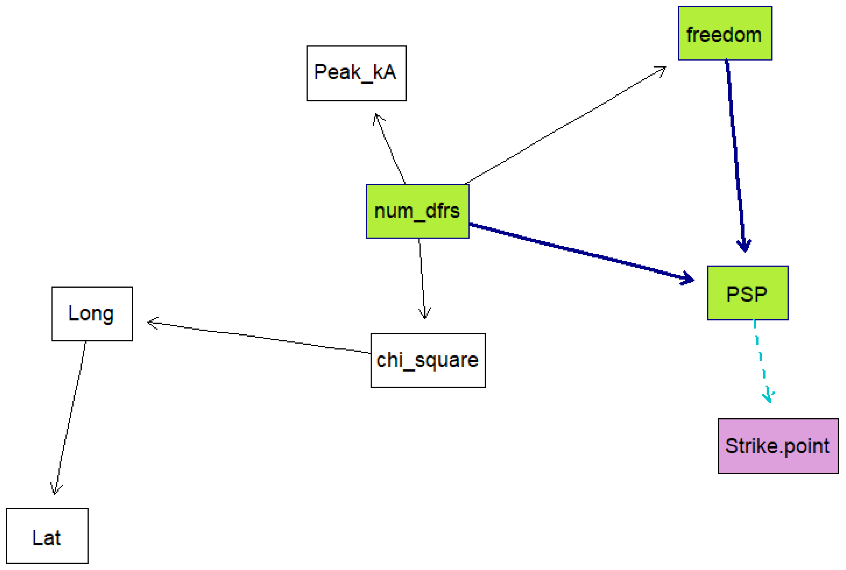
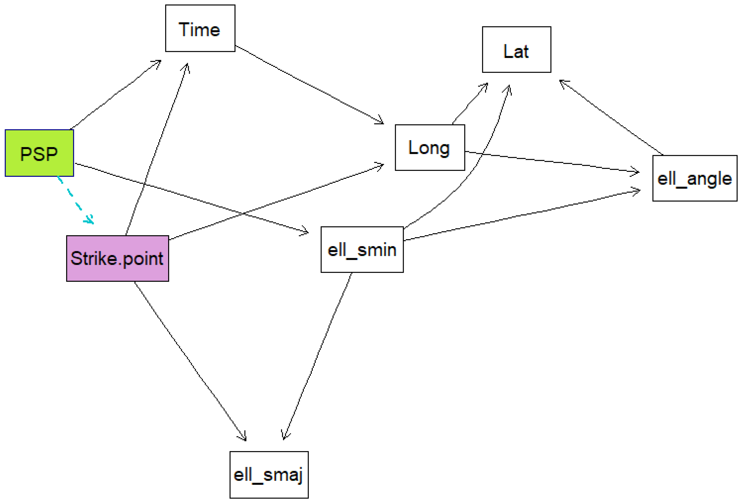
Five Bayesian network models were created using the data. For each model, a k-fold cross validation was run 50 times on the data to obtain the mean classification errors and their standard deviations. This is done to evaluate how well the models are expected to perform. K-fold cross validation is a training method whereby the training data are divided into $k=10$ samples, then $k-1$ samples are trained while the other sample is used as the testing sample. The algorithm is repeated until all the samples have been used as the testing sample, then the average loss is calculated as the performance measure. The models were trained using a score-based structure-learning procedure with tabu search. The first model included all the variables and was trained from the raw data. The second model was trained with all the variables and with the date information set as the conditional dependencies of PSP. The third model excluded dates and times, while the fourth model excluded dates, times, and ellipse information. Both these models had the number of sensors and the degrees of freedom set as parent nodes of PSP. The last model was created using the time, strike point, PSP, latitude and longitude and ellipse information.

The algorithm used for creating the models involved a structure-learning procedure with tabu search and the Bayesian information criterion (BIC). The full code is available on GitHub: https://github.com/Lwano31/BN_models (accessed on 11 May 2024) [40,42]. The steps of the algorithm are summarized as follows:

• Set up conditional dependencies from the data.
• Learn the best-fit directed acyclic graph (DAG) from data with dependencies.
• Perform cross validation on the DAG (data = DAG, runs = 50).
• Calculate the loss with target = PSP.
• Predict the output from the fitted DAG.
• Plot the DAG.
• Repeat the algorithm for the other models.

This is captured in the following code sample:

• net = tabu(flash_data, score = ‘bic-g’)
• graphviz.plot(net, shape = ‘rectangle’,
• layout = ‘fdp’, highlight =
• list(nodes = c (“PSP”, parents(net, “PSP”)),
• arcs = incoming.arcs(net, ”PSP”),
• col = “darkblue”, fill = "tomato", lwd = 3))
•  
• bn.cv(data=flash_data, net, runs=50
• loss.args = list (target = ‘PSP’))
•  
• predicted = predict(bn.fit(net, flash_data), “PSP”, flash_data)

3.4. Analysis

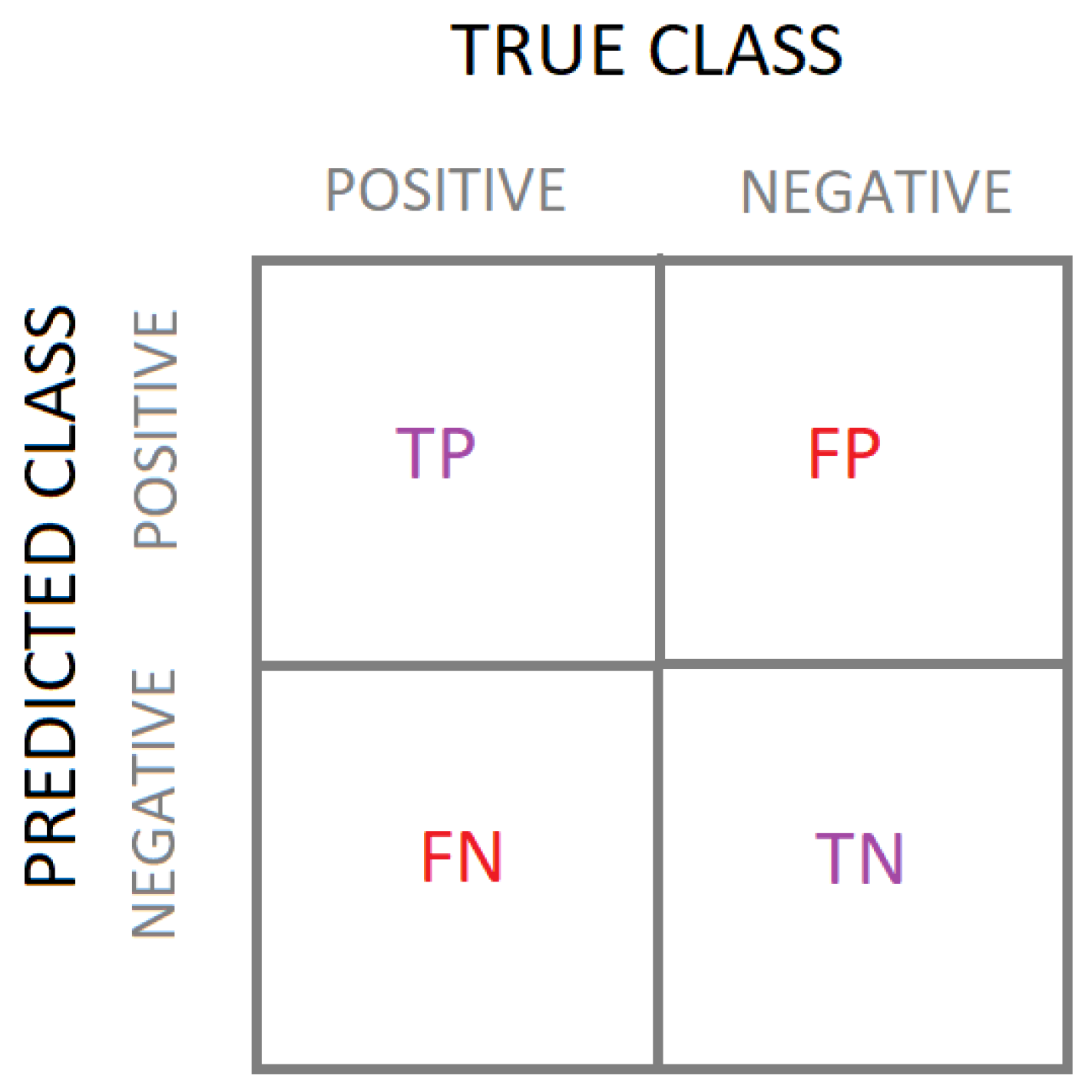
The performance of the models was evaluated using a confusion matrix, which is suitable for binary classification models [43]. Figure 5 shows a schematic of a confusion matrix with the true and predicted class values. It computes the ratio of true positives (TPs), false positives (FPs), true negatives (TNs), and false negatives (FNs), allowing the calculation of performance measures such as accuracy, precision, recall, and F1-score.

$$\begin{array}{cc}\hfill Precision& =\frac{TP}{TP+FP},\hfill \end{array}$$

(10)

$$\begin{array}{cc}\hfill Recall& =\frac{TP}{TP+FN},\hfill \end{array}$$

(11)

$$\begin{array}{cc}\hfill F1-score& =\frac{2\times \mathrm{Precision}\times \mathrm{Recall}}{\mathrm{Precision}+\mathrm{Recall}},\hfill \end{array}$$

(12)

$$\begin{array}{cc}\hfill Accuracy& =\frac{TP+TN}{TP+TN+FP+FN}.\hfill \end{array}$$

(13)

Balanced accuracy and kappa statistics were also used to evaluate model performance while taking into account the class imbalance [43,45].

Baselines

The following baseline algorithms were used for comparison:

• Naive Bayes: constructs a Bayesian probabilistic model assuming all variables are independent [46];
• Multilayer perceptron (MLP): a neural network that assigns weights to multiple variables to produce a binary output [47];
• Logistic regression: similar to MLP but uses an activation function like sigmoid to obtain an output [47];
• Random tree: a decision tree generated from random datasets [48];
• Random forest: a combination of tree classifiers with random sampling [49];
• Sequential minimal optimization (SMO): optimizes a support vector machine (SVM) using Lagrangian multipliers [50].

The methods have various limitations due to the tools used and the type of data. The data are a hybrid of discrete and continuous data for which BN-learn has only one loss function that is suitable. BN-learn only has two algorithms for maxima and minima searches. Another limitation of BN-learn is that discrete nodes can only be parent nodes of continuous nodes: even with prior knowledge of a continuous node being a parent of a discrete node, the library does not allow that.

4. Results

4.1. Directed Acyclic Graphs

Figure 6, Figure 7, Figure 8, Figure 9 and Figure 10 are the Bayesian networks produced using a score-based structure-learning procedure on BNlearn with tabu search with a BIC scoring function that is suitable for data that are a hybrid of continuous and discrete data. The green highlighted nodes are the PSP, which are the target value and its parent node, and the edges from the parent nodes to the target node are highlighted in navy blue. In the first model, Figure 6, the probability distribution of PSP has a conditional dependence on the year. The second model, Figure 7, shows that PSP depends on the year, month, day, and number of sensors, and the third Bayesian network model, Figure 8, shows that in these, the probability distribution of PSP has a conditional dependence on the flash number and the number of sensors. The fourth model, Figure 9, shows that on this model, the probability distribution of PSP has a conditional dependence on the flash number and the number of sensors. In the last model, Figure 10, PSP is a parent node and has no dependence on other features.

The first model (Figure 6) included all the variables and was trained from the raw data without conditional dependencies. The probability distribution of PSP shows conditional dependence on the year. The descendant node of PSP is the semi-minor axis of the uncertainty ellipse.

The second model (Figure 7) included all the variables from the LLS data, but now, conditional dependencies were set for PSP. The model shows that PSP depends on the year, month, day, and number of sensors. The descendant node of PSP is the semi-minor axis of the uncertainty ellipse.

The third model (Figure 8) then excluded the year, month, day, and time features. The parent nodes of PSP are the number of sensors and degrees of freedom. The descendant node of PSP is the semi-minor axis of the uncertainty ellipse.

The fourth model (Figure 9) was then trained with selected LLS variables: latitude, longitude, peak current, chi-square, degrees of freedom, and number of sensors. The target value, PSP, has conditional dependencies on the degrees of freedom and number of sensors.

Finally, the fifth model (Figure 10) was trained with the time, longitude, latitude, semi-major and semi-minor axes of the uncertainty ellipse, and the ellipse angle. The target value, PSP, is a parent node with no conditional dependence on other features. The descendants of PSP are the time, longitude, and semi-major axis of the uncertainty ellipse.

4.2. Performance Measures

The comparative performances of the models, as summarized in

Table 3. Overall model performances with accuracy, balanced accuracy, and kappa statistic.

Model	Accuracy	Balanced Accuracy	Kappa
Model 1	86.7%	73.6%	0.53
Model 2	93.9%	88.0%	0.76
Model 3	90.5%	81.8%	0.64
Model 4	90.8%	81.1%	0.65
Model 5	88.8%	77.3%	0.57

, reveal notable differences in accuracy, balanced accuracy, and kappa statistics. Model 2 stands out with the highest accuracy (93.9%), balanced accuracy (88.0%), and kappa statistic (0.76), indicating superior overall performance. This suggests that the specific features or algorithms used in Model 2 are more effective for this application compared to the others. In contrast, Model 1, while satisfactory, shows the lowest performance metrics in each category, which may signal potential areas for improvement, such as parameter tuning or feature selection. Models 3 and 4 demonstrate moderately high performance, with Model 4 slightly leading in accuracy but trailing in balanced accuracy compared to Model 3. Model 5, with performance metrics generally in the mid-range, offers a balance but highlights room for enhancement in balancing classification accuracy across different classes.

Table 4. Predictive performance of target values for each model with precision, recall, and F1-scores.

Model	Precision	Recall	F1-Score
Model 1 NGC	70.0%	51.5%	59.3%
Model 1 PEC	91.2%	95.8%	93.4%
Model 2 NGC	81.8%	79.4%	80.6%
Model 2 PEC	96.1%	96.6%	96.4%
Model 3 NGC	70.7%	69.1%	69.9%
Model 3 PEC	94.1%	94.5%	94.3%
Model 4 NGC	73.4%	66.9%	70.0%
Model 4 PEC	93.8%	95.4%	94.6%
Model 5 NGC	66.7%	60.3%	63.3%
Model 5 PEC	92.6%	94.2%	93.4%

details the predictive performance of the five models, highlighting their precision, recall, and F1-scores across two categories: new ground channel (NGC) and pre-existing channel (PEC). Notably, Model 2 exhibits superior performance, with precision scores exceeding 80% for NGC and reaching 96.1% for PEC and closely mirrored by its recall and F1-scores. Conversely, Model 1, while effective for PEC predictions, shows room for improvement in NGC detection, indicating potential areas for model refinement. The detailed performance metrics, particularly the F1-scores, underscore the varying strengths of each model at balancing precision and recall, which are essential for optimizing GSP classification.

Figure 11 shows the box plots of the classification errors for the k-fold cross validation of the five BN models over 50 runs. The classification errors for each model are summarized in

Table 5. K-fold cross validation results with mean classification errors and their standard deviations.

Model	Mean Classification Error	Standard Deviation
Model 1	0.1174	0.0042
Model 2	0.1494	0.0051
Model 3	0.1294	0.0045
Model 4	0.1293	0.0046
Model 5	0.1248	0.0032

, which indicates the mean classification errors and standard deviations for a k value of 10 and 50 runs.

The classification errors of the models vary, with Model 1 having errors between 0.108 and 0.126, Model 2 having errors between 0.138 and 0.159, Model 3 having errors between 0.122 and 0.151, Model 4 having errors between 0.119 and 0.140, and Model 5 having errors between 0.118 and 0.132.

5. Discussion

Model 1 (Figure 6) was trained using all variables and shows PSP dependence only on the year. It produced the lowest accuracy and kappa index, indicating that the year alone is insufficient. The model had the lowest mean classification error during k-fold cross validation, suggesting a narrow error range but limited predictive capability. Model 2 (Figure 7) included date information and the number of sensors as conditional dependencies. It achieved the highest accuracy (93.9%) and kappa statistic (0.76), despite having the highest mean classification error. The classification error was evenly spread around the mean, suggesting higher uncertainty due to outliers. Model 3 (Figure 8) excluded date and time features and showed PSP dependence on the degrees of freedom and number of sensors. It produced the third-highest accuracy and kappa statistic, indicating reduced performance without time and date information. The classification error distribution suggested higher mean error uncertainty. Model 4 (Figure 9) excluded date, time, and ellipse information. It performed slightly better than Model 3, implying that ellipse information does not significantly affect PSP prediction. The classification error was similar to that of Model 3, with high mean error uncertainty. Model 5 (Figure 10) used only the ellipse information and time, with PSP as a parent node. It produced the lowest accuracy and kappa statistic but had a narrow error range, indicating consistent but limited performance.

Overall, Model 2 outperformed the others, showing that BNs benefit from set conditional dependencies. Class imbalance slightly affected all models, with lower precision, recall, and F1-scores for NGC strokes compared to PEC strokes. High kappa statistics indicated substantial agreement between actual and predicted targets.

5.1. Baseline Discussion

Other machine learning algorithms were trained on the data, and k-fold cross validation was performed; the results are compared to those of the BN (

Table 6. Predictive performance of target value using other machine learning algorithms as baselines, with precision, recall, and F1-scores.

Classifier	Precision	Recall	F1-Score
Bayesian Network NGC	81.8%	79.4%	80.6%
Bayesian Network PEC	96.1%	96.6%	96.4%
Naive Bayes NGC	61.6%	56.6%	59.0%
Naive Bayes PEC	91.8%	93.3%	92.5%
Logistic NGC	54.1%	44.1%	48.6%
Logistic PEC	89.7%	92.8%	91.2%
ML Perceptron NGC	58.6%	47.8%	52.6%
ML Perceptron PEC	90.4%	93.5%	91.9%
Random Forest NGC	50.8%	22.8%	31.5%
Random Forest PEC	86.7%	95.8%	91.0%
Random Tree NGC	43.0%	40.4%	41.7%
Random Tree PEC	88.8%	89.7%	89.2%
SMO NGC	61.6%	56.6%	59.0%
SMO PEC	91.8%	93.3%	92.5%

and

Table 7. Overall model performances using other machine learning algorithms as baselines, with accuracy and kappa statistic.

Classifier	Accuracy	Kappa
Bayesian Network	93.9%	0.76
Naive Bayes	87.4%	0.52
Logistic Regression	85.0%	0.40
ML Perceptron	86.2%	0.45
Random Forest	84.1%	0.24
Random Tree	81.8%	0.31
SMO	87.4%	0.52

). The BN produced better predictive performance than all the other algorithms, especially for NGC strokes, indicating better handling of the class imbalance. Naive Bayes and SMO were the second-best performers, while random tree had the poorest results.

5.2. K-Means and BN Discussion

When comparing BN models with k-means algorithms (

Table 8. Summarized results from global GSP characteristics in negative downward lightning flash research [13] using three algorithms used in the current literature combined with the results from BN models.

Algorithm	NGC (%)	PEC (%)	All Strokes (%)
Meteorage K-means	63.8–92.0	84.4–99.4	79.9–90.6
GroupGCP	64.6–95.3	87.6–99.4	80.3–94.4
Matsui K-means	98.3–99.1	63.8–79.3	83.1–89.7
Bayesian Network	66.7–73.4	91.2–96.1	86.7–93.9

), BN models fall within the performance range of all three k-means algorithms, particularly for identifying PEC strokes. However, k-means algorithms outperformed BN models at identifying NGC strokes. GroupGCP had the best overall performance, while BN models demonstrated substantial agreement between actual and predicted targets. K-means algorithms rely on predetermined distance thresholds and other conditions, making them easy to implement with high accuracy. BN models, however, provide an algorithm that does not rely on predetermined parameters and offers insight into data feature dependencies.

This comparison makes for a clear answer to the question of whether a Bayesian network approach is relevant for the classification of GSPs. Quite simply, the answer is ‘no’. While the Bayesian network approach does not require an artificial distance threshold to be implemented—and can possibly identify other dependencies other algorithms do not rely on—this does not yield any measurable performance increase. On top of that, it is a significantly more complex approach to implement. As such, it is recommended that the established k-means approaches continue to be used.

5.3. Future Work

This analysis can be improved by using a distance threshold to determine the target value, as used in the k-means algorithms. Even though k-fold cross validation works well for imbalanced data, the problem could be alleviated by applying a SMOTE technique during the pre-processing of data to make the minor class have the same number of samples as the major class. Making use of other programming tools and libraries with Bayesian network capabilities could be an interesting investigation, particularly to compare the results with the ones obtained in this research. Another investigation that could be done in the future would be to use the obtained DAGs from the BN models to learn the parameters of other lightning data from various LLSs, such as the data used for global GSP characteristics in negative downward lightning flashes research from Brazil, Austria, France, Spain, and the United States of America [13].

6. Conclusions

The purpose of this research was to investigate whether Bayesian networks (BNs) offer a viable solution to ground-strike point (GSP) classification based on locations obtained by lightning locating systems (LLSs). Bayesian networks, as probabilistic directed acyclic graphs, learn the joint probability distribution of variables from a dataset, which can then be used to predict GSPs for each lightning stroke. The objectives were to obtain lightning data, select relevant features, categorize the dataset into lightning flashes according to IEC 62858, develop BN models, and analyze the models’ performance. These objectives were successfully achieved using lightning data provided by the South African Weather Service. The BN models were developed through a structure-learning procedure and analyzed using confusion matrices and kappa statistics.

Five BN models were created using various combinations of variables. The first model used raw data, while subsequent models incorporated assumptions about joint probabilities. Although the first model had the lowest mean classification error during cross validation, the second model produced the best results, with an accuracy of 93.9% and a kappa index of 0.73. Six algorithms—Naive Bayes, logistic regression, multi-layer perceptron, random tree, random forest, and sequential minimal optimization—were used as baselines. While all produced good results, BN outperformed them. Both BN and the baseline models were affected by class imbalance, with the minor class having worse prediction results.

When comparing BN models to the k-means algorithms used in global GSP characteristics research [13], k-means performed better overall. The highest accuracy of BN models was slightly lower than GroupGCP but higher than Meteorage and Matsui k-means. Despite BN’s good performance, k-means remains the best method for GSP analyses due to its ease of implementation and consistent results. In summary, while Bayesian networks offer an alternative for GSP analysis, they do not surpass the performance of k-means methods. However, BN models provide valuable insights and handle class imbalances effectively, making them a viable complementary approach to existing methods.