1. Introduction
The transition to renewable energy sources is being increasingly acknowledged as a critical strategy for mitigating air pollution and combating global warming [
1,
2]. Offshore wind energy, which is enabled by advances in floating turbine technologies, presents a sustainable solution for reducing our reliance on fossil fuels, significantly contributing to CO
2 emissions and climate change [
3]. Renewable energies, such as wind power, play a pivotal role in decarbonizing the energy-production sector and mitigating the environmental and health impacts of air pollution. Diseases linked to air pollution, such as chronic respiratory conditions, cardiovascular diseases, and lung cancer, pose substantial public health challenges, underscoring the pressing need for cleaner energy alternatives [
4,
5]. Moreover, incorporating renewable energies into the electricity sector can yield positive social, environmental, and economic outcomes, aligning with global initiatives to achieve a sustainable and low-carbon future [
6].
Floating offshore wind turbines (FOWTs) mark a significant advancement in harnessing wind energy, providing access to deeper waters where winds are consistently stronger. Unlike their fixed-bottom counterparts, FOWTs can be deployed in deep waters, thus exploiting vast untapped wind energy potential far from the shore. This adaptability reduces visual impact and navigational risks while maximizing energy capture [
7]. The importance of accurately forecasting metocean data, such as wind speed and significant wave height, cannot be overstated in the context of FOWTs. These forecasts are crucial for offshore wind farm development’s design, operation, and maintenance phases. Precise metocean forecasts facilitate optimal turbine placement, enhancing energy production and efficiency [
8,
9]. They also improve safety and reduce operational costs by identifying ideal timeframes for installation and maintenance tasks, thus minimizing downtime and extending the lifespan of wind farms [
10,
11]. Moreover, incorporating metocean data into the planning and operational frameworks of offshore wind farms plays a vital role in enhancing the reliability and stability of the power grid. This integration aids in mitigating environmental impacts by ensuring that the dynamic marine environment is considered in FOWT designs, safeguarding marine ecosystems, and fostering sustainable development [
12]. Integrating renewable energy sources into the power grid requires advanced forecasting techniques to handle the inherent variability and uncertainty of natural resources like wind and ocean waves. Recent advancements in machine learning (ML) have demonstrated promising results in forecasting wind speed and wave height, which are essential factors for optimizing the performance of renewable energy systems [
13]. This literature review explores various ML approaches used to predict wind speed and wave height, highlighting their contribution to enhancing renewable energy integration and efficiency.
ML algorithms, such as support vector machines and random forest models, have been used to develop predictive models for runoff, demonstrating their effectiveness in forecasting and highlighting their potential in environmental applications [
14]. A recent study explored using machine learning (ML) methods to forecast offshore wind speed, wave height, and alignment to optimize the operational performance of floating offshore wind turbines [
15]. Through the application of nonlinear autoregressive with exogenous input (NARX) neural networks and Gaussian process regression (GPR), their study demonstrates the capability of ML to improve the precision of metocean predictions. This advancement contributes significantly to the efficiency and safety of renewable energy sources within marine settings. Another study presented an innovative approach to forecasting chaotic and random wind speed patterns by combining the Volterra series with machine learning (ML) techniques [
16]. This study focuses on predicting Volterra kernels up to the third order, employing a forward–backward propagation neural network trained on 12-month wind speed data from the Fujairah site in the United Arab Emirates. Their methodology demonstrates the potential of ML in accurately forecasting wind speeds with complex patterns, offering valuable insights for wind energy management and planning. A different study introduced a hybrid machine learning (ML) framework designed specifically for short-term wind speed and power forecasting within smart city power grids [
17]. Their model, which is called EMD-KM-SXL, integrates empirical mode decomposition, K-means clustering, and various ML techniques such as support vector regressor, XGBoost regressor, and Lasso regressor to predict wind speed. The demonstrated performance of this model highlights the effectiveness of ML in improving the accuracy of wind power forecasting, which is vital for the efficient scheduling of smart power generation.
Another study explored the application of Artificial Neural Network (ANN) models for wind speed forecasting at different potential locations in Pakistan [
18]. By analyzing wind speed data at four distinct heights across 12 stations, the researchers demonstrated the capability of ANN models in capturing the variability of wind speeds, which is essential for assessing the wind energy potential of a region. An ultra-short-term forecasting approach for wind speed using lightweight features and ML models was examined in another study [
19]. Their two-step method employs support vector regressor, random forests, and multi-layer perceptron models, indicating the superiority of ML models in predicting wind speed accurately over short intervals. Their study contributes to developing efficient wind energy management strategies by providing reliable wind-speed forecasts. Another study investigated the potential of ML techniques for forecasting wave height over the Ocean of Things, focusing on its relevance to ocean renewable energy generation [
20]. Their study highlights the adaptability of ML methods in predicting oceanic conditions, facilitating the exploitation of wave energy as a renewable resource. A novel hybrid framework that enhances the accuracy of predicting karst spring discharge using historical data tailored for regions with sparse meteorological data was presented in another study [
21]. This framework leverages LSTM models optimized with advanced algorithms and variable screening techniques like partial correlation and mutual information, improving data input quality. Additionally, it employs time series decomposition methods such as LOESS and empirical mode decomposition to simplify the input data, making the model more effective. This approach outperforms conventional models that are dependent on meteorological inputs and offers a robust solution for water resource management in karst areas. Another study proposed a novel approach to daily runoff prediction by integrating physically based models with a long short-term memory (LSTM) network [
22]. Their research addresses the challenges of the non-stationary and time-varying nature of runoff prediction, leveraging the simulation strength of physical mechanism models and the nonlinear analysis capabilities of LSTM. This combination strategy enhances the accuracy of runoff predictions and offers a comprehensive evaluation metric that considers the characteristics of multiple models, showing substantial improvements in forecasting performance across various watershed characteristics. This innovative methodology promises significant implications for water resource management and reservoir operations. In another example, particle swarm optimization (PSO) is integrated with long short-term memory (LSTM) neural networks to enhance flood forecasting [
23]. This approach systematically optimizes LSTM hyperparameters, significantly improving the accuracy and reliability of rainfall-runoff predictions. This methodology is pivotal for effective flood prevention and advances the capabilities of hydrological models in environmental management and disaster mitigation.
This study utilizes three machine learning methods to analyze metocean data collected from an offshore buoy in the Pacific Ocean, northwest of California, with the aim of developing a comprehensive method for predicting wind and wave patterns at a specific offshore site. The short-term prediction of wind and wave conditions with high accuracy significantly contributes to optimizing wind turbine control systems and their efficiency. Accurate predictions for more extended periods help operators schedule maintenance during times of low activity, which reduces downtime and increases the overall availability of the turbines. This optimized scheduling directly impacts the efficiency and lifespan of turbines by ensuring they operate under ideal conditions and receive maintenance before weather-induced wear and tear can occur.
This study focuses on short-term and mid-range, or sub-seasonal, metocean forecasts. Short-term forecasts, spanning 1–3 days, are known for their high precision and are particularly useful for energy-maximizing control purposes and for predicting ship motions during offshore operations. Short-term forecasts of wind and wave conditions, spanning 1–3 days, are crucial for making decisions during marine operations [
24]. Sub-seasonal forecasts generally cover a period from 10 to 30 days, bridging the gap between conventional weather models and longer-term seasonal predictions, which span one to seven months [
25].
Medium-term forecasts are crucial for planning maintenance operations and selecting operational modes for marine renewable energy devices, such as power production or survivability mode [
26]. These forecasts enable offshore engineers to schedule construction, maintenance, and drilling activities during favorable weather conditions, minimizing downtime and enhancing operational efficiency. Accurate forecasts facilitate the optimal allocation of resources, such as deploying vessels and personnel at the right time, thereby reducing costs associated with delays and standbys. Marine operations exceeding 72 h are typically planned as weather-unrestricted, with environmental conditions estimated using long-term statistics that may vary seasonally. Improved weather forecasts, especially for significant wave height and wind speed, can extend the feasible duration of weather-restricted operations [
27]
For wind energy, maintaining turbines involves tasks like working in the nacelle or using cranes, where wind speed safety limits must be observed, meaning work can only proceed when wind speeds are low. These maintenance activities often necessitate hiring cranes, contractors, and other equipment that needs to be booked well in advance, often with a wait time of several weeks [
28]. Knowing expected weather conditions allows for better scheduling by allowing researchers to make decisions further in advance or providing more information than simply relying on average conditions for the season. For instance, knowing if a particular week is forecasted to be more or less windy than usual can help researchers plan the number of jobs to schedule for that week. Extended periods of unusually low wind, sometimes coupled with high demand due to cold weather, can complicate and increase the cost of power system management. Subseasonal-to-seasonal forecasts can offer early warnings about these unusual conditions, allowing for timely preparations and corrective actions [
25].
Although the main focus of this study is on FOWTs, the implications of this research extend beyond the interest of offshore wind. The precise seasonal and sub-seasonal predictions of wind and waves will offer advantages in terms of coastal land management, marine vessel routing, renewable energy sectors, and oil and gas operations [
29,
30,
31,
32].
Even though short-term forecasts are crucial for shaping societal decisions, many important choices must be made several weeks or months before favorable or disruptive environmental conditions occur. For instance, relocating emergency and disaster relief supplies can take weeks or months. However, pre-staging these resources in areas likely to experience extreme weather or disease outbreaks could save lives and maximize the effectiveness of limited resources [
33]. Likewise, emergency managers dealing with unexpected events such as nuclear power plant accidents or large oil spills must communicate the impacts of these events over extended timeframes. Additionally, naval and commercial shipping planners set shipping routes weeks in advance to strategically position assets, avoid hazards, and capitalize on favorable conditions [
33].
Large waves can prevent ships from mooring with oil and gas platforms. Typically, wave heights up to 2 m are within standard operating conditions, while heights between 2 and 3.5 m make docking more difficult. An analysis of North Sea data revealed that over
of wave heights were above 3.5 m in nearly half of the winters studied, leading to difficult mooring conditions. Furthermore, in
of the winters, wave heights of 5 m or more were observed over
of the time, likely compromising platform operability. Thus, wave height forecasts weeks in advance would greatly aid in planning operations that involve oil and gas platforms [
34].
The remainder of this paper is organized as follows.
Section 2 details the machine learning models used in this study, including Facebook Prophet, SARIMAX, and long short-term memory (LSTM), and describes the data acquisition and preprocessing processes. In
Section 3, the performance of these models is evaluated in forecasting wind speed and significant wave height, offering a critical analysis of their effectiveness and practical implications. In
Section 4, findings are synthesized, their significance for offshore wind turbine applications is discussed, and potential avenues for future research are outlined.
2. Methodology
The present study uses three machine learning models—Facebook Prophet, SARIMAX, and LSTM—to predict wind speed and wave height using high- and low-resolution datasets for 1-, 3-, and 30-day periods. The subsequent sections elaborate extensively on these three ML models.
2.1. Facebook Prophet
Facebook Prophet is a prediction tool that manages time series data characterized by trends and seasonality patterns. It is a perfect model for handling irregular data, which are common in business forecasts, often containing missing values or significant outliers, and it typically necessitates minimal data preprocessing [
35]. The objective of the Prophet model is to streamline the forecasting process by automating a substantial portion of the statistical modeling procedure [
36]. In the core of the Prophet model, a decomposable time series model comprising three primary elements of trend, seasonality, and holidays lies represented as follows:
where
is the predicted value;
represents the trend function, which models non-periodic changes;
represents the seasonality or modeling periodic changes,
represents the effects of holidays or events; and
represents the error term accounting for any idiosyncratic changes not accommodated by the model. A detailed analysis of the components of the Prophet model, an exploration of its functionality, and the underlying mechanisms that drive its operations are provided here.
The trend component, denoted as
, is modeled, and a piecewise linear or logistic growth curve is employed to adapt the variations in the time series trend. In the linear model, the trend manifests as a piecewise linear function. Conversely, in the logistic growth model, the trend is influenced by a carrying capacity,
, which is subject to temporal fluctuations and can be expressed as follows:
The seasonality component, denoted as
, is modeled utilizing the Fourier series to accommodate complex seasonal patterns. This feature enables Prophet to capture yearly, weekly, and daily seasonal variations. The Fourier series for seasonality can be represented as follows:
Here,
N is the number of Fourier terms that control the model flexibility,
and
are the Fourier coefficients, and
P is the period. The holidays component
models predictable irregularities on specific dates, like holidays or events, which can be manually specified. It uses an indicator function for each holiday to model its effect as follows:
where
is an indicator function that is 1 if time
t is the
ith holiday and 0 otherwise, and
represents the impact of the
ith holiday on the forecast. Finally, the error term, which is denoted as
, captures any random fluctuations in the data that remain unaccounted for by the model. It is presumed to follow a normal distribution,
, where
represents the variance of the error term.
2.2. SARIMAX
The Seasonal Autoregressive Integrated Moving Average with eXogenous variables (SARIMAX) model is an extension of the Autoregressive Integrated Moving Average (ARIMA) model. The SARIMAX incorporates both seasonality and exogenous variables into the forecasting equation. It is a powerful statistical method used for forecasting time series data that can account for complex patterns, trends, seasonal effects, and the influence of external factors. These features make it capable of capturing complex data patterns beyond trends and noise [
37]. The SARIMAX model can be represented by the notation SARIMAX(p, d, q)(P, D, Q)[s] with exogenous variables, where p stands for the order of the autoregressive (AR) part, d is the degree of differencing, and q denotes the order of the moving average (MA) part. P, Q, and D represent the seasonal components of the AR, differencing, and MA parts, respectively. The exogenous variables represent the external factors that might influence the target variable but are not included in the time series, and s indicates the periodicity of the seasonality. The combined equation for the SARIMAX model is as follows:
This model integrates the effects of autoregression, moving average, differencing, seasonality, and exogenous variables into a single comprehensive forecasting model. The SARIMAX model offers a robust framework for forecasting complex time series data, utilizing internal dynamics and external influences and accounting for seasonality. Internal dynamics are implemented through AR, MA, and differencing, while the external influences are applied via exogenous variables. A breakdown of these key components of the SARIMAX model with insights into its functionality and underlying mechanisms is described here.
The autoregressive term (AR) models the relationship between the current value of the time series data and its past values.
Here, represents the AR polynomial in the backshift operator B, and are the model’s parameters. Finally, applying the backshift operator to results in .
The moving average component (MA) models the error term as a linear combination of past error terms and can be represented as follows:
Similar to AR here, is the MA polynomial in the backshift operator B, and , are the model’s parameters.
Integration component
involves differencing the time series data to achieve stationarity. Here,
d is the order of differentiation. It subtracts the next value by the current value
d times, which helps remove the trends and seasonality in the series.
The seasonal AR and MA components are denoted as and , respectively, where s is the seasonality period and P and Q are the orders of the seasonal AR and MA parts.
Finally, the Exogenous Variables
are external factors that influence the time series data. Here,
represents the coefficients of the exogenous variables and
represents the external factors at time
t.
2.3. Long Short-Term Memory
Long short-term memory (LSTM) models represent a distinct category within Recurrent Neural Networks (RNNs), as they possess the ability to learn long-term dependencies and remember information for long periods within sequential data [
38,
39]. This is a crucial capability in many applications in which the current output is significantly influenced by context and history of information. These models were introduced during training to eliminate the vanishing gradient problem of the traditional RNNs. LSTMs are widely used for sequence prediction problems like natural language processing, speech recognition, and time series forecasting.
The core components of LSTMs typically use special units called cell states equipped with three gates, namely forget, input, and output gates, which regulate the flow of information. The forget gate decides what information should be thrown away or kept and the input gate updates the cell state with new information, while the output gate determines what the next hidden state should be.
Given a sequence of inputs
, an LSTM updates its hidden state
, and cell state
at each time step
t. The forget gate
searches for
and
values and outputs a number between 0 and 1 for each number in the cell state
. Output 1 represents “completely keep”, while 0 represents the action “Eliminate”.
The input gate
decides which values will be updated, and a tanh layer
creates a vector of new candidate values that could be added to the state.
The cell state regulates the forgetting and replacement process of the state with a scale factor for the decision on how the update of each state value should be reflected.
Finally, the hidden state condition
, which contains predictions and information on previous inputs, is decided by the output gate
.
Here, is the input vector at time step t, while and are the hidden and cell states from the previous time step, respectively. W and b determine the weights and biases for the different parts of the system, and the output values between 0 and 1 are achieved using the Sigmoid and hyperbolic tangent functions. When all these components are multiplied elementwise, the state function and the output gate values are obtained.
2.4. Data Acquisition and Preprocessing
The data utilized in this study consist of standard meteorological and descriptive wave measurements obtained from the National Oceanic and Atmospheric Administration (NOAA) in the United States. These measurements were gathered by sensors installed on floating offshore buoys deployed across the United States and international waters, which were managed by the National Data Buoy Center (NDBC). Specifically, data from Station 46059, positioned west of San Francisco, California, was selected for analysis. Situated in the Pacific Ocean off the northwest coast of California (), this offshore buoy provides historical data from October 2015 to April 2021. The dataset contains various measurement parameters, including wind direction (WDIR), wind speed (WSPD), gust (GST), wave height (WVHT), dominant wave period (DPD), average wave period (APD), mean wave direction (MWD), pressure (PRES), air temperature (ATMP), water temperature (WTMP), dew point (DEWP), visibility (VIS), tide (TIDE), and a date column.
The selection of this particular station was motivated by weather stability and sea conditions, which makes it a suitable place for offshore wind turbines without significant disturbances. Moreover, the mean wind speed recorded at this station over the historical data utilized in this study is 8.66 m/s, with a maximum wind speed of 23.36 m/s at the hub height of NRELs (National Renewable Energy laboratories) 5MW offshore wind turbines. These wind speeds fall within the operational range of these wind turbines, further justifying the choice of this station for analysis.
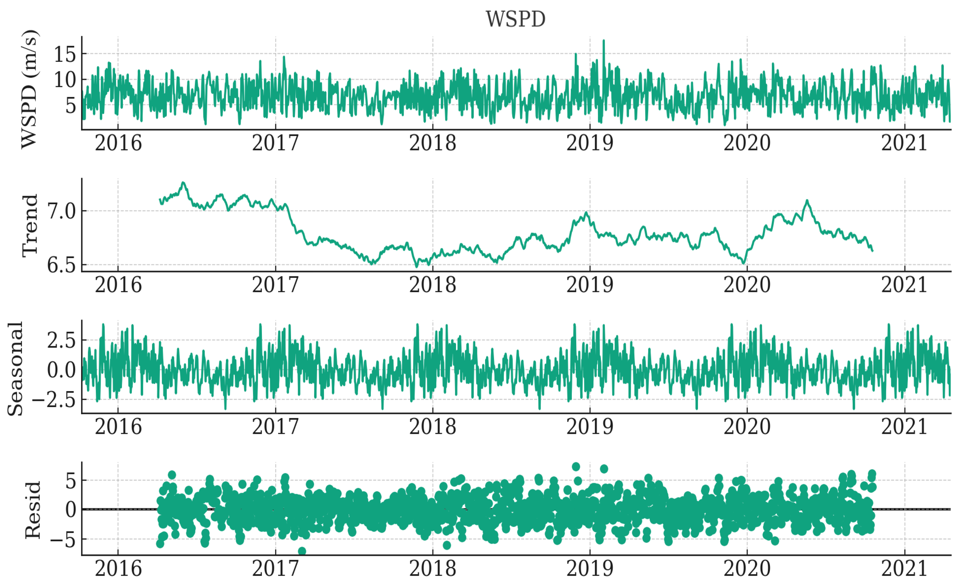
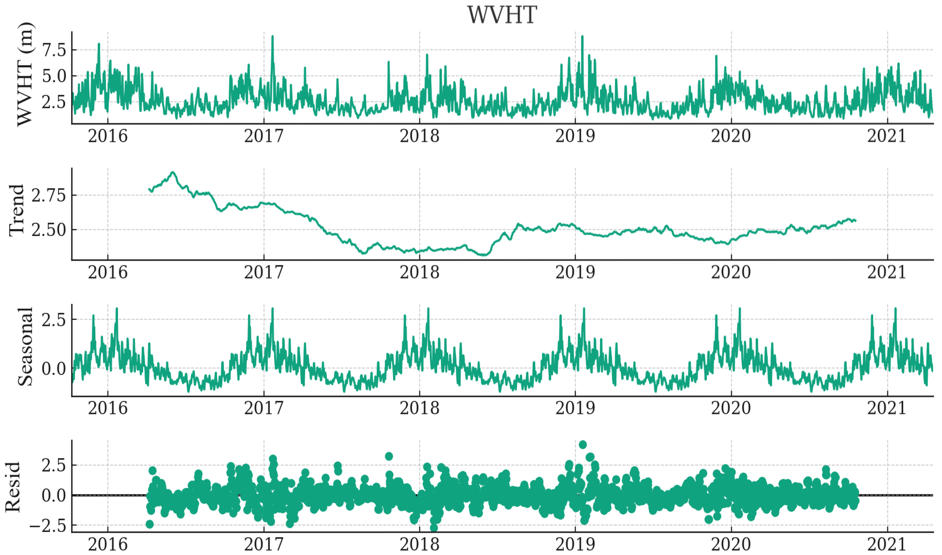
The high-resolution meteorological data files feature a sampling frequency of 10 min for wind speed and one hour for significant wave height. These data were resampled to a daily sampling frequency to create a low-resolution dataset for longer 30-day forecasts. This study focuses on forecasting wind speed and wave height for 1, 3, and 30 days using high- and low-resolution data. The data were resampled to daily frequency using average values, and any missing values were filled out using linear interpolation to prepare for machine learning models. After handling missing values, a seasonal decomposition was performed to gain insights into the seasonality of the data. This decomposition reveals three key components: trend, seasonality, and residual, as demonstrated in
Figure 1 and
Figure 2 for WSPD and WVHT. The analysis indicates the presence of seasonal patterns in the wind speed data, which aligns with expectations given the influence of seasonal weather patterns on wind speed. The Augmented Dickey–Fuller (ADF) test results for wind speed data show a value of
for the test statistic, 0.0 for the
p-value, and the number of lags and observations used are 1 and 2018, respectively. Moreover, the critical values for
,
, and
confidence levels are
,
and
, respectively.
The ADF test statistic is far less than the critical values, and the
p-value is 0.0, indicating strong evidence against the null hypothesis. The null hypothesis can be rejected with confidence, and it can be concluded that the series is stationary. The results of the seasonal decomposition offer valuable insights into the underlying structure of the Wave Height (WVHT) data, as depicted in
Figure 2. While WVHT displays a certain level of predictability through its seasonal patterns, any long-term changes indicated by the trend do not stem from non-stationary processes but signify a stable evolution over time. This analysis underscores the importance of considering seasonal influences and long-term trends when comprehending and forecasting wave height dynamics. Moreover, the absence of significant residuals suggests that the decomposition model effectively captures the primary dynamics of the data. This makes it a potentially valuable tool for further analysis and decision-making related to oceanic and coastal activities.
The ADF test results for WVHT data indicate a value of for the test statistic and for the p-value, and the number of lags and observations used are 14 and 2004, respectively. Moreover, the critical values for , , and confidence levels are , , and , respectively. Like the ADF for WSPD, the null hypothesis with a high confidence level can be rejected, as the ADF of WVHT is significantly lower than the critical values for confidence levels, meaning the WVHT time series is stationary. The p-value for WSPD and WVHT is also very small, supporting the conclusion that the time series is stationary and does not have a unit root. This implies that the mean and variance of the WVHT and WSPD data do not have time-dependent structures that would require differencing to make them stationary.
Choosing a suitable exogenous variable (EXOG) for an ML model depends on the specific context and the hypothesis about what might influence the variables that are being predicted, which in this study are WSPD and WVHT. Exogenous variables are external factors that could have a predictive relationship with the target variable. The following features might be considered as exogenous variables for wind speed forecasting.
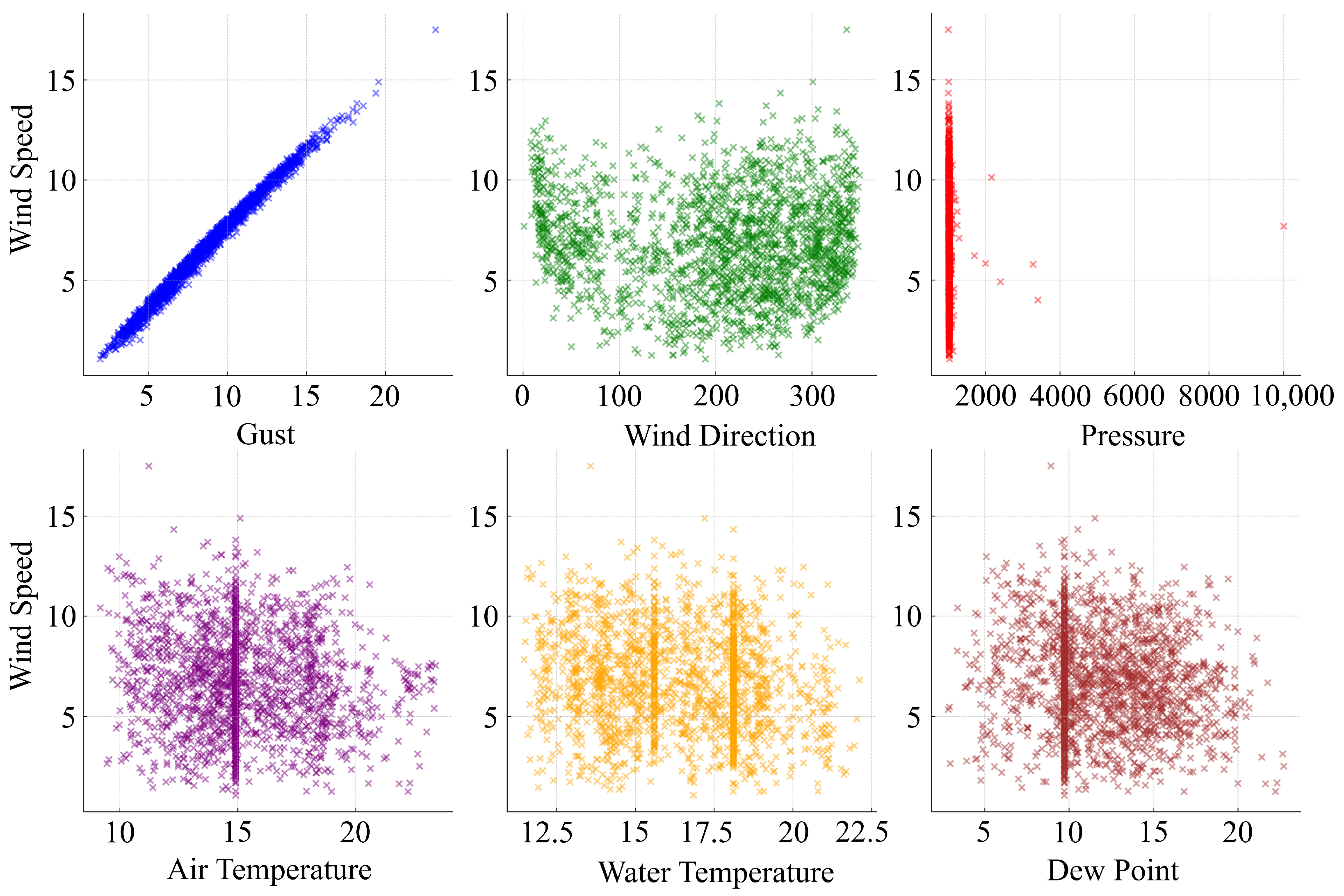
Changes in atmospheric pressure (PRES) can influence wind patterns and speeds. Lower pressure often leads to higher wind speeds as air moves from high- to low-pressure areas. In addition, temperature differences can cause pressure differences, leading to wind. The difference between air temperature (ATMP) and water temperature (WTMP) might also be significant, especially for coastal areas or over bodies of water. Furthermore, the air’s humidity or dew point (DEWP) can affect atmospheric conditions and, consequently, wind patterns. Likewise, the wind direction (WDIR) could affect the context for seasonal wind patterns or shifts that influence speed. To evaluate the connection between potential exogenous variables and wind speed, an exploratory data analysis (EDA) is conducted, concentrating on several selected variables, including PRES, ATMP, WTMP, DEWP, and WDIR. The correlations of these exogenous variables with the wind speed are examined and visualized using scatter plots. This analysis aims to identify variables that exhibit a notable relationship with wind speed, revealing promising candidates for inclusion as exogenous variables in the machine learning models. The correlation coefficients between wind speed (WSPD) and the selected potential exogenous variables, such as atmospheric pressure (PRES) and wind direction (WDIR), indicate a very weak relationship, with negative values of and , respectively. Similarly, the correlation between WSPD and other exogenous variables like air temperature (ATMP), water temperature (WTMP), and dew point (DEWP) also shows a weak relationship, with negative values of , , and , respectively. These correlation values suggest little to no linear relationship between wind speed and the selected exogenous variables. However, it is essential to note that correlation coefficients only capture linear relationships, and there may still be nonlinear or complex interactions between these variables that could impact wind speed. Therefore, further analysis and modeling techniques may be necessary to fully understand the relationship between wind speed and these exogenous variables.
The correlations are relatively weak, with the strongest (yet still weak) negative relationships observed with water temperature (WTMP), air temperature (ATMP), and dew point (DEWP). These negative correlations suggest that as the temperatures and dew point increase, wind speed slightly decreases, possibly due to temperature’s influence on atmospheric pressure and wind patterns. However, the correlations are not strong enough to indicate a direct or significant predictive relationship on their own. Given the weak correlations,
Figure 3 provides a useful visualization of these relationships to look for nonlinear patterns or outliers that might influence the wind speed.
From
Figure 3, it can be concluded that the weak relationships suggest that the considered variables may not be potential exogenous variables in an ML model, as they are not strong predictors of wind speed. Instead, new features that capture a meaningful relationship between air temperature (ATMP) and wind speed (WSPD) were created to be used as exogenous variables in the models. The choice of air temperature is based on the availability of data, domain knowledge, and its correlation with wind speed. While no direct formula universally links air temperature to wind speed due to the complex nature of atmospheric dynamics, a few conceptual ideas that might help generate a new feature that could potentially enhance the model’s ability to predict wind speed can be explored. One concept to consider is the temperature gradient, which measures how temperature changes in space. In meteorology, significant temperature differences can drive wind formation due to pressure differences. Another approach could be creating an interaction term between ATMP and other relevant features, which might unveil hidden relationships. For example, the interaction between ATMP and (PRES) could provide insights, as pressure differences driven by temperature changes are a fundamental cause of wind. In this study, the correlation results between wave height (WVHT) and exogenous variables such as average wave period, gust speed, and wind speed demonstrate relatively higher correlations, with values of 0.643, 0.631, and 0.566, respectively. These findings suggest a stronger linear relationship between wave height and these variables, indicating they may significantly impact wave height fluctuations. On the other hand, the correlation coefficients between “WVHT” and other exogenous variables like dominant wave period, mean wind direction, and absolute wind direction reveal relatively low correlations, with values of 0.345, 0.157, and 0.13, respectively. While these variables may still influence wave height, their impact appears less pronounced than the average wave period, gust speed, and wind speed. Furthermore, features such as air pressure (PRES), dewpoint temperature (DEWP), water temperature (WTMP), and air temperature (ATMP) showed lower correlations with WVHT. This analysis suggests that wave period (both average and dominant), gust speed, and wind speed are strongly associated with the wave height, which aligns with physical expectations.
4. Conclusions
This study’s exploration into the use of machine learning (ML) models for metocean data forecasting in the context of offshore wind turbine placement highlights significant insights and advancements toward optimizing renewable energy sources by employing three distinct ML models, including Facebook Prophet, SARIMAX, and Long Short-Term Memory (LSTM). This research aims to enhance the precision of wind speed and significant wave height predictions, which are critical factors in offshore wind farms’ design, placement, operation, and maintenance. The analysis revealed that the LSTM model exhibited superior performance in predicting both wind speed and significant wave height among the three models. The model’s success is attributed to its advanced architecture, which allows it to capture complex temporal dependencies and long-term patterns in the data with erratic nature, such as wind and wave patterns. Integrating exogenous variables, such as atmospheric conditions for wind speed forecasts and gust speed for wave height forecasts, further enhanced the models’ accuracy, underscoring the value of incorporating external factors into predictive analyses for renewable energy applications. The study’s findings contribute valuable insights into the ongoing efforts to integrate renewable energy sources into the power grid. Accurate metocean data forecasts are crucial for minimizing operational costs, improving safety, and maximizing energy production efficiency. ML models’ demonstrated effectiveness suggests a prospective direction for future research and application in renewable energy forecasting, providing a foundation for more reliable and efficient renewable energy systems. Moreover, this research highlights the importance of continuous innovation and adaptation of ML techniques in the renewable energy sector. As the global shift towards sustainable energy sources gains momentum, accurately forecasting environmental conditions becomes increasingly crucial. Future work could explore integrating more diverse data sources, applying emerging ML models, and developing more sophisticated forecasting frameworks to enhance renewable energy systems’ reliability and efficiency. Future research in machine learning-based forecasting for offshore wind turbines could focus on integrating real-time sensor data, exploring new models like deep reinforcement learning, and enhancing model adaptability to different locations and environmental conditions. In conclusion, this study affirms the significant potential of machine learning models in improving the accuracy of metocean data forecasts for offshore wind turbine applications. The advancements in ML, particularly the application of LSTM models, pave the way for optimizing the performance and sustainability of renewable energy sources, contributing to global efforts in combating climate change and promoting environmental sustainability.
