Emissions and Atmospheric Dry and Wet Deposition of Trace Metals from Natural and Anthropogenic Sources in Mainland China

Abstract

Trace metals from natural and anthropogenic sources impact the atmospheric environment and enter the soil through dry and wet atmospheric deposition, ultimately affecting human health. In this study, we established an emission inventory of Pb, As, Cr, and Cd in East Asia (80° E–140° E, 15° N–50° N) for the year 2017, including dust and anthropogenic sources from both land and marine. We modified the Community Multiscale Air Quality (CMAQ) model to provide gridded data on concentrations, as well as dry and wet atmospheric deposition fluxes of metals, with a focus on mainland China. The emissions of Pb, As, Cr, and Cd in East Asia were 19,253, 3415, 3332, and 9379 tons, respectively, in 2017, with 55%, 69%, 25%, and 58% distributed in the fine mode. The spatial distribution of atmospheric concentrations and dry deposition of trace metals was similar to that of emissions, while the spatial distribution of precipitation-related wet deposition was further east and greater in the south than in the north. In mainland China, the average bulk-deposition fluxes of Pb, As, Cr, and Cd were 1036.5, 170.3, 465.9, and 185.0 μg·m⁻²·year⁻¹, respectively. Our study provides gridded data on trace metals in mainland China, which can be used for assessing air quality, human exposure risks, and metal inputs to soils.

1. Introduction

Major air pollutants in the atmosphere include ozone, carbon monoxide, nitrogen dioxide, sulfur dioxide, and particulate matter (PM) [1]. PM is of particular concern because it is a carrier of a wide range of pollutants, such as trace metals [2,3]. PM is typically classified based on its kinetic diameter. For coarse PM (PM₁₀), the kinetic diameter is less than 10 μm; for fine PM (PM_2.5) the kinetic diameter is less than 2.5 μm. Coarse PM often originates from sources such as volcanoes, agriculture, mining, roads, waves, storms, and deserts. Fine PM consists mainly of combustion particles emitted by transportation and domestic fuel combustion; wood burning; coal-fired power plants; and industries such as cement, smelters, steel mills, and paper mills. Atmospheric pollutants are often influenced by local climatic, geological, and soil factors [4], such as natural processes like the dispersion of crustal minerals [5]. However, human activities remain a major source of atmospheric pollutants, especially pollutants known to be highly toxic, such as trace metals [4]. Trace metals and metalloids (hereinafter referred to as “trace metals”) are of increasing concern due to their high toxicity, non-biodegradability, and high bioavailability for crop uptake [6,7,8]. They can cause problems in agriculture, the atmosphere, and the water environment, and may eventually accumulate in the human body, leading to severe health problems [9,10]. Atmospheric emissions of trace metals are often associated with rapid industrialization, increased urbanization, inappropriate agricultural practices, and inappropriate waste-disposal methods [11]. Previous studies have identified human activities, including industrial activities, energy production, fossil-fuel combustion [12], mining and metal smelting [13], waste incineration [14], transportation [15], cement manufacturing [16], and e-waste disposal [17], as the main sources of trace metals in the atmosphere [18,19,20].

The most common trace metals found in soil are Cd, As, Pb, and Cr. According to a 2014 national soil survey in China, these metals accounted for 43%, 17%, 9%, and 7% of all soil quality exceedances, respectively [21]. Cd is the most widely distributed and bioavailable trace metal in paddy soils, posing a high risk to plant growth and human health [22,23,24,25,26]. The uptake and accumulation of Cd in plants can then cause serious health problems for humans through the food chain, as exemplified by the “itai-itai” disease that claimed the lives of more than 100 people in Japan between 1922 and 1965 [27]. As can cause a variety of health effects, and epidemiologic studies have reported a strong association between As exposure and an increased risk of cancer [28]. Pb is found in both organic and inorganic forms, both of which are equally toxic. However, organic forms are particularly harmful to living organisms [29]. Cr released into the environment from human activities is mainly in the hexavalent form [Cr(VI)] [30]. Cr(VI) is a toxic pollutant classified as a human carcinogen by several regulatory and non-regulatory agencies [30,31].

Atmospheric dry and wet deposition are mechanisms for the removal of atmospheric trace metals bound to PM from the atmosphere. At the same time, it serves as a way for trace metals to enter terrestrial and aquatic ecosystems [32,33,34,35]. Atmospheric deposition plays an important role in the accumulation of trace metals in agricultural soils [36,37]. In Europe, atmospheric deposition has been found to exert a stronger effect on Pb levels in soil compared to fertilization [38]. In England and Wales, atmospheric deposition is the main source of trace metals in most agricultural areas, with 78% of Pb, 56% of As, and 53% of Cd in agricultural soils each year coming from atmospheric deposition [37]. Due to industrialization and subsequent food safety incidents, the contamination of soil with trace metals has become a major public concern [25,39,40,41]. Atmospheric deposition has emerged as an important but not yet accurately assessed natural and anthropogenic source of trace metals in soil [20,42,43]. Metal contamination in the soil not only impacts the growth and development of soil organisms but also accumulates in the human body through the food chain and skin contact, posing a serious threat to human health [44]. Therefore, it is crucial to accurately determine the atmospheric deposition fluxes of trace metals.

Atmospheric trace metals from anthropogenic sources are more likely to bind to fine PM than coarse PM [45]. In general, coarse PM is deposited near the source of emissions, while fine PM is transported over long distances in the atmosphere. So, metals emitted by anthropogenic sources are characterized by long-range transport [46]. But the coarse PM emitted by dust also tends to undergo long-range transport, because a dust event is a strong weather process associated with cold fronts or cyclones [47]. Considering the long-range transport characteristics of atmospheric trace metals, a regional-scale study of atmospheric deposition of trace metals is more capable of realizing source prevention and control of trace metals.

There have been many studies that have focused on atmospheric concentrations and the deposition of trace metals. The majority of these studies have been field monitoring [19,20]. Some scholars focused on the impact of point sources (e.g., industrial sources, mines, etc.) on the surrounding environment. Kupka et al. (2021 [48]) reported the effect of traffic on environmental pollution by collecting soil near roads to measure metal concentrations. Farahani et al. (2021 [49]) conducted long-term PM_2.5 sampling in central Los Angeles at sites adjacent to a major interstate freeway, as well as multiple industrial and commercial centers, and combined it with a positive matrix factorization (PMF) model to identify the major emission sources. They found that the contribution of mobile emission sources to PM_2.5-bound metal concentrations increased over the years, and the influence of industrial activities decreased. There were also measurements conducted at the urban scale. For example, Wu et al. (2018 [50]) measured atmospheric deposition fluxes of trace metals in Daya Bay, China, and found that deposition fluxes in the Pearl River Delta region were at globally high levels. Chen et al. (2019 [19]) reported Cd and Pb deposition fluxes of 1570 and 6 g·hm⁻²·a⁻¹, respectively, in the Taihu Lake, which were significantly higher than those in other economically developed regions of China. McNeil et al. (2020 [51]) collected PM_2.5 samples from 19 sites of a globally distributed surface particulate matter sampling network (SPARTAN) to analyze the trace-metals content. The high concentrations of Pb and As were observed in densely populated cities such as Beijing, Dhaka, Kanpur, and Hanoi motivated expanded measurements in other cities worldwide. However, field monitoring is limited by spatial extent. Although some studies have used point-measured data for kriging interpolation extrapolation [52], and some scholars have characterized anthropogenic inputs of trace metals to soil through atmospheric metal-concentration distributions [6], both are subject to large uncertainties.

To fill the gaps regarding gridded atmospheric concentrations, as well as wet and dry deposition fluxes of trace metals, this study established an emissions inventory of metals containing Pb, Cd, Cr, and As for the year 2017, including both natural dust and anthropogenic sources. Additionally, this study considered the influence of regional transport on metal concentration and deposition. The spatial extent of the emission inventory and model simulation included not only mainland China but also neighboring countries and sea areas. We modified the code of the multi-pollutant module of CMAQ version 5.4 to simulate the entire process of these four metallic elements, from emission to deposition, in order to obtain gridded atmospheric concentrations, as well as dry and wet deposition fluxes data. The focus was on analyzing their spatial distribution patterns in mainland China.

2. Materials and Methods

2.1. Model Configurations

In this study, the atmospheric concentrations and the dry and wet deposition fluxes of the four metallic elements were simulated by CMAQ version 5.4. The CMAQ model configuration used aero7 as the aerosol module [53], and cb6r5 [54] as the gas-phase mechanism, which contains detailed halogen chemistry [55,56]. The meteorological element fields for the CMAQ inputs were obtained from the Weather Research and Forecasting (WRF) model version 4.1.1. Initial and boundary conditions for the simulation region were created based on the hemispherical seasonal averaged CMAQ output provided by the CMAS database [57]. The initial meteorological data and boundary conditions used in WRF v4.1.1 were obtained from the Final (FNL) global atmospheric analysis data (with a spatial resolution of 1° × 1° × 1° and a temporal resolution of 6 h) provided by the National Center for Environment Prediction (NCEP), U.S.A. The physical scheme configurations for the WRF included the Asymmetric Convective Model (ACM) version 2 for the planetary boundary layer (PBL) scheme [58], the Pleim–Xiu land surface scheme [59], the Rapid Radiative Transfer Model for General Circulation Models (RRTMG) for short and long wave schemes [60], the Kain–Fritsch cumulus scheme for cumulus parameterization [61], and MODIS land-use data (20 categories).

In this study, the multi-pollutant code of the aerosol module and the in-line windblown dust module in CMAQ version 5.4 were modified to add metallic elements as inert modeling variables that can participate in atmospheric physical processes such as diffusion, advection, and deposition, but will not participate in any atmospheric chemical reactions. We added metallic species to the emission inventory by modifying desid_vars.F and CMAQ_Control_DESID_cb6r5_ae7_aq.nml. Added metals as tracers to the aerosol module by modifying AERO_DATA.F. Specific modifications have been reported in our previous study [62].

The simulation area covers East Asia (including the whole China region) and part of the ocean (80° E–140° E, 15° N–50° N), with a horizontal grid resolution of 36 km × 36 km, and 27 vertical layers of variable thickness between the horizontal plane and the 100 hPa altitude layer, with a surface thickness of ~40 m. In the CMAQ model, the two grids on each lateral boundary of WRF were removed, so that there were 257 × 117 grids in d01. The simulation was conducted in 2017 with a 5-day spin-up period.

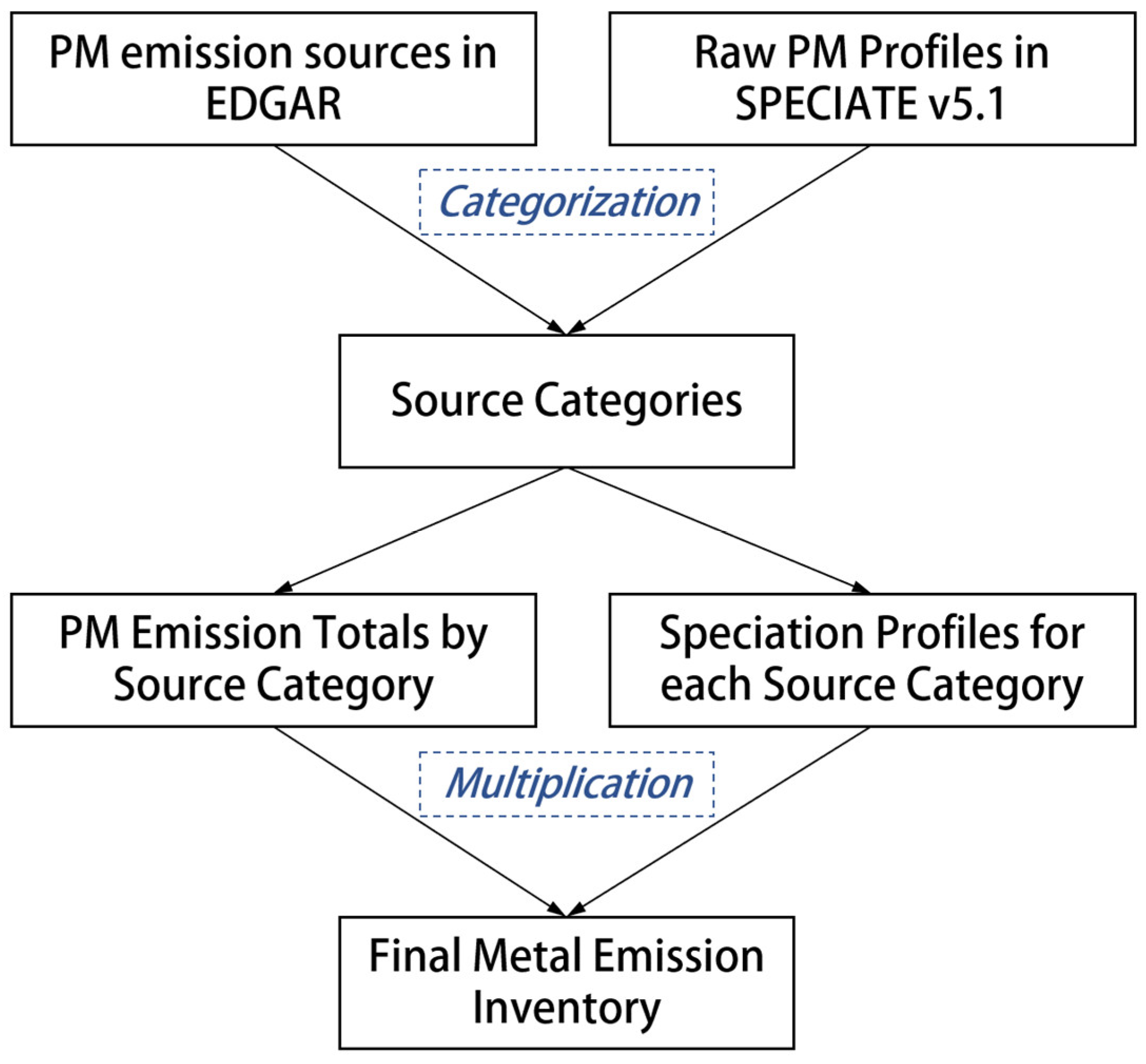
2.2. Methodology for the Establishment of Natural and Anthropogenic Emission Inventories

In this study, emission sources of metallic elements (Pb, As, Cd, and Cr) were categorized into land-based anthropogenic sources, marine-based anthropogenic sources (as known as shipping), and land-based natural dust sources to establish metal emission inventories with the base year of 2017. The metal emission inventory for land-based anthropogenic sources was established by multiplying the emission fluxes from each source in the existing bottom-up PM emission inventory by the mass fraction of metal elements in PM for the corresponding source sectors. Figure 1 contains a flow diagram of the method.

Since PM is classified into a fine mode (particle diameter < 2.5 μm) and a coarse mode (2.5 μm < particle diameter < 10 μm) and the mass fractions of metal elements differ in PM of different modes, this study organized the metal emission factors for the two particle modes and calculated the metal emission inventories separately. The global 0.1 × 0.1° gridded fine and coarse PM emission data for 2017 were obtained from the Emissions Database for Global Atmospheric Research (EDGAR) [63,64], and the mass fractions of metallic elements in PM from different emission sectors were provided by the SPECIATE v5.1 database (updated in June 2020) [65,66]. EDGAR provides worldwide emissions of GHGs as well as air pollutants such as PM, including 7 main sectors and 25 subsectors. SPECIATE is the U.S. Environmental Protection Agency’s (EPA) repository of speciation profiles on the species makeup or composition of PM and other pollutants. The profiles of PM species’ weight fractions are specific to particle-size ranges. Speciation data are developed through source testing by laboratories and research institutes and are often published in journal articles. The atomic form results are measured by an X-ray fluorescence (XRF) technique, and the ionic form results are measured by ion chromatography. This study first identified the corresponding categories in the SPECIATE database based on the emission sectors from EDGAR. Then, the median value of speciation profiles for that category was calculated and used to represent the metal emission factor of the sector. The same methodology was used in the previous metal emission inventories [62,67,68,69,70,71]. The main sectors and sub-sectors and corresponding metal emission factors for each sector are shown in

Table 1. Emission factors for metals in fine particulate matter (Unit: %).

Main Sector	Sub-Sector	Pb	As	Cd	Cr
Power Industry	Power Industry	0.04237	0.00989	0.00278	0.02659
	Fuel Exploitation	0.02192	0.05000	0.00000	0.00890
	Oil Refineries and Transformation Industry	0.01622	0.00600	0.00430	0.08534
Transport	Aviation Cruise	0.00000	0.00000	0.00000	0.02248
	Road Transportation Resuspension	0.00954	0.00161	0.00472	0.02499
	Road Transportation No Resuspension	0.12387	0.00250	0.00463	0.02645
Industrial Combustion	Combustion for Manufacturing	0.05000	0.01883	0.00220	0.00650
	Fossil-Fuel Fires	0.00670	0.01786	0.04630	0.01828
	Iron and Steel Production	0.33800	0.02440	0.03600	1.05399
	Non-ferrous Metals Production	3.99266	1.18400	0.36501	0.04058
	Non-metallic Minerals Production	0.06063	0.00287	0.00300	0.05314
Agriculture	Agricultural Waste Burning	0.03619	0.00381	0.00343	0.00236
Waste	Solid-Waste Landfills	0.00380	0.00020	0.00000	0.00540
	Solid-Waste Incineration	1.05000	0.00300	0.00300	0.01750
Buildings	Residential	0.01019	0.00096	0.00050	0.00350
Other	Chemical Processes	0.03600	0.01185	0.23400	0.10003
	Food and Paper	0.00543	0.00051	0.00458	0.00408
	Solvents and Products Use	0.04750	0.00702	0.00773	0.03063

(fine mode) and

Table 2. Emission factors for metals in coarse particulate matter (Unit: %).

Main Sector	Sub-Sector	Pb	As	Cd	Cr
Power Industry	Power Industry	0.03972	0.00087	0.01792	0.04166
	Oil Refineries and Transformation Industry	0.04010	0.00220	0.00600	0.12587
Transport	Aviation Cruise	0.00180	0.01040	0.00000	0.00000
	Road Transportation Resuspension	0.14576	0.01155	0.00008	0.02032
	Road Transportation No Resuspension	0.07749	0.00526	0.01892	0.01689
Industrial Combustion	Combustion for Manufacturing	0.11350	0.01433	0.02455	0.00857
	Fossil-Fuel Fires	0.07028	0.01033	0.02170	0.04219
	Iron and Steel Production	0.23000	0.01300	0.02958	0.32188
	Non-ferrous Metals Production	1.42406	1.15050	0.23283	0.03258
	Non-metallic Minerals Production	0.07067	0.00892	0.00597	0.03629
Agriculture	Agricultural Waste Burning	0.03644	0.00086	0.02294	0.00536
Waste	Solid-Waste Landfills	0.00510	0.00000	0.00290	0.00650
	Solid-Waste Incineration	1.05000	0.00523	0.11688	0.04988
Buildings	Residential	0.01258	0.00027	0.00000	0.00350
Other	Chemical Processes	0.01627	0.00138	0.02020	0.02088
	Food and Paper	0.00613	0.00163	0.00550	0.00338
	Solvents and Products Use	0.01334	0.00063	0.00069	0.01150

(coarse mode).

The ship metal emission inventory was calculated using a bottom-up ship emission model based on the hourly automatic identification database (AIS) data. The details of this activity-based ship emission model, the detailed information about the AIS database, and the low load-adjustment multipliers used in the calculation of ship emissions have been introduced in our previous studies [72,73,74,75]. Metal emission factors were required to calculate metal emissions from ships using the model. In this study, the emission factors of the four metallic elements were collected from several comprehensive emission measurement studies of marine engines [76,77,78,79,80,81,82,83,84,85], as presented in

Table A1. Emission factors of metals from ship sources reported in previous studies (unit: g·kWh⁻¹).

Engine Type	Fuel Type	Sulfur Content	Pb	As	Cd	Cr	Period	Reference
ME SSD	HFO	2.70	9.00 × 10−6	9.60 × 10−6	6.00 × 10−7	3.00 × 10−6	2012	Celo et al., 2015 [78]
ME SSD	HFO	2.85	3.00 × 10−6	3.00 × 10−6	5.00 × 10−5	1.00 × 10−5	2007	Agrawal et al., 2008 [76]
ME SSD	HFO	2.05	5.59 × 10−5	4.02 × 10−6	5.59 × 10−5	1.86 × 10−5	2007	Agrawal et al., 2008 [77]
ME MSD	HFO	1.48	6.00 × 10−6	1.10 × 10−6		5.00 × 10−6	2012	Celo et al., 2015 [78]
ME MSD	HFO	2.21	7.10 × 10−6	5.60 × 10−6	2.00 × 10−7	1.90 × 10−5
ME MSD	HFO	2.33	1.35 × 10−7			9.93 × 10−6	2017	Corbin et al., 2018 [79]
ME MSD	HFO	0.58				1.67 × 10−5	2010	Moldanová et al., 2013 [80]
ME MSD	HFO	0.96				1.52 × 10−5
ME MSD	HFO	2.70	8.18 × 10−5	1.34 × 10−5	5.95 × 10−6	7.44 × 10−6	2013	Sippula et al., 2014 [81]
ME MSD	HFO	0.68	2.57 × 10−6	1.54 × 10−5		1.20 × 10−5	2016	Zhang et al., 2018 [85]
ME MSD	HFO	1.60	8.50 × 10−5	1.90 × 10−5	5.40 × 10−6	2.30 × 10−5	2015	Streibel et al., 2017 [82]
ME MSD	HFO	0.48				5.40 × 10−4	2015	Zetterdahl et al., 2016 [83]
ME MSD	MDO	0.10				3.62 × 10−6	2010	Moldanová et al., 2013 [80]
ME MSD	MDO	0.13		5.93 × 10−7	7.13 × 10−6	7.42 × 10−6	2015	Zhang et al., 2016 [84]
ME HSD	MDO	0.08		4.05 × 10−4	2.22 × 10−4	3.96 × 10−5
AE MSD	MGO	0.03				3.47 × 10−5	2010	Moldanová et al., 2013 [80]
AE MSD	MGO	0.06	1.00 × 10−6	1.00 × 10−6	4.00 × 10−5	6.00 × 10−6	2007	Agrawal et al., 2008 [76]

Note: ME and AE are the main and auxiliary engines, respectively. SSD, MSD, and HSD are slow-, medium-, and high-speed diesel, respectively. HFO, MDO, and MGO are heavy fuel oil, marine diesel oil, and marine gas oil, respectively.

. According to the ship classification in the ship emission model, the power-based emission factors were categorized by engine and fuel type, as described in Appendix A. The final categorized emission factors used in this study are shown in

Table 3. Emission factors for ships used in this study (unit: g·kWh⁻¹).

Engine Type	Fuel Type	Sulfur Content	Pb	As	Cr	Cd
ME SSD	HFO	2.7%	9.00 × 10−6	5.29 × 10−6	4.74 × 10−5	9.47 × 10−6
ME MSD	HFO	2.7%	1.06 × 10−5	1.34 × 10−5	5.95 × 10−6	3.88 × 10−5
	MDO	0.5%	8.33 × 10−6	2.53 × 10−3	1.39 × 10−3	2.48 × 10−4
ME HSD	MDO	0.5%	8.33 × 10−6	8.33 × 10−6	3.33 × 10−4	3.14 × 10−4
AE MSD	MGO	0.5%	8.33 × 10−6	8.33 × 10−6	3.33 × 10−4	3.14 × 10−4

Note: ME and AE are the main and auxiliary engines, respectively. SSD, MSD, and HSD are slow-, medium-, and high-speed diesel, respectively. HFO, MDO, and MGO are heavy fuel oil, marine diesel oil, and marine gas oil, respectively.

.

Emissions of trace metals from dust sources were generated by the in-line windblown dust module during CMAQ runs. By modifying the in-line module to include metallic elements, metals can run with 20 categories of land-use data from MODIS. For the dust speciation factor, we set 0.00023 and 0.000029 for the fine and coarse mode of Pb, 0.000047 and 0.000012 for that of As, 0.0000064 and 0.00000065 for that of Cr, and 0.00019 and 0.000056 for that of Cd, respectively, based on previous studies of local measurements [86,87,88,89,90,91].

For non-trace pollutants, including sulfur dioxide (SO₂), nitrogen oxides (NO_x), carbon monoxide (CO), non-methane volatile organic compounds (NMVOCs), particulate matter (PM₁₀, PM_2.5), and ammonia (NH₃), emission inventories were calculated for both land-based anthropogenic sources and marine ship sources. For land-based anthropogenic sources, we used open-access emission inventories. In mainland China, the Multi-Resolution Emission Inventory (MEIC, http://www.meicmodel.org, accessed on 15 March 2024) in 2017 [92,93] was used, and the MIX emission data in 2010 [94] was used in Asian regions other than mainland China, both with a grid resolution of 0.25° × 0.25°. The MEIC model covers five main categories of anthropogenic emission sources in China, namely power, industrial, transport, residential, and agriculture, and uses different methods to establish emission inventories for each sector. For example, MEIC employs a unit-based method to calculate emissions from the power and industrial sectors on a facility-by-facility basis. It constructs emission inventories for the residential sector based on national-wide survey data, combined with the Energy Statistics Yearbook. It calculates emissions from the transport sector based on a high-resolution country-level vehicle emission inventory. The MIX model also covers these five emissions sources, providing emission data of pollutants and GHGs from 30 countries and regions in Asia. It was developed using a multi-scale data coupling approach, coupling and assimilating localized emission inventories such as MEIC (China), PKU-NH3 (China‘s ammonia emission inventory), CAPSS (Republic of Korea), ANL-India (India), and REAS2 (Japan, Taiwan). For ship sources, a bottom-up ship emission model based on AIS data was still used to calculate the emission inventories for these species. The description of the model and the calculated emission inventories of non-trace pollutants can be obtained from our previous studies [62,74,95].

3. Results and Discussion

3.1. Emission Inventory

3.1.1. Sector Contribution of Metal Emissions

The metal emission inventory established in this study contained three types of emission sources, namely land-based anthropogenic sources, dust sources, and ship sources, and the three sources contributed differently to the metals in the two modes of fine and coarse. As shown in Figure 2a,c, emissions from land-based anthropogenic sources were generally greater than those from ship or dust sources. The relative contribution of land-based anthropogenic sources to the fine mode emissions of Pb, As, Cd, and Cr exceeded 88% (Cr) and reached up to 93% (Pb), and the relative contribution to the coarse mode emissions exceeded 52% (Cr) and reached up to 99% (Cd). The PM emitted from dust was typically larger in particle size and thus contributed mainly to metal emissions in the coarse mode, contributing 48% of Cr and 37% of As. For metals in the fine mode, the relative contributions of dust were all below 12% (Cr) and as low as 3% (Cd). The contribution of ship sources was overall low, with the highest relative contribution occurring for Cd in the fine mode (5%), followed by As in the fine mode (2%), with very low contributions to the remaining metals.

Anthropogenic sources were the most significant sources for the emissions of metals. Based on Section 2.2, this study distinguished seven main sectors of land-based anthropogenic sources, namely power industry, industrial combustion, transport, agriculture, waste, buildings, and other. Considering that the EDGAR-based categorization standard includes shipping in the transport sector, the ship-source metal emissions calculated by this study were summarized in the transport sector. The contribution of each sector to Pb, As, Cr, and Cd is shown in Figure 2b,d. Industrial combustion was basically the most dominant anthropogenic source of all the metals, except for Cr in the coarse mode which was mainly emitted by the power industry. This is in agreement with the findings of Wang et al. (2019 [96]).

Metals emitted from industrial combustion were, in descending order, Pb (12,583 tons/year), Cr (3589 tons/year), As (2681 tons/year), and Cd (2251 tons/year), with fine modes accounting for 52%, 88%, 70%, and 22% respectively. The emissions from the power industry were also high, especially for Cr (3278 tons/year) and Pb (1652 tons/year), of which 60% of Cr and 57% of Pb were distributed in the coarse mode. In addition to these two sectors that contributed significantly to all metals, some sectors contributed to specific metals. For example, the waste sector emitted 2177 tons of Pb and 242 tons of Cd. Due to the combustion of lubricating oils in automobile engines, and the wear and tear of brake pads [97], Pb emissions from the transport sector amounted to 551 tons/year and were mainly distributed in the fine mode (67%). The agriculture sector had the highest relative contribution to the emission of Cd, amounting to 3.6%, with a total of 174 tons.

Considering the significant contribution of the industrial combustion sector to metal emissions, it has become a focus of attention for metal emission reductions. According to the study on the trend of metal emissions in China from 2012 to 2017 by Bai et al. (2023 [98]), it was found that among all emission-reduction measures, upgrading industrial boilers, raising industrial emission standards, and phasing out outdated industrial capacity are the most effective methods, accounting for 92% of the national metal emission reduction over these five years. This was also reported in the study by Zhang et al. (2019 [99]), which further emphasized the importance of promoting cleaner fuels in the residential sector as well. In the future, emission-reduction measures in the industrial combustion sector need to be continued, as it remains a major source of metal emissions. In addition to end-of-pipe emission control for industries, the role of adjusting energy structure should also be emphasized. In 2017, the base year of our emission inventory, coal still accounted for the majority of China’s energy consumption. Future policies should focus more on the introduction of renewable fuels to achieve sustained emission reductions.

There were some studies on metal emission inventories that can be used for the validation of the inventories established in this study. According to Tian et al. (2015 [100]), land-based anthropogenic sources in China emitted 2529.0 tons of As, 14,397.6 tons of Pb, and 7834.1 tons of Cr in 2012. In this study, the metal emissions from land-based anthropogenic sources in China were 2312.9 tons of As, 13,973.8 tons of Pb, and 5119.6 tons of Cr in 2017. With advances in industrial technology and Chinese air pollution prevention and control actions, it is reasonable for metal emissions to be slightly lower in 2017 than in 2012. For specific sectors, China’s Pb and Cd emissions from the iron and steel industry were 3746.0 and 39.0 tons in 2011 [101] and 2906.1 and 72.0 tons/year in this study (2017), respectively. Taking into account the differences in the base year and the categorization criteria for the emission sources, the slight differences between emission inventories do not affect the credibility of our results.

The particle size distribution of metals on atmospheric PM affects the residence time of metals in the atmosphere and influences factors such as transport distances and chemical reactions. Fine particles have a greater impact on human and animal health compared to coarse particles. This is because fine particles tend to have a longer residence time in the atmosphere, can be transported over long distances, are more easily able to penetrate indoor environments, and can even penetrate deep into the lungs [102].

Table 4. Emissions of metals in fine and coarse mode from all sources (unit: tons/year) and the ratio of fine to coarse mode.

	Pb	As	Cr	Cd
Fine Mode	10,605.38	2366.58	825.76	5468.24
Coarse Mode	8648.01	1048.90	2506.03	3911.22
Sum	19,253.39	3415.48	3331.79	9379.46
the Ratio of Fine–Coarse	1.23	2.26	0.33	1.40

shows the emissions of metals in fine and coarse mode from all three sources (land-based anthropogenic, dust, and ship sources) and the ratio of fine to coarse mode emissions. The metal with the highest distribution in the fine mode was As, with a ratio of 2.26 and a total of 2367 tons in the fine mode. On the other hand, the lowest was Cr, with a ratio of only 0.33. This indicated that the emissions of Cr in the coarse mode (2506 tons) were much higher compared to the fine mode (826 tons), and it was the only metallic element with higher emissions in the coarse mode. Pb has a more balanced distribution of particle sizes, with 10,605 tons in fine mode and 8638 tons in coarse mode, and the total emissions were the highest of the four metals. The emissions of Cd in the fine mode were 1.4 times higher than those in the coarse mode.

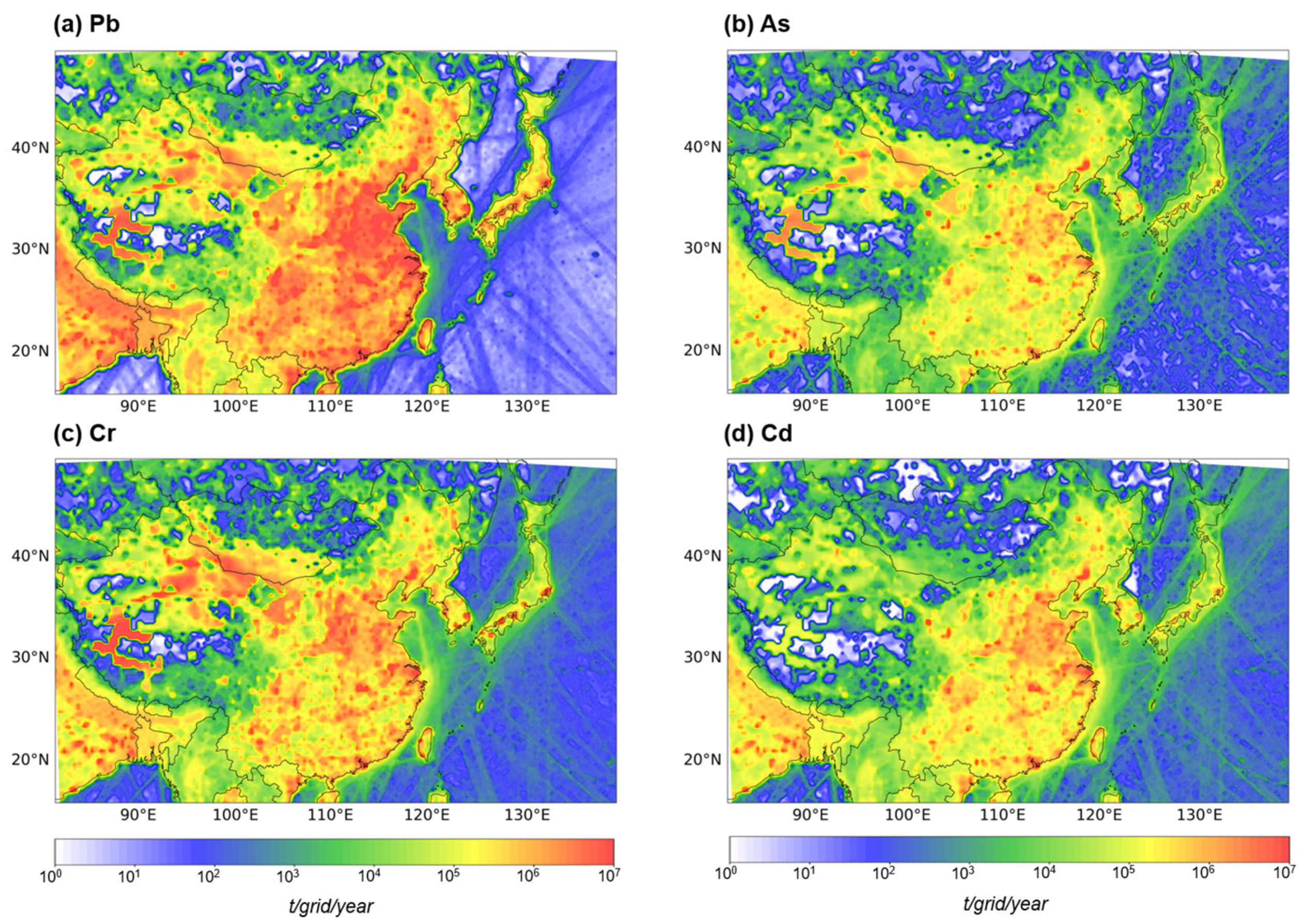
3.1.2. Spatial Distribution of Metal Emissions

In East Asia (80° E–140° E, 15° N–50° N), metal emissions were higher in Eastern China, the North China Plain, the coastal cities of Japan and Korea, and Northern India (as shown in Figure 3), which are related to the more developed industrial activities in these areas [100,103]. Since the contribution of natural dust sources was taken into account, it can be seen that in Northwestern China, as well as in Mongolia, the emissions of Cr and Pb were relatively high and comparable to those in central China. In the sea area, emissions from ships were mainly concentrated within 200 nautical miles of China, with significant emissions in the sea around Japan and Korea and also in more remote open sea areas. Metal emissions in the sea area might have an impact on air quality and even atmospheric deposition inland under the influence of sea and land breezes [62]. Especially for the elements As and Cd, the emissions from shipping were comparable to those from inland areas (e.g., Central and Southwestern China).

At the spatial scale covered by the emission inventory, land-based anthropogenic, dust, and ship sources emitted 19,253, 3415, 3332, and 9379 tons of Pb, As, Cr, and Cd, respectively. China was a significant source of metal emissions, emitting 13,868.2, 2295.4, 2328.1, and 5081.0 tons/year of Pb, As, Cr, and Cd respectively. The emissions of Pb, As, Cr, and Cd from Japan and Korea were 372.3, 38.5, 64.7, and 220.1 tons/year, from India were 2278.4, 333.0, 538.0, and 910.2 tons/year, and from Southeast Asia were 513.6, 39.7, 125.9, and 231.4 tons/year respectively. At the urban scale in China, Pb emissions from Liaoning province were high at 1232.9 tons/year, followed by Hebei (952.8 tons) and Shandong (814.4 tons) province. The emissions of As from Qinghai province were the highest at 374.7 tons/year. Qinghai is not one of the most industrially developed cities in China, but the emissions of As are strongly influenced by dust sources, and the source area of dust is distributed in northwestern China. The emissions of Cr were also significantly influenced by dust sources, with Tibet province (991.0 tons) having similar emissions to Liaoning province (877.3 tons), where heavy industry is well developed. The emissions of Cd were significant in Liaoning and Hubei provinces, with 216.1 and 170.0 tons/year, respectively, followed by Shanghai and Shandong provinces, both with about 144 tons/year.

3.2. Trace Metals in the Atmosphere

Trace metals in the atmosphere may jeopardize human and vegetation health. The United Nations Convention on Long-Range Transboundary Air Pollution has studied the atmospheric concentrations of metals in various countries around the globe, showing that China has the highest concentrations of Pb and Cd, followed by India [104]. In this study, the distribution of atmospheric concentrations of Pb, As, Cr, and Cd in East Asia (including countries such as China and India) was obtained by CMAQ v5.4 simulation. As shown in Figure 4, the concentrations of all metals were characterized by an inhomogeneous spatial distribution, which was generally consistent with the spatial distribution of the emissions of metals (Figure 3). There were areas of high atmospheric concentrations of metals in Eastern China and northern India, and relatively high metal concentrations in the marginal seas of China, such as the Bohai Sea, the Yellow Sea, and the East China Sea. Considering that PM undergoes atmospheric transport before deposition, the atmospheric concentrations over the sea area might eventually have an impact on the metal deposition fluxes in the land area as well. In mainland China, the average concentrations of Pb, As, Cr, and Cd were 7.69, 1.46, 3.53, and 1.04 ng/m³, respectively, and the highest gridded concentrations reached 792.7 ng/m³ (Liaoning province), 237.0 ng/m³ (Qinghai province), 916.1 ng/m³ (Liaoning province), and 130.5 ng/m³ (Liaoning province), respectively.

This study focused on mainland China, and the average concentrations of the four metals in 31 provinces in mainland China are shown in

Table 5. Average atmospheric metal concentrations in the provinces of mainland China (unit: ng/m³).

Province	Pb	As	Cr	Cd
Beijing	49.25	5.52	27.87	7.58
Tianjin	37.79	4.65	13.16	5.63
Hebei	19.20	2.52	8.26	2.74
Shanxi	16.62	3.30	9.88	2.29
Inner Mongolia	3.11	0.85	1.43	0.42
Liaoning	35.68	5.81	32.58	5.35
Jilin	6.40	1.00	3.63	0.83
Heilongjiang	3.37	0.50	1.58	0.42
Shanghai	20.37	2.52	19.49	3.38
Jiangsu	32.60	4.31	15.06	4.82
Zhejiang	18.84	2.60	9.11	2.70
Anhui	22.21	3.12	9.85	3.10
Fujian	7.88	1.16	2.99	1.10
Jiangxi	11.69	1.68	5.27	1.55
Shandong	27.08	3.74	8.69	3.76
Henan	23.36	3.46	7.39	3.18
Hubei	25.36	3.65	18.10	3.74
Hunan	12.88	1.82	5.84	1.67
Guangdong	11.55	1.46	3.76	1.67
Guangxi	12.87	3.54	2.97	1.57
Hainan	6.10	0.86	2.29	0.80
Chongqing	12.16	1.66	4.14	1.65
Sichuan	6.74	0.96	2.15	0.93
Guizhou	9.30	2.34	2.56	1.14
Yunnan	3.60	0.54	1.66	0.48
Tibet	0.32	0.07	0.31	0.02
Shaanxi	14.61	4.50	3.18	1.82
Gansu	8.33	3.01	1.67	0.99
Qinghai	3.88	1.71	0.70	0.42
Ningxia	7.06	1.63	2.68	1.01
Xinjiang	1.58	0.34	1.28	0.19

. The emissions of Pb, As, Cr, and Cd were highly correlated with the industrial combustion sectors, and therefore, the concentrations of these metals may be 2–10 times higher in Northern, Eastern, and parts of Western China (especially in the Beijing–Tianjin–Hebei region, Shandong, Jiangsu, Shanghai, Sichuan, and Shaanxi provinces) than in other regions. In 2017, the concentrations of Pb were high in Eastern China, Central China, and parts of Western China, especially in Beijing, Tianjin, Liaoning, Shandong, and Jiangsu provinces, with average concentrations as high as 27.10–49.25 ng/m³. In contrast, the lowest concentration of Pb occurred in Tibet, at 0.32 ng/m³. The concentrations of Cr were second to Pb, with high concentrations in Beijing–Tianjin–Hebei, and also in the Yangtze River delta, reaching 15.06–32.58 ng/m³, and the lowest concentration also occurred in Tibet (0.31 ng/m³). The differences in the concentrations of As and Cd among different cities were relatively small, ranging from 0.07–5.81 ng/m³ and 0.02–7.58 ng/m³, respectively, with the highest concentrations occurring in Liaoning and Beijing. Overall, metal concentrations were relatively high in Liaoning, the Beijing–Tianjin-Hebei region, and Eastern China (Jiangsu, Shanghai, and Shandong), and low in Tibet and Xinjiang.

3.3. Atmospheric Deposition of Trace Metals

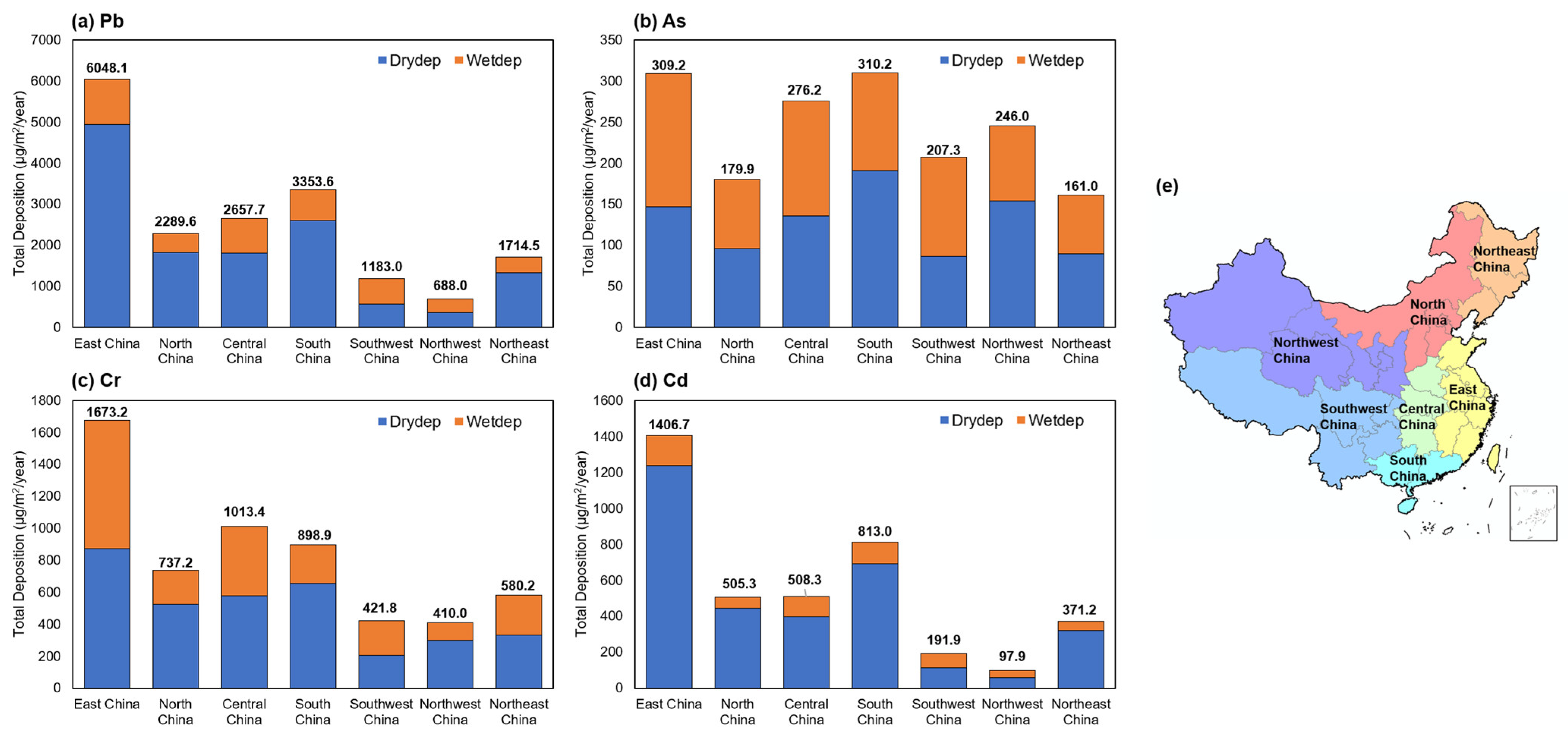
3.3.1. Dry and Wet Deposition

Trace metals bound to PM eventually accumulate on land through the process of dry and wet deposition [32,33]. Dry deposition is defined as the direct deposition of atmospheric particles on the surface in the absence of snowfall or rainfall events [105,106]. And dry deposition of atmospheric PM is a potentially important source of pollutants on the surfaces of water bodies, soils, or plants [107,108,109]. Wet deposition is a precipitation-induced process involving the binding of PM to water droplets in and under clouds [110,111]. During precipitation, fine particles of anthropogenic sources get wiped away due to nucleation where aerosols or droplets get in the way. In contrast, coarse particles of crustal origin get scavenged below the clouds during precipitation [112]. In summary, atmospheric particles are deposited on the surface during rainfall or snowfall after dissolving in clouds and attaching to precipitation droplets [105,113]. Different metallic elements come from dry and wet deposition in different proportions and have different spatial distribution patterns. In this study, the spatial distribution of dry and wet deposition of four metals, Pb, As, Cr, and Cd, in mainland China were plotted in Figure 5 and Figure 6, respectively.

Since dry deposition is less influenced by meteorological conditions (precipitation, pH, etc.), it is a function of atmospheric concentration and the rate of dry deposition of PM. Therefore, high dry-deposition fluxes were present in areas with high emissions [108], with a spatial distribution pattern similar to that of emissions (Figure 3) and atmospheric concentrations (Figure 4) of metals. The high values of deposition fluxes were mainly distributed in Eastern and Northern China. The difference was that, for Cr, As, and Pb, there were significant dry-deposition fluxes in the dust source regions of China (Gobi Desert, Taklamakan Desert, and Loess Plateau [114]). The residence time of particles in the atmosphere depends largely on the particle size [115], and therefore, the dry deposition rate of coarse particles is higher than that of fine particles [116]. Due to their larger particle sizes and higher dry-deposition rates, dust particles are more susceptible to removal from the atmosphere through dry deposition. As a result, metallic elements emitted by dust tend to quickly return to the surface once they are released into the atmosphere. In contrast, Cd did not show such distribution characteristics, which had a very low contribution from dust sources. This confirmed our inference that the dry deposition of metals in Northwest China was mainly from dust sources. In mainland China, the average dry-deposition fluxes of Pb, As, Cr, and Cd were 668.2, 95.9, 299.5, and 138.0 μg/m², respectively, and the maximum gridded dry-deposition fluxes were 98.4 mg/m² (Shanghai), 17.8 mg/m² (Guangxi), 18.3 mg/m² (Hubei), and 25.1 mg/m² (Shanghai), respectively.

Unlike the spatial distribution of dry deposition, the spatial distribution of wet-deposition fluxes of metals showed significant differences compared to that of emissions and atmospheric concentrations. Because wet deposition is a precipitation-related process, fine PM is more likely to become a condensation nucleus for wet deposition and then be removed from the atmosphere. Fine PM tends to undergo prolonged atmospheric transport and is more characterized by regional transport [46]. So, the spatial distribution of wet deposition reflected the movement of atmospheric PM after it was emitted into the air, and illustrated the influence of factors other than gravity on the deposition of metals. A study by Sakata et al. (2006 [117]) demonstrated the contribution of long-range transport of PM released from the Asian continent to the wet-deposition fluxes of Pb, As, and Cd in Japan. For mainland China, the deposition fluxes were high in Eastern, Central, and also Southwestern China. Furthermore, the deposition fluxes were higher in the south than in the north, a trend also reported in a previous study [117], owing to the correlation of wet deposition with precipitation. Metals emitted from dust sources were predominantly distributed in the coarse mode and made minimal contributions to wet deposition, resulting in insignificant wet-deposition fluxes of the four metals in and near the dust source areas. In China, the average wet-deposition fluxes of Pb, As, Cr, and Cd were 368.3, 74.4, 166.4, and 47.0 μg/m², respectively, and the maximum gridded wet-deposition fluxes were 13.7 mg/m² (Guangxi), 7.1 mg/m² (Guangxi), 12.2 mg/m² (Shanghai), and 2.0 mg/m² (Shanghai), respectively.

3.3.2. Bulk Deposition

Regardless of dry or wet deposition, the total amount of metals ultimately input to the soil is determined by atmospheric bulk deposition. In mainland China, the average bulk-deposition fluxes of Pb, As, Cr, and Cd were 1036.5, 170.3, 465.9, and 185.0 μg/m², respectively, and the maximum gridded bulk-deposition fluxes were 110.6 mg/m² (Shanghai), 24.9 mg/m² (Guangxi), 25.1 mg/m² (Hubei), and 27.1 mg/m² (Shanghai), respectively.

According to Figure 7e, China was divided into seven regions, namely Northeast China, North China, Northwest China, East China, Central China, Southwest China, and South China. The total dry and wet deposition of the four metals was counted for each of the seven regions (as shown in Figure 7a–d).

The percentage of dry and wet deposition (dry or wet deposition fluxes divided by bulk-deposition fluxes) varied for different metals. For As, the percentage of wet deposition was higher throughout China, reaching an average of 47%, and up to 58% in Southwest China. The difference in the contribution of trace metals from dry and wet deposition may be due to the different particle size distributions of these metal elements. Coarse mode particles have a much shorter lifetime in the atmosphere due to higher deposition rates and do not significantly act as condensation nuclei for precipitation formation. As a result, the dry-deposition fluxes of trace metals associated with larger particles are greater than their wet-deposition fluxes [117]. Based on the discussion in Section 3.1.1, it was found that the size distribution of As was the highest in the fine mode, which explained the largest proportion of wet deposition. However, the emissions of Cr had the lowest percentage of fine mode and still had a high average proportion of wet deposition (38%), especially in Southwest China, where the proportion reached 51%. The results of Ye et al. (2018 [118]) showed that the particle size distribution of heavy metals in atmospheric aerosols varies from region to region. Although there was a higher percentage of Cr elements in the fine mode throughout the whole simulation region, data on the particle size distribution of the metals were insufficient at smaller scales, so this part of the study needs further refinement. For all four metals, the percentage of wet deposition was highest in Southwest China, which was related to the higher relative humidity and precipitation in this region [119]. Sakata and Asakura (2011 [120]) also showed that wet deposition was the main way of atmospheric deposition in monsoon regions with abundant precipitation. However, there is a significant seasonal variation in wet deposition, which is higher in seasons with frequent precipitation, while dry deposition is stable in all seasons [120]. Overall, dry deposition is the dominant mode of metal deposition on time scales of years and beyond.

Almost all metals had the highest bulk-deposition fluxes in East China, which was in agreement with the results of previous studies [19,52]. Metal emissions were high in East China, and because this study considered marine emission sources, the eastern coast of China was affected by both continental and marine sources of emissions. Pb, Cr, and Cd, except for As, all had the lowest bulk-deposition fluxes in Northwest China. Since the emissions of As were strongly influenced by dust sources, and the distribution of dust source areas in China are in the Northwest, resulting in the lowest depositional fluxes of As not being in that region. Influenced by intensive smelting activities [46,121], Central China had high bulk-deposition fluxes. For example, the bulk-deposition fluxes of Pb, As, Cd, and Cr in Hunan province were 12.24, 0.30, 0.39, and 0.90 mg/m²/year, respectively, which were similar to the measured results of Feng et al. (2019 [122]). South China also had intensive non-ferrous and non-metallic mineral-mining activities [50,118,122,123], which similarly resulted in high bulk-deposition fluxes in that region. The bulk-deposition fluxes of Pb, As, Cd, and Cr in Guizhou province were 1.65, 0.42, 0.26, and 0.51 mg/m²/year, respectively, which were similar to the measured results of Lin et al. (2022 [124]). A similar pattern was shown in a previous study [125], with higher metal-deposition fluxes in South–Central China than in Northern China.

3.4. Limitations of This Study

The metal emission inventory developed in this study used the EDGAR and SPECIATE databases to calculate emissions of metals from land-based anthropogenic sources. However, the emission factors used in the EDGAR database for global PM emissions are based primarily on the air-pollutant emission inventory guidebook of the European Environment Agency (EEA), which are mainly measured in North America and Europe. Developing countries tend to have higher emission factors than developed countries because of the asynchronous application of end-of-pipe treatment technologies or industrial production technologies. To mitigate uncertainties in emission inventories, continuous updates are necessary for determining emission factors in developing countries. Although SPECIATE has a rigorous system for assessing data quality, its wealth of data sources, including the literature and institutional measurements [65], inevitably leads to inconsistencies in measurement standards. It should be noted that the emission factors ultimately used in this study are the median values of each emission sector in the SPECIATE database, minimizing the impact of extreme data and controlling the uncertainties as much as possible. For ship emissions, a model based on the AIS database and ship emission factors collected from the literature were employed. Research results on metal element analysis of PM emitted from ships are limited, and many studies have been conducted on local ships in European and American countries. Ships in different regions and countries use different types of fuels. Therefore, using elemental measurement results from European and American countries to calculate ship emissions in East Asia may introduce some uncertainties. On the one hand, there is a need to enhance the measurements of emission factors in various regions. On the other hand, it is necessary to establish internationally recognized testing standards to ensure the accuracy and universality of emission-factor testing.

In this study, the CMAQ model was modified to include metallic elements as tracers, which are considered inert elements for the simulation of atmospheric concentration and atmospheric deposition. However, during atmospheric transport, metallic elements may undergo chemical reactions with inorganic ions in aerosols, and they may also change forms under different pH and humidity conditions, thus affecting their atmospheric concentrations and deposition fluxes. This study innovatively incorporated metallic elements into the modified CMAQ model. But in the future, it is necessary to consider the chemical processes of the metallic elements and to refine the chemical mechanisms of metals in the model.

4. Conclusions

Natural and anthropogenic sources influence trace metals bound to different-sized PM in dry and wet atmospheric deposition. In the long run, this may result in contamination of the soil environment, which in turn affects human health. Emission inventories of trace metals that include both natural and anthropogenic sources have yet to be studied. Due to the difficulty of providing concentration and deposition flux data over large spatial scales from field monitoring, numerical models offer the possibility of solving this problem. In this study, emission inventories of four metallic elements (Pb, As, Cr, and Cd) in East Asia (80° E–140° E, 15° N–50° N) were established, and gridded data on emissions, concentrations, and dry and wet atmospheric deposition of Pb, As, Cr, and Cd were provided by the modified CMAQ model. The analysis focused on the contribution of different emission sources to trace metals, the spatial distribution of metal emissions, atmospheric concentrations, and wet and dry deposition in mainland China, as well as the characteristics of wet and dry deposition in different regions of China.

Emissions of Pb, As, Cr, and Cd in East Asia were 19,253, 3415, 3332, and 9379 tons in 2017, with 55%, 69%, 25%, and 58% distributed in the fine mode, respectively. Industrial combustion was the most important source of emissions for all four metals, followed by the power industry. They are important for reducing metal emissions through industrial boiler upgrades and energy transformation. In mainland China, the emissions of trace metals were high in Liaoning and Shandong province. Emissions of As and Cr, which were strongly influenced by dust sources, were also significant in Tibet. The spatial distributions of both atmospheric concentrations and dry deposition of metals were similar to that of emissions, mainly in Liaoning province, the Beijing–Tianjin–Hebei region, and Eastern China (Jiangsu, Shanghai, and Shandong province). However, differences were shown in the dust source regions. Atmospheric concentrations of metals in this region were not as significant as emissions and dry deposition because coarse PM settled more readily. Metals in fine mode are transported over longer distances and are more susceptible to wet deposition, so the overall spatial distribution of wet deposition of metals was more easterly. Therefore, it is necessary to take countries, regions, and even oceans around the study area into account when considering wet-deposition fluxes of metals. Wet-deposition fluxes were greater in the south than in the north, due to the fact that wet deposition is associated with precipitation. The ratio of dry to wet deposition of metals varied, which is influenced by many factors. In general, metallic elements with a greater distribution in the fine mode and higher solubility are more readily removed from the atmosphere by wet deposition. Among the four metals covered in this study, Arsenic had the highest percentage of fine mode and also had the largest proportion of wet deposition (43.7%). The dry to wet deposition ratios of the remaining three metals were 2.91 (Cd), 1.80 (Pb), and 1.80 (Cr). In mainland China, the average bulk-deposition fluxes of Pb, As, Cr, and Cd were 1036.5, 170.3, 465.9, and 185.0 μg/m², respectively. Our study provides gridded data in mainland China of trace metals for assessing air quality, human exposure risks, and metal inputs to soils.

References

1. Manisalidis, I.; Stavropoulou, E.; Stavropoulos, A.; Bezirtzoglou, E. Environmental and health impacts of air pollution: A review. Front. Public Health 2020, 8, 14. [Google Scholar] [CrossRef]
2. Weerasundara, L.; Vithanage, M. The challenge of vehicular emission and atmospheric deposition: From air to water. Int. J. Energy Environ. Econ. 2015, 23, 603. [Google Scholar]
3. Amodio, M.; Catino, S.; Dambruoso, P.R.; de Gennaro, G.; Di Gilio, A.; Giungato, P.; Laiola, E.; Marzocca, A.; Mazzone, A.; Sardaro, A.; et al. Atmospheric Deposition: Sampling Procedures, Analytical Methods, and Main Recent Findings from the Scientific Literature. Adv. Meteorol. 2014, 2014, 161730. [Google Scholar] [CrossRef]
4. Karim, Z.; Qureshi, B.A.; Mumtaz, M.; Qureshi, S. Heavy metal content in urban soils as an indicator of anthropogenic and natural influences on landscape of Karachi—A multivariate spatio-temporal analysis. Ecol. Indic. 2014, 42, 20–31. [Google Scholar] [CrossRef]
5. Duan, J.; Tan, J. Atmospheric heavy metals and Arsenic in China: Situation, sources and control policies. Atmos. Environ. 2013, 74, 93–101. [Google Scholar] [CrossRef]
6. Hou, D.; O’Connor, D.; Igalavithana, A.D.; Alessi, D.S.; Luo, J.; Tsang, D.C.W.; Sparks, D.L.; Yamauchi, Y.; Rinklebe, J.; Ok, Y.S. Metal contamination and bioremediation of agricultural soils for food safety and sustainability. Nat. Rev. Earth Environ. 2020, 1, 366–381. [Google Scholar] [CrossRef]
7. Tchounwou, P.B.; Yedjou, C.G.; Patlolla, A.K.; Sutton, D.J. Heavy metal toxicity and the environment. In Molecular, Clinical and Environmental Toxicology; Springer Basel: Basel, Germany, 2012; Volume 3, pp. 133–164. [Google Scholar]
8. Yan, X.; Gao, D.; Zhang, F.; Zeng, C.; Xiang, W.; Zhang, M. Relationships between Heavy Metal Concentrations in Roadside Topsoil and Distance to Road Edge Based on Field Observations in the Qinghai-Tibet Plateau, China. Int. J. Environ. Res. Public Health 2013, 10, 762–775. [Google Scholar] [CrossRef]
9. Fu, S.; Wei, C.Y. Multivariate and spatial analysis of heavy metal sources and variations in a large old antimony mine, China. J. Soils Sediments 2013, 13, 106–116. [Google Scholar] [CrossRef]
10. Wei, B.; Yang, L. A review of heavy metal contaminations in urban soils, urban road dusts and agricultural soils from China. Microchem. J. 2010, 94, 99–107. [Google Scholar] [CrossRef]
11. Vardhan, K.H.; Kumar, P.S.; Panda, R.C. A review on heavy metal pollution, toxicity and remedial measures: Current trends and future perspectives. J. Mol. Liq. 2019, 290, 111197. [Google Scholar] [CrossRef]
12. Noli, F.; Tsamos, P. Concentration of heavy metals and trace elements in soils, waters and vegetables and assessment of health risk in the vicinity of a lignite-fired power plant. Sci. Total Environ. 2016, 563–564, 377–385. [Google Scholar] [CrossRef] [PubMed]
13. Bi, X.; Feng, X.; Yang, Y.; Qiu, G.; Li, G.; Li, F.; Liu, T.; Fu, Z.; Jin, Z. Environmental contamination of heavy metals from zinc smelting areas in Hezhang County, western Guizhou, China. Environ. Int. 2006, 32, 883–890. [Google Scholar] [CrossRef] [PubMed]
14. Wang, Y.; Cheng, K.; Wu, W.; Tian, H.; Yi, P.; Zhi, G.; Fan, J.; Liu, S. Atmospheric emissions of typical toxic heavy metals from open burning of municipal solid waste in China. Atmos. Environ. 2017, 152, 6–15. [Google Scholar] [CrossRef]
15. Zhang, F.; Yan, X.; Zeng, C.; Zhang, M.; Shrestha, S.; Devkota, L.P.; Yao, T. Influence of Traffic Activity on Heavy Metal Concentrations of Roadside Farmland Soil in Mountainous Areas. Int. J. Environ. Res. Public Health 2012, 9, 1715–1731. [Google Scholar] [CrossRef]
16. Ogunkunle, C.O.; Fatoba, P.O. Pollution Loads and the Ecological Risk Assessment of Soil Heavy Metals around a Mega Cement Factory in Southwest Nigeria. Pol. J. Environ. Stud. 2013, 22, 487–493. [Google Scholar]
17. Luo, C.; Liu, C.; Wang, Y.; Liu, X.; Li, F.; Zhang, G.; Li, X. Heavy metal contamination in soils and vegetables near an e-waste processing site, south China. J. Hazard. Mater. 2011, 186, 481–490. [Google Scholar] [CrossRef]
18. Nriagu, J.O. Global Metal Pollution: Poisoning the Biosphere? Environ. Sci. Policy Sustain. Dev. 1990, 32, 7–33. [Google Scholar] [CrossRef]
19. Chen, L.; Zhou, S.; Wu, S.; Wang, C.; He, D. Concentration, fluxes, risks, and sources of heavy metals in atmospheric deposition in the Lihe River watershed, Taihu region, eastern China. Environ. Pollut. 2019, 255, 113301. [Google Scholar] [CrossRef] [PubMed]
20. Vithanage, M.; Bandara, P.C.; Novo, L.A.B.; Kumar, A.; Ambade, B.; Naveendrakumar, G.; Ranagalage, M.; Magana-Arachchi, D.N. Deposition of trace metals associated with atmospheric particulate matter: Environmental fate and health risk assessment. Chemosphere 2022, 303, 135051. [Google Scholar] [CrossRef]
21. MEP; MLR. The Report on the National General Survey of Soil Contamination; Ministry of Environmental Protection & Ministry of Land and Resources: Beijing, China, 2014. [Google Scholar]
22. Hou, D.; Li, F. Complexities Surrounding China’s Soil Action Plan. Land Degrad. Dev. 2017, 28, 2315–2320. [Google Scholar] [CrossRef]
23. Hu, Y.; Cheng, H.; Tao, S. The Challenges and Solutions for Cadmium-contaminated Rice in China: A Critical Review. Environ. Int. 2016, 92–93, 515–532. [Google Scholar] [CrossRef]
24. Dong, J.; Wu, F.; Zhang, G. Influence of cadmium on antioxidant capacity and four microelement concentrations in tomato seedlings (Lycopersicon esculentum). Chemosphere 2006, 64, 1659–1666. [Google Scholar] [CrossRef]
25. Römkens, P.F.A.M.; Guo, H.Y.; Chu, C.L.; Liu, T.S.; Chiang, C.F.; Koopmans, G.F. Prediction of Cadmium uptake by brown rice and derivation of soil–plant transfer models to improve soil protection guidelines. Environ. Pollut. 2009, 157, 2435–2444. [Google Scholar] [CrossRef]
26. Sriprachote, A.; Kanyawongha, P.; Ochiai, K.; Matoh, T. Current situation of cadmium-polluted paddy soil, rice and soybean in the Mae Sot District, Tak Province, Thailand. Soil Sci. Plant Nutr. 2012, 58, 349–359. [Google Scholar] [CrossRef]
27. Sun, Y.; Sun, G.; Xu, Y.; Wang, L.; Liang, X.; Lin, D. Assessment of sepiolite for immobilization of cadmium-contaminated soils. Geoderma 2013, 193–194, 149–155. [Google Scholar] [CrossRef]
28. Tchounwou, P.B.; Patlolla, A.K.; Centeno, J.A. Invited Reviews: Carcinogenic and Systemic Health Effects Associated with Arsenic Exposure—A Critical Review. Toxicol. Pathol. 2003, 31, 575–588. [Google Scholar] [CrossRef]
29. Raj, K.; Das, A.P. Lead pollution: Impact on environment and human health and approach for a sustainable solution. Environ. Chem. Ecotoxicol. 2023, 5, 79–85. [Google Scholar] [CrossRef]
30. Atsdr, U. Toxicological Profile for Chromium; US Department of Health and Human Services, Public Health Service: Washington, DC, USA, 2012. [Google Scholar]
31. IARC. Chromium, nickel and welding. In IARC Monographs on the Evaluation of Carcinogenic Risks to Humans; International Agency for Research on Cancer: Lyon, France, 1990; Volume 49. [Google Scholar]
32. Altaf, R.; Altaf, S.; Hussain, M.; Shah, R.U.; Ullah, R.; Ullah, M.I.; Rauf, A.; Ansari, M.J.; Alharbi, S.A.; Alfarraj, S.; et al. Heavy metal accumulation by roadside vegetation and implications for pollution control. PLoS ONE 2021, 16, e0249147. [Google Scholar] [CrossRef] [PubMed]
33. Zgłobicki, W.; Telecka, M.; Skupiński, S.; Pasierbińska, A.; Kozieł, M. Assessment of heavy metal contamination levels of street dust in the city of Lublin, E Poland. Environ. Earth Sci. 2018, 77, 774. [Google Scholar] [CrossRef]
34. Kara, M.; Dumanoglu, Y.; Altiok, H.; Elbir, T.; Odabasi, M.; Bayram, A. Seasonal and spatial variations of atmospheric trace elemental deposition in the Aliaga industrial region, Turkey. Atmos. Res. 2014, 149, 204–216. [Google Scholar] [CrossRef]
35. Mijić, Z.; Stojić, A.; Perišić, M.; Rajšić, S.; Tasić, M.; Radenković, M.; Joksić, J. Seasonal variability and source apportionment of metals in the atmospheric deposition in Belgrade. Atmos. Environ. 2010, 44, 3630–3637. [Google Scholar] [CrossRef]
36. Lu, A.; Wang, J.; Qin, X.; Wang, K.; Han, P.; Zhang, S. Multivariate and geostatistical analyses of the spatial distribution and origin of heavy metals in the agricultural soils in Shunyi, Beijing, China. Sci. Total Environ. 2012, 425, 66–74. [Google Scholar] [CrossRef] [PubMed]
37. Nicholson, F.A.; Smith, S.R.; Alloway, B.J.; Carlton-Smith, C.; Chambers, B.J. An inventory of heavy metals inputs to agricultural soils in England and Wales. Sci. Total Environ. 2003, 311, 205–219. [Google Scholar] [CrossRef] [PubMed]
38. Nziguheba, G.; Smolders, E. Inputs of trace elements in agricultural soils via phosphate fertilizers in European countries. Sci. Total Environ. 2008, 390, 53–57. [Google Scholar] [CrossRef] [PubMed]
39. He, B.; Yun, Z.; Shi, J.; Jiang, G. Research progress of heavy metal pollution in China: Sources, analytical methods, status, and toxicity. Chin. Sci. Bull. 2013, 58, 134–140. [Google Scholar] [CrossRef]
40. Liu, X.; Wu, J.; Xu, J. Characterizing the risk assessment of heavy metals and sampling uncertainty analysis in paddy field by geostatistics and GIS. Environ. Pollut. 2006, 141, 257–264. [Google Scholar] [CrossRef]
41. Rogan, N.; Serafimovski, T.; Dolenec, M.; Tasev, G.; Dolenec, T. Heavy metal contamination of paddy soils and rice (Oryza sativa L.) from Kočani Field (Macedonia). Environ. Geochem. Health 2009, 31, 439–451. [Google Scholar] [CrossRef]
42. Luo, X.; Bing, H.; Luo, Z.; Wang, Y.; Jin, L. Impacts of atmospheric particulate matter pollution on environmental biogeochemistry of trace metals in soil-plant system: A review. Environ. Pollut. 2019, 255, 113138. [Google Scholar] [CrossRef]
43. Weerasundara, L.; Magana-Arachchi, D.N.; Ziyath, A.M.; Goonetilleke, A.; Vithanage, M. Health risk assessment of heavy metals in atmospheric deposition in a congested city environment in a developing country: Kandy City, Sri Lanka. J. Environ. Manag. 2018, 220, 198–206. [Google Scholar] [CrossRef]
44. Shi, T.; Ma, J.; Wu, X.; Ju, T.; Lin, X.; Zhang, Y.; Li, X.; Gong, Y.; Hou, H.; Zhao, L.; et al. Inventories of heavy metal inputs and outputs to and from agricultural soils: A review. Ecotoxicol. Environ. Saf. 2018, 164, 118–124. [Google Scholar] [CrossRef]
45. Tian, S.L.; Pan, Y.P.; Wang, Y.S. Size-resolved source apportionment of particulate matter in urban Beijing during haze and non-haze episodes. Atmos. Chem. Phys. 2016, 16, 1–19. [Google Scholar] [CrossRef]
46. Xiao, X.; Qin, K.; Sun, X.; Hui, W.; Yuan, L.; Wu, L. Will wheat be damaged by heavy metals on exposure to coal fly ash? Atmos. Pollut. Res. 2018, 9, 814–821. [Google Scholar] [CrossRef]
47. Gui, K.; Yao, W.; Che, H.; An, L.; Zheng, Y.; Li, L.; Zhao, H.; Zhang, L.; Zhong, J.; Wang, Y.; et al. Record-breaking dust loading during two mega dust storm events over northern China in March 2021: Aerosol optical and radiative properties and meteorological drivers. Atmos. Chem. Phys. 2022, 22, 7905–7932. [Google Scholar] [CrossRef]
48. Kupka, D.; Kania, M.; Pietrzykowski, M.; Łukasik, A.; Gruba, P. Multiple Factors Influence the Accumulation of Heavy Metals (Cu, Pb, Ni, Zn) in Forest Soils in the Vicinity of Roadways. Water Air Soil Pollut. 2021, 232, 194. [Google Scholar] [CrossRef]
49. Farahani, V.J.; Soleimanian, E.; Pirhadi, M.; Sioutas, C. Long-term trends in concentrations and sources of PM2.5–bound metals and elements in central Los Angeles. Atmos. Environ. 2021, 253, 118361. [Google Scholar] [CrossRef]
50. Wu, Y.; Zhang, J.; Ni, Z.; Liu, S.; Jiang, Z.; Huang, X. Atmospheric deposition of trace elements to Daya Bay, South China Sea: Fluxes and sources. Mar. Pollut. Bull. 2018, 127, 672–683. [Google Scholar] [CrossRef]
51. McNeill, J.; Snider, G.; Weagle, C.L.; Walsh, B.; Bissonnette, P.; Stone, E.; Abboud, I.; Akoshile, C.; Anh, N.X.; Balasubramanian, R.; et al. Large global variations in measured airborne metal concentrations driven by anthropogenic sources. Sci. Rep. 2020, 10, 21817. [Google Scholar] [CrossRef]
52. Li, W.; Xu, B.; Song, Q.; Liu, X.; Xu, J.; Brookes, P.C. The identification of ‘hotspots’ of heavy metal pollution in soil–rice systems at a regional scale in eastern China. Sci. Total Environ. 2014, 472, 407–420. [Google Scholar] [CrossRef] [PubMed]
53. Xu, L.; Pye, H.O.T.; He, J.; Chen, Y.; Murphy, B.N.; Ng, N.L. Experimental and model estimates of the contributions from biogenic monoterpenes and sesquiterpenes to secondary organic aerosol in the southeastern United States. Atmos. Chem. Phys. 2018, 18, 12613–12637. [Google Scholar] [CrossRef]
54. Amedro, D.; Berasategui, M.; Bunkan, A.J.C.; Pozzer, A.; Lelieveld, J.; Crowley, J.N. Kinetics of the OH + NO2 reaction: Effect of water vapour and new parameterization for global modelling. Atmos. Chem. Phys. 2020, 20, 3091–3105. [Google Scholar] [CrossRef]
55. Sarwar, G.; Gantt, B.; Foley, K.; Fahey, K.; Spero, T.L.; Kang, D.; Mathur, R.; Foroutan, H.; Xing, J.; Sherwen, T.; et al. Influence of bromine and iodine chemistry on annual, seasonal, diurnal, and background ozone: CMAQ simulations over the Northern Hemisphere. Atmos. Environ. 2019, 213, 395–404. [Google Scholar] [CrossRef]
56. Lana, A.; Bell, T.G.; Simó, R.; Vallina, S.M.; Ballabrera-Poy, J.; Kettle, A.J.; Dachs, J.; Bopp, L.; Saltzman, E.S.; Stefels, J.; et al. An updated climatology of surface dimethlysulfide concentrations and emission fluxes in the global ocean. Glob. Biogeochem. Cycles 2011, 25, GB1004. [Google Scholar] [CrossRef]
57. US EPA. CMAQ Model Version 5.3 Input Data—1/1/2016–12/31/2016 12km CONUS, 1st ed.; UNC Dataverse: Chapel Hill, NC, USA, 2019. [Google Scholar] [CrossRef]
58. Pleim, J.E. A Combined Local and Nonlocal Closure Model for the Atmospheric Boundary Layer. Part I: Model Description and Testing. J. Appl. Meteorol. Climatol. 2007, 46, 1383–1395. [Google Scholar] [CrossRef]
59. Xiu, A.; Pleim, J.E. Development of a Land Surface Model. Part I: Application in a Mesoscale Meteorological Model. J. Appl. Meteorol. 2001, 40, 192–209. [Google Scholar] [CrossRef]
60. Clough, S.A.; Shephard, M.W.; Mlawer, E.J.; Delamere, J.S.; Iacono, M.J.; Cady-Pereira, K.; Boukabara, S.; Brown, P.D. Atmospheric radiative transfer modeling: A summary of the AER codes. J. Quant. Spectrosc. Radiat. Transf. 2005, 91, 233–244. [Google Scholar] [CrossRef]
61. Kain, J.S. The Kain–Fritsch Convective Parameterization: An Update. J. Appl. Meteorol. 2004, 43, 170–181. [Google Scholar] [CrossRef]
62. Zhao, J.; Zhang, Y.; Xu, H.; Tao, S.; Wang, R.; Yu, Q.; Chen, Y.; Zou, Z.; Ma, W. Trace Elements From Ocean-Going Vessels in East Asia: Vanadium and Nickel Emissions and Their Impacts on Air Quality. J. Geophys. Res. Atmos. 2021, 126, e2020JD033984. [Google Scholar] [CrossRef]
63. Centre, J.R. Global Emission Inventories in the Emission Database for Global Atmospheric Research (EDGAR)—Manual (I); Joint Research Centre: Ispra, Italy, 2012. [Google Scholar]
64. Crippa, M.; Solazzo, E.; Huang, G.; Guizzardi, D.; Koffi, E.; Muntean, M.; Schieberle, C.; Friedrich, R.; Janssens-Maenhout, G. High resolution temporal profiles in the Emissions Database for Global Atmospheric Research. Sci. Data 2020, 7, 121. [Google Scholar] [CrossRef]
65. Bray, C.D.; Strum, M.; Simon, H.; Riddick, L.; Kosusko, M.; Menetrez, M.; Hays, M.D.; Rao, V. An assessment of important SPECIATE profiles in the EPA emissions modeling platform and current data gaps. Atmos. Environ. 2019, 207, 93–104. [Google Scholar] [CrossRef]
66. Simon, H.; Beck, L.; Bhave, P.V.; Divita, F.; Hsu, Y.; Luecken, D.; Mobley, J.D.; Pouliot, G.A.; Reff, A.; Sarwar, G.; et al. The development and uses of EPA’s SPECIATE database. Atmos. Pollut. Res. 2010, 1, 196–206. [Google Scholar] [CrossRef]
67. Jiang, S.; Zhang, Y.; Yu, G.; Han, Z.; Zhao, J.; Zhang, T.; Zheng, M. Source-resolved atmospheric metal emissions, concentrations, and their deposition fluxes into the East Asian Seas. EGUsphere [preprint] 2024, 2024, 1–27. [Google Scholar] [CrossRef]
68. Reff, A.; Bhave, P.V.; Simon, H.; Pace, T.G.; Pouliot, G.A.; Mobley, J.D.; Houyoux, M. Emissions Inventory of PM2.5 Trace Elements across the United States. Environ. Sci. Technol. 2009, 43, 5790–5796. [Google Scholar] [CrossRef] [PubMed]
69. Gargava, P.; Chow, J.C.; Watson, J.G.; Lowenthal, D.H. Speciated PM10 Emission Inventory for Delhi, India. Aerosol Air Qual. Res. 2014, 14, 1515–1526. [Google Scholar] [CrossRef]
70. Ying, Q.; Feng, M.; Song, D.; Wu, L.; Hu, J.; Zhang, H.; Kleeman, M.J.; Li, X. Improve regional distribution and source apportionment of PM2.5 trace elements in China using inventory-observation constrained emission factors. Sci. Total Environ. 2018, 624, 355–365. [Google Scholar] [CrossRef] [PubMed]
71. Kajino, M.; Hagino, H.; Fujitani, Y.; Morikawa, T.; Fukui, T.; Onishi, K.; Okuda, T.; Kajikawa, T.; Igarashi, Y. Modeling Transition Metals in East Asia and Japan and Its Emission Sources. GeoHealth 2020, 4, e2020GH000259. [Google Scholar] [CrossRef] [PubMed]
72. Chen, D.; Wang, X.; Li, Y.; Lang, J.; Zhou, Y.; Guo, X.; Zhao, Y. High-spatiotemporal-resolution ship emission inventory of China based on AIS data in 2014. Sci. Total Environ. 2017, 609, 776–787. [Google Scholar] [CrossRef] [PubMed]
73. Fan, Q.; Zhang, Y.; Ma, W.; Ma, H.; Feng, J.; Yu, Q.; Yang, X.; Ng, S.K.W.; Fu, Q.; Chen, L. Spatial and Seasonal Dynamics of Ship Emissions over the Yangtze River Delta and East China Sea and Their Potential Environmental Influence. Environ. Sci. Technol. 2016, 50, 1322–1329. [Google Scholar] [CrossRef]
74. Yuan, Y.; Zhang, Y.; Mao, J.; Yu, G.; Xu, K.; Zhao, J.; Qian, H.; Wu, L.; Yang, X.; Chen, Y.; et al. Diverse changes in shipping emissions around the Western Pacific ports under the coeffect of the epidemic and fuel oil policy. Sci. Total Environ. 2023, 879, 162892. [Google Scholar] [CrossRef]
75. Zhao, J.; Zhang, Y.; Patton, A.P.; Ma, W.; Kan, H.; Wu, L.; Fung, F.; Wang, S.; Ding, D.; Walker, K. Projection of ship emissions and their impact on air quality in 2030 in Yangtze River delta, China. Environ. Pollut. 2020, 263, 114643. [Google Scholar] [CrossRef]
76. Agrawal, H.; Welch, W.A.; Miller, J.W.; Cocker, D.R. Emission Measurements from a Crude Oil Tanker at Sea. Environ. Sci. Technol. 2008, 42, 7098–7103. [Google Scholar] [CrossRef]
77. Agrawal, H.; Malloy, Q.G.J.; Welch, W.A.; Wayne Miller, J.; Cocker, D.R. In-use gaseous and particulate matter emissions from a modern ocean going container vessel. Atmos. Environ. 2008, 42, 5504–5510. [Google Scholar] [CrossRef]
78. Celo, V.; Dabek-Zlotorzynska, E.; McCurdy, M. Chemical Characterization of Exhaust Emissions from Selected Canadian Marine Vessels: The Case of Trace Metals and Lanthanoids. Environ. Sci. Technol. 2015, 49, 5220–5226. [Google Scholar] [CrossRef] [PubMed]
79. Corbin, J.C.; Mensah, A.A.; Pieber, S.M.; Orasche, J.; Michalke, B.; Zanatta, M.; Czech, H.; Massabò, D.; Buatier de Mongeot, F.; Mennucci, C.; et al. Trace Metals in Soot and PM2.5 from Heavy-Fuel-Oil Combustion in a Marine Engine. Environ. Sci. Technol. 2018, 52, 6714–6722. [Google Scholar] [CrossRef] [PubMed]
80. Moldanová, J.; Fridell, E.; Winnes, H.; Holmin-Fridell, S.; Boman, J.; Jedynska, A.; Tishkova, V.; Demirdjian, B.; Joulie, S.; Bladt, H.; et al. Physical and chemical characterisation of PM emissions from two ships operating in European Emission Control Areas. Atmos. Meas. Technol. 2013, 6, 3577–3596. [Google Scholar] [CrossRef]
81. Sippula, O.; Stengel, B.; Sklorz, M.; Streibel, T.; Rabe, R.; Orasche, J.; Lintelmann, J.; Michalke, B.; Abbaszade, G.; Radischat, C.; et al. Particle Emissions from a Marine Engine: Chemical Composition and Aromatic Emission Profiles under Various Operating Conditions. Environ. Sci. Technol. 2014, 48, 11721–11729. [Google Scholar] [CrossRef] [PubMed]
82. Streibel, T.; Schnelle-Kreis, J.; Czech, H.; Harndorf, H.; Jakobi, G.; Jokiniemi, J.; Karg, E.; Lintelmann, J.; Matuschek, G.; Michalke, B.; et al. Aerosol emissions of a ship diesel engine operated with diesel fuel or heavy fuel oil. Environ. Sci. Pollut. Res. 2017, 24, 10976–10991. [Google Scholar] [CrossRef] [PubMed]
83. Zetterdahl, M.; Moldanová, J.; Pei, X.; Pathak, R.K.; Demirdjian, B. Impact of the 0.1% fuel sulfur content limit in SECA on particle and gaseous emissions from marine vessels. Atmos. Environ. 2016, 145, 338–345. [Google Scholar] [CrossRef]
84. Zhang, F.; Chen, Y.; Tian, C.; Lou, D.; Li, J.; Zhang, G.; Matthias, V. Emission factors for gaseous and particulate pollutants from offshore diesel engine vessels in China. Atmos. Chem. Phys. 2016, 16, 6319–6334. [Google Scholar] [CrossRef]
85. Zhang, F.; Chen, Y.; Chen, Q.; Feng, Y.; Shang, Y.; Yang, X.; Gao, H.; Tian, C.; Li, J.; Zhang, G.; et al. Real-World Emission Factors of Gaseous and Particulate Pollutants from Marine Fishing Boats and Their Total Emissions in China. Environ. Sci. Technol. 2018, 52, 4910–4919. [Google Scholar] [CrossRef]
86. Abbasi, S.; Rezaei, M.; Keshavarzi, B.; Mina, M.; Ritsema, C.; Geissen, V. Investigation of the 2018 Shiraz dust event: Potential sources of metals, rare earth elements, and radionuclides; health assessment. Chemosphere 2021, 279, 130533. [Google Scholar] [CrossRef]
87. Baker, A.R.; Li, M.; Chance, R. Trace Metal Fractional Solubility in Size-Segregated Aerosols From the Tropical Eastern Atlantic Ocean. Glob. Biogeochem. Cycles 2020, 34, e2019GB006510. [Google Scholar] [CrossRef]
88. Desboeufs, K.V.; Sofikitis, A.; Losno, R.; Colin, J.L.; Ausset, P. Dissolution and solubility of trace metals from natural and anthropogenic aerosol particulate matter. Chemosphere 2005, 58, 195–203. [Google Scholar] [CrossRef] [PubMed]
89. Li, F.; Yang, H.; Ayyamperumal, R.; Liu, Y. Pollution, sources, and human health risk assessment of heavy metals in urban areas around industrialization and urbanization-Northwest China. Chemosphere 2022, 308, 136396. [Google Scholar] [CrossRef] [PubMed]
90. Luo, H.; Wang, Q.; Guan, Q.; Ma, Y.; Ni, F.; Yang, E.; Zhang, J. Heavy metal pollution levels, source apportionment and risk assessment in dust storms in key cities in Northwest China. J. Hazard. Mater. 2022, 422, 126878. [Google Scholar] [CrossRef] [PubMed]
91. Nishikawa, M.; Batdorj, D.; Ukachi, M.; Onishi, K.; Nagano, K.; Mori, I.; Matsui, I.; Sano, T. Preparation and chemical characterisation of an Asian mineral dust certified reference material. Anal. Methods 2013, 5, 4088–4095. [Google Scholar] [CrossRef]
92. Li, M.; Liu, H.; Geng, G.; Hong, C.; Liu, F.; Song, Y.; Tong, D.; Zheng, B.; Cui, H.; Man, H.; et al. Anthropogenic emission inventories in China: A review. Natl. Sci. Rev. 2017, 4, 834–866. [Google Scholar] [CrossRef]
93. Zheng, B.; Tong, D.; Li, M.; Liu, F.; Hong, C.; Geng, G.; Li, H.; Li, X.; Peng, L.; Qi, J.; et al. Trends in China’s anthropogenic emissions since 2010 as the consequence of clean air actions. Atmos. Chem. Phys. 2018, 18, 14095–14111. [Google Scholar] [CrossRef]
94. Li, M.; Zhang, Q.; Kurokawa, J.I.; Woo, J.H.; He, K.; Lu, Z.; Ohara, T.; Song, Y.; Streets, D.G.; Carmichael, G.R.; et al. MIX: A mosaic Asian anthropogenic emission inventory under the international collaboration framework of the MICS-Asia and HTAP. Atmos. Chem. Phys. 2017, 17, 935–963. [Google Scholar] [CrossRef]
95. Zhai, J.; Yu, G.; Zhang, J.; Shi, S.; Yuan, Y.; Jiang, S.; Xing, C.; Cai, B.; Zeng, Y.; Wang, Y.; et al. Impact of Ship Emissions on Air Quality in the Greater Bay Area in China under the Latest Global Marine Fuel Regulation. Environ. Sci. Technol. 2023, 57, 12341–12350. [Google Scholar] [CrossRef]
96. Wang, S.; Yan, Q.; Zhang, R.; Jiang, N.; Yin, S.; Ye, H. Size-fractionated particulate elements in an inland city of China: Deposition flux in human respiratory, health risks, source apportionment, and dry deposition. Environ. Pollut. 2019, 247, 515–523. [Google Scholar] [CrossRef]
97. Taiwo, A.M.; Harrison, R.M.; Shi, Z. A review of receptor modelling of industrially emitted particulate matter. Atmos. Environ. 2014, 97, 109–120. [Google Scholar] [CrossRef]
98. Bai, X.; Tian, H.; Zhu, C.; Luo, L.; Hao, Y.; Liu, S.; Guo, Z.; Lv, Y.; Chen, D.; Chu, B.; et al. Present Knowledge and Future Perspectives of Atmospheric Emission Inventories of Toxic Trace Elements: A Critical Review. Environ. Sci. Technol. 2023, 57, 1551–1567. [Google Scholar] [CrossRef] [PubMed]
99. Zhang, Q.; Zheng, Y.; Tong, D.; Shao, M.; Wang, S.; Zhang, Y.; Xu, X.; Wang, J.; He, H.; Liu, W.; et al. Drivers of improved PM2.5 air quality in China from 2013 to 2017. Proc. Natl. Acad. Sci. USA 2019, 116, 24463–24469. [Google Scholar] [CrossRef]
100. Tian, H.Z.; Zhu, C.Y.; Gao, J.J.; Cheng, K.; Hao, J.M.; Wang, K.; Hua, S.B.; Wang, Y.; Zhou, J.R. Quantitative assessment of atmospheric emissions of toxic heavy metals from anthropogenic sources in China: Historical trend, spatial distribution, uncertainties, and control policies. Atmos. Chem. Phys. 2015, 15, 10127–10147. [Google Scholar] [CrossRef]
101. Wang, K.; Tian, H.; Hua, S.; Zhu, C.; Gao, J.; Xue, Y.; Hao, J.; Wang, Y.; Zhou, J. A comprehensive emission inventory of multiple air pollutants from iron and steel industry in China: Temporal trends and spatial variation characteristics. Sci. Total Environ. 2016, 559, 7–14. [Google Scholar] [CrossRef] [PubMed]
102. Pope Iii, C.A.; Dockery, D.W. Health Effects of Fine Particulate Air Pollution: Lines that Connect. J. Air Waste Manag. Assoc. 2006, 56, 709–742. [Google Scholar] [CrossRef]
103. Liu, S.; Tian, H.; Zhu, C.; Cheng, K.; Wang, Y.; Luo, L.; Bai, X.; Hao, Y.; Lin, S.; Zhao, S.; et al. Reduced but still noteworthy atmospheric pollution of trace elements in China. One Earth 2023, 6, 536–547. [Google Scholar] [CrossRef]
104. Travnikov, O.; Batrakova, N.; Gusev, A.; Ilyin, I.; Kleimenov, M.; Rozovskaya, O.; Shatalov, V.; Strijkina, I.; Aas, W.; Breivik, K.; et al. Assessment of Transboundary Pollution by Toxic Substances: Heavy Metals and POPs; EMEP: Moscow, Russia, 2020. [Google Scholar]
105. Duruibe, J.O.; Ogwuegbu, M.O.C.; Egwurugwu, J.N. Heavy metal pollution and human biotoxic effects. Int. J. Phys. Sci. 2007, 2, 112–118. [Google Scholar]
106. Mohamed Ziyath, A.; Vithanage, M.; Goonetilleke, A. Atmospheric particles as a pollutant source in the urban water environment in Sri Lanka-current research trends and future directions. In Proceedings of the 4th International Conference on Structural Engineering and Construction Management, Kandy, Sri Lanka, 13–15 December 2013; pp. 94–100. [Google Scholar]
107. Huston, R.; Chan, Y.C.; Gardner, T.; Shaw, G.; Chapman, H. Characterisation of atmospheric deposition as a source of contaminants in urban rainwater tanks. Water Res. 2009, 43, 1630–1640. [Google Scholar] [CrossRef]
108. Odabasi, M.; Muezzinoglu, A.; Bozlaker, A. Ambient concentrations and dry deposition fluxes of trace elements in Izmir, Turkey. Atmos. Environ. 2002, 36, 5841–5851. [Google Scholar] [CrossRef]
109. Tasdemir, Y.; Kural, C.; Cindoruk, S.S.; Vardar, N. Assessment of trace element concentrations and their estimated dry deposition fluxes in an urban atmosphere. Atmos. Res. 2006, 81, 17–35. [Google Scholar] [CrossRef]
110. Ambade, B. Seasonal variation and sources of heavy metals in hilltop of Dongargarh, Central India. Urban Clim. 2014, 9, 155–165. [Google Scholar] [CrossRef]
111. Samontha, A.; Waiyawat, W.; Shiowatana, J.; McLaren, R.G. Atmospheric deposition of metals associated with air particulate matter: Fractionation of particulate-bound metals using continuous-flow sequential extraction. Sci Asia 2007, 33, 421–428. [Google Scholar] [CrossRef]
112. Aničić, M.; Tasić, M.; Frontasyeva, M.V.; Tomašević, M.; Rajšić, S.; Mijić, Z.; Popović, A. Active moss biomonitoring of trace elements with Sphagnum girgensohnii moss bags in relation to atmospheric bulk deposition in Belgrade, Serbia. Environ. Pollut. 2009, 157, 673–679. [Google Scholar] [CrossRef]
113. Azimi, S.; Rocher, V.; Garnaud, S.; Varrault, G.; Thevenot, D.R. Decrease of atmospheric deposition of heavy metals in an urban area from 1994 to 2002 (Paris, France). Chemosphere 2005, 61, 645–651. [Google Scholar] [CrossRef]
114. Hsu, S.-C.; Wong, G.T.F.; Gong, G.-C.; Shiah, F.-K.; Huang, Y.-T.; Kao, S.-J.; Tsai, F.; Candice Lung, S.-C.; Lin, F.-J.; Lin, I.I.; et al. Sources, solubility, and dry deposition of aerosol trace elements over the East China Sea. Mar. Chem. 2010, 120, 116–127. [Google Scholar] [CrossRef]
115. Deshmukh, D.K.; Deb, M.K.; Mkoma, S.L. Size distribution and seasonal variation of size-segregated particulate matter in the ambient air of Raipur city, India. Air Qual. Atmos. Health 2013, 6, 259–276. [Google Scholar] [CrossRef]
116. Fang, G.-C.; Wu, Y.-S.; Huang, S.-H.; Rau, J.-Y. Dry deposition (downward, upward) concentration study of particulates and heavy metals during daytime, nighttime period at the traffic sampling site of Sha-Lu, Taiwan. Chemosphere 2004, 56, 509–518. [Google Scholar] [CrossRef] [PubMed]
117. Sakata, M.; Marumoto, K.; Narukawa, M.; Asakura, K. Regional variations in wet and dry deposition fluxes of trace elements in Japan. Atmos. Environ. 2006, 40, 521–531. [Google Scholar] [CrossRef]
118. Ye, L.; Huang, M.; Zhong, B.; Wang, X.; Tu, Q.; Sun, H.; Wang, C.; Wu, L.; Chang, M. Wet and dry deposition fluxes of heavy metals in Pearl River Delta Region (China): Characteristics, ecological risk assessment, and source apportionment. J. Environ. Sci. 2018, 70, 106–123. [Google Scholar] [CrossRef]
119. Pan, Y.P.; Wang, Y.S. Atmospheric wet and dry deposition of trace elements at 10 sites in Northern China. Atmos. Chem. Phys. 2015, 15, 951–972. [Google Scholar] [CrossRef]
120. Sakata, M.; Asakura, K. Atmospheric dry deposition of trace elements at a site on Asian-continent side of Japan. Atmos. Environ. 2011, 45, 1075–1083. [Google Scholar] [CrossRef]
121. Liu, Y.; Cui, J.; Peng, Y.; Lu, Y.; Yao, D.; Yang, J.; He, Y. Atmospheric deposition of hazardous elements and its accumulation in both soil and grain of winter wheat in a lead-zinc smelter contaminated area, Central China. Sci. Total Environ. 2020, 707, 135789. [Google Scholar] [CrossRef] [PubMed]
122. Feng, W.; Guo, Z.; Peng, C.; Xiao, X.; Shi, L.; Zeng, P.; Ran, H.; Xue, Q. Atmospheric bulk deposition of heavy metal(loid)s in central south China: Fluxes, influencing factors and implication for paddy soils. J. Hazard. Mater. 2019, 371, 634–642. [Google Scholar] [CrossRef] [PubMed]
123. Wang, J.; Zhang, X.; Yang, Q.; Zhang, K.; Zheng, Y.; Zhou, G. Pollution characteristics of atmospheric dustfall and heavy metals in a typical inland heavy industry city in China. J. Environ. Sci. 2018, 71, 283–291. [Google Scholar] [CrossRef] [PubMed]
124. Lin, S.-X.; Zhang, Z.-L.; Xiao, Z.-Q.; Liu, X.-L.; Zhang, Q.-H. Atmospheric deposition fluxes and health risk assessment of potentially toxic elements in Caohai Lake (Guizhou Province, China). J. Mt. Sci. 2022, 19, 1107–1118. [Google Scholar] [CrossRef]
125. Wang, C.; Jin, H.; Zhong, C.; Wang, J.; Sun, M.; Xie, M. Estimating the contribution of atmosphere on heavy metals accumulation in the aboveground wheat tissues induced by anthropogenic forcing. Environ. Res. 2020, 189, 109955. [Google Scholar] [CrossRef]
Figure 1. Schematic diagram illustrating the procedure followed to create the emissions inventory of trace metals from land-based anthropogenic sources.
Atmosphere 15 00402 g001
Figure 2. Relative contributions of land anthropogenic, ship, and dust sources to (a) fine mode and (c) coarse mode emissions of the four metals (Pb, As, Cd, and Cr); stacked histograms of the absolute contributions of the seven emission sectors of land anthropogenic sources to (b) fine mode and (d) coarse mode, with the numbers representing the total emissions from all anthropogenic emission sectors.
Atmosphere 15 00402 g002
Figure 3. Girded metal emissions from all sources for the year 2017 (36 km × 36 km resolution; units: grams per year per grid cell, including land anthropogenic, ship, and dust sources). (a) Pb, (b) As, (c) Cr, and (d) Cd.
Atmosphere 15 00402 g003
Figure 4. Spatial distribution of atmospheric concentrations of (a) Pb, (b) As, (c) Cr, (d) Cd (36 km × 36 km resolution; units: ng/m3; considering all emission sources) in the year 2017.
Atmosphere 15 00402 g004
Figure 5. Spatial distribution of atmospheric dry-deposition fluxes of (a) Pb, (b) As, (c) Cr, and (d) Cd (36 km × 36 km resolution; units: μg/m2; considering all emission sources) in the year 2017.
Atmosphere 15 00402 g005
Figure 6. Spatial distribution of atmospheric wet-deposition fluxes of (a) Pb, (b) As, (c) Cr, and (d) Cd (36 km × 36 km resolution; units: μg/m2; considering all emission sources) in the year 2017.
Atmosphere 15 00402 g006
Figure 7. Annual dry and wet deposition fluxes of metallic elements in different Chinese regions, (a) Pb, (b) As, (c) Cr, and (d) Cd (units: μg·m−2·year−1, and the numbers above the stacked bars represent the bulk-deposition fluxes from all the sources); (e) the geographical location of seven regions of China.
Atmosphere 15 00402 g007