Article

A Smoke Chamber Study on Some Low-Cost Sensors for Monitoring Size-Segregated Aerosol and Microclimatic Parameters

Department of Applied and Nonlinear Optics, Institute for Solid State Physics and Optics, HUN-REN Wigner Research Centre for Physics, P.O. Box 49, H-1525 Budapest, Hungary
*
Author to whom correspondence should be addressed.
Atmosphere 2024, 15(3), 304; https://doi.org/10.3390/atmos15030304
Submission received: 31 December 2023 / Revised: 13 February 2024 / Accepted: 26 February 2024 / Published: 28 February 2024

Abstract

:
Low-cost sensors (LCSs) of Geekcreit PM1/PM2.5/PM10 (based on a PMS5003 sampler) and BOHU BH-1 models A3 and B3 (based on a Pando G7 sampler) were compared for different aerosol size ranges using a research-grade instrument (Grimm 1.109) under controlled laboratory conditions. An aerosol generator was utilized to produce various sizes of monodispersed particulate matter (PM), which was introduced into a laboratory smoke chamber under resistance heating/cooling and/or varying RH conditions. In addition, the accuracy of the air temperature (T) and relative humidity (RH) sensors of the LCSs were assessed against calibrated, laboratory-grade instruments. The study LCSs showed generally accurate readings for PM2.5, irrespectively of the slow T and/or RH changes, which provided apt conditions for accurate calibration slopes (S) and low intercepts/bias (b) of the linear fits. On the other hand, PM1 and PM10 readings slightly deviated from those observed with the reference monitor, likely due to the lower detection efficacy of the LCSs towards fine and coarse PM. Varying RH influenced the S and b values, showing its impact on the detection efficacy of LCSs. Under low/medium RH, homoscedastic calibration curves of PMx were found, whereas rather heteroscedastic calibration plots were observed at high RH. For T calibration, low RH in the smoke chamber provided more reproducible conditions in terms of lower measurement bias for LCSs as recorded against a calibrated, reference-grade thermometer.

1. Introduction

Air pollution is a research topic investigated worldwide due to the rising problems in the surrounding environment, related mostly to anthropogenic activities, manifested in human health effects [1], damage to cultural heritage [2,3], and displayed historical items [2,4], as well as the impact of anthropogenic air components on global climate [5]. For the past decade, low-cost sensors (LCSs) have been gaining a broader interest in air quality research [6,7,8,9,10,11,12,13,14,15,16,17,18,19,20,21,22,23,24,25,26,27,28,29,30,31,32,33,34,35,36,37,38,39,40,41] compared to laboratory-based instrumental methods, for instance, those applied in official air quality (AQ) stations. This is particularly due to their light weight, small size, and low electricity consumption, thus making them easier to deploy in the field [42,43,44]. However, LCSs can generally be operated at the expense of lower sensitivity, less accuracy, and robustness, compared to official instrumentation of air sampling and analysis [12]. Additionally, LCSs demand more frequent calibration and comparison with reference methods, depending on several factors, such as the sampling site emission and the sampled aerosol type, for instance, by means of using research-grade instruments and/or data from official AQ stations [6,7,8,9,10,11,12,17]. Recently, it has been shown that LCSs can be calibrated with good accuracy using commercial, DIY-kit-like electrical/chemical apparatus, which are accessible to society at large [41]. Certainly, based on these principles, it would be easier to build up nodes for AQ monitoring, even a network over areas of different anthropogenic impacts, as was already demonstrated in the literature [45].
Investigations on the laboratory testing of various types of LCSs have received considerable attention from the scientific society [6,7,8,9,10,11,12,13,14,15,16,17,18,19,20,21,22,23,24,25,26,27,28,29,30,31,32,33,34,35,36,37,38,39,40]. Examples of such studies towards more accurate mass calibration and determinations are reported for sensors of Plantower PMS 1003 [6,8,27,38], PMS 3003 [6,9,11], PMS A003 [7,10,18,20,36,39], PMS 5003 [8,13,15,16,17,21,37], PMS 6003 [13], Shinyei PPD42NS [10,14,15,34,38], Alphasense OPC-N3 [13,15,39], AirU [11,12], Nova SDS011 [14,38], Sensirion SPS30 [15,16,39], Sharp GP2Y1010AU0F [15,38], Omron B5W-LD0101 [15], Honeywell HPMA115S0 [16], BOHU BH1-A3 [17], PMS7003 [19], PurpleAir [22,23,24,25,26], AQMesh [28,29], SKC Split 2 [30], Microdust Pro [30], DataRam [30], Dylos [31,32], OPC-N2 [31,33,35], Dfrobot SEN0177 [32], DSM501A [34], GP2Y11AU0F [34], Innociple PSM305 [38], Nova SDL607 [38], and AirBeam2 [39]. The technical specifications of these LCSs have already been discussed in detail in comprehensive reviews, e.g., Ref. [43].
For the purposes of laboratory aerosol generation and subsequent PM mass measurements by means of LCSs, various techniques/materials have been applied, e.g., incense burning [7,25,36], oleic acid [7], NaCl [7,34,39], sucrose [34], talcum powder [7], cooking emissions [25], monodispersed polystyrene latex spheres [7], dioctyl sebacate [13,14], ammonium nitrate [9,34], aluminum oxide [9,30], industrial dust [30], dust mite [31], pollen [31], cat and dog fur [31], monodisperse silica [31], melamine resin [31], tobacco smoke [32], coal dust [37], cigarette and match lighting smoke [38], concrete dust [38], road dust [39], and poly-alpha-olefin oil [39] under controlled laboratory conditions.
In general, the concentration of PM had the most dominant effect on the sensors’ responses, while the particle type and size distribution less affected the accuracy of the readings [29]. Besides these, a couple of ambient microclimatic parameters, such as air temperature (Ta) and relative humidity (RH), have been reported to influence the extent of bias for PM-mass/concentration readings, e.g., [8,17,27,34]. Further methodological improvements include the application of extended/refined calculation methods for PM mass [23], the use of deep-learning calibration techniques [40], and the application of various sets of internet of things (IoTs) accessible to society at large [41]. More details on the peculiarities of the application for LCSs can be found in extensive reviews [42,43,44].
In a former study [17], the accuracy of GPM and BOHU BH1-A3 sensors was assessed in the indoor and outdoor air of various urban sites. It was found that both types of sensors were fairly accurate between each other and with those aerosol monitors in the field campaigns, set in a nearby official AQ station for PM2.5. This type of evaluation is a basic testing protocol for sensors, as suggested by US EPA [46]. Moreover, the obtained data [17] covered only a fairly short mass range of aerosols, i.e., up to about 130 µg/m3 for PM10, compared to those occurring in seriously polluted urban environments. In addition, no accuracy testing was possible for PM1 and PM10 due to a lack of reference monitoring data. Laboratory measurements could be controlled in a more flexible way compared to those occurring in the field, which is in line with US EPA recommendations for advanced (“enhanced”) testing of environmental PM sensors [46]. To fill in the above gap, in this study, we aimed at the laboratory evaluation and calibration of two types of low-cost sensors, i.e., PMS-5003-based Geekcreit© and Pando G7-based BOHU BH-1 (common model A3 and a newer design B3) for PM1, PM2.5, and PM10, utilizing research-grade reference instrumentation. Additionally, we studied some of the ambient microclimatic parameters such as Ta and RH against calibrated, industrial-grade analog and digital measurement units, which is expected to provide sharper insight into the measurement accuracy of the study LCSs.

2. Materials and Methods

2.1. Instrumentation

Three types of LCSs, such as Geekcreit© model PM1/PM2.5/PM10 (China) (further on referred to as GPM) and BOHU BH1 Models A3 and B3 (Bohu IoT Enterprise, Shanxi, China), were compared under laboratory conditions. GPMs incorporate Plantower PMS5003 (Beijing, China) optical particulate counter (OPC), whereas each BH1 model is built with a Pando G7 OPC. Each LCS reports data in six size ranges of PM (bins), of which have lower size limits of 0.3, 0.5, 1.0, 2.5, 5.0, and 10 µm, respectively. Briefly, during operation, the OPCs utilize continuous sampling of ambient air in a low-volume measurement chamber, where light irradiation from a red laser or LED light source is applied. The multi-angle light scattering on the sampled air suspended particles is measured with a light detector. According to the recorded intensity and the angle of the scattered light, temporary varying transients are recorded and processed with a built-in 32-bit microcomputer (BH1 sensors) or with a laptop running a datalogger/control software for GPMs. The analytical results are obtained as a function of the equivalent aerodynamic diameter (EAD) of PM. The number of suspended, size-segregated PM in a unit air volume can be obtained, from which the PM mass concentration can be calculated with algorithms developed specifically for each LCS design by taking into account aerosol parameters like EAD and predefined average density of each size fraction, etc. Overview pictures of the study LCSs are plotted in Figure 1.
Besides suspended PM, the study LCSs could register Ta and RH of the monitored environment. For this purpose, the GPM sensor was equipped with an ASAIR AW2120 (Oneyac, Xiamen, China), while BOHU BH1 (both models A3 and B3) was fitted with an SHT20 module (Sensirion AG, Stäfa, Switzerland).
To check the accuracy of the PMx data recorded with the LCSs and for calibration purposes, a Grimm Model 1.109 particle number counter was applied concurrently. This type of monitor is also an OPC, which collects aerosol data in 31 size ranges (bins), ranging from 0.25 µm to 32 µm, besides calculating PM1, PM2.5, and PM10 with a proprietary algorithm.
For the experiments, the LCSs were placed inside a 115 cm × 50 cm × 55 cm smoke chamber, built from 6 mm plexiglass walls, fitted with aluminum frames and rubber sealings specifically designed for aerosol investigations (Figure 2). The ambient air of the test laboratory was continuously cleaned using a Roger HEPA air purifier (Stadler Form, Zug, Switzerland) with HEPA and active carbon filters for PM and volatile organic carbon (VOC) compounds. Thus, the smoke chamber received the same clean air when it was open. In each experiment, the LCSs were operated simultaneously with synchronized clocks to monitor Ta, RH, and PMx.

2.2. Measurement Procedures

The Ta inside the smoke chamber was measured under controlled heating conditions by either raising the Ta with resistance heaters or preheating the cell and letting it slowly cool down. The smoke chamber is equipped with two resistance heating elements equipped with heatsinks, connected to a digital LAE 5X type LTR-5TSRD-A controller (LAE Electronic, Oderzo, Italy), which is meant to increase the internal Ta stepwise, i.e., about 0.2 °C/min. The Ta in the smoke chamber was determined via the application of the temperature sensors of the LCSs (GPM and BOHU), a Testo model 610 (Testo SE & Co. KGaA, Lenzkirch, Germany) T/RH meter, against an analog mercury-in-glass thermometer (MTA KUTESZ, Budapest, Hungary). For Ta determinations, the Testo device has a resolution of 0.1 °C and an accuracy of ±0.5 °C (measurement range: −10/50 °C), while for RH, it has a resolution of 0.1% in the range 0–100%, whereas the accuracy is ±0.5% for the range 5–95%. For Ta and RH, the GPM’s sensor (AW2120) has an accuracy of ±0.5 °C and ±3%, respectively, while the SHT20 sensor has an accuracy of ±0.3 °C (range: 5–60 °C) and ±3% (range: 20–80%), respectively. The glass thermometer has a measurement range of 0–50 °C, a resolution of 0.1 °C, and an accuracy of ±0.1 °C. Each of these devices was calibrated by the manufacturer.
The indoor RH of the laboratory was generally low, ranging between 20 and 45%, due to the continuous operation of a combined air filter unit and drier. The air RH in the smoke chamber was controlled by various means. Low RH conditions (20–30%) were adjusted using the air drier, whereas high RH conditions were attained with the application of about 0.75 L of freshly boiled water, poured into a broad heat-resistant vessel (diameter: 15 cm), which was instantly inserted into the smoke chamber. Soon after, this condition provided high RH conditions, amounting to about 99%. Although RH gradually decreased with time inside the chamber, it provided near-steady-state conditions, which was advantageous for registering the gradually changing value with various LCSs and the Testo reference device (precision: ±2.5%). Medium RH conditions were registered at decreasing humidity level via performing a signal reading every 15 min.
Monodispersed polystyrene DVB microspheres (NIST Traceable, DRI-CAL, Duke Scientific Corporation, London, UK) with 500 nm or 1000 nm aerodynamic diameter (standard deviation: 10%) were applied as particle standards. The powders were solved in some mL of water and utilized as study aerosols with a GRIMM model 7.811 aerosol generator (Durag Group, Hamburg, Germany), which was operated for about 4–6 min to produce aerosol puffs in the smoke chamber. The PM concentrations obtained in this way were high enough to perform a large number of concurrent readings with the sensors. The PM experienced slow exponential decay due to a minor loss of air through small fissures of the smoke chamber. Overall, the ambient air inside the chamber provided near-steady-state conditions, which was proper for recording the studied environmental parameters. There was no significant difference observable between PMx readings of the LCSs using the two sizes of monodispersed aerosol. The durability of the GPM and the BH1 sensors in the indoor environment, such as the smoke chamber (generally with a “clean” atmosphere) or indoor buildings [17], is very good (experienced via some years of continuous running). Nevertheless, they require cover or shelter outdoors against harsh weather conditions (wind, rain, high moisture, and other atmospheric events). Outdoors, weathering even on the sheltered/housed sensors could be observed after around one year of continuous operation, as found during field experiments in urban environments reported in Ref. [17].

2.3. Data Evaluation and Statistical Methods

The Microsoft Excel program was applied for the statistical analysis of the measurement data. First, the monitoring data were processed and filtered for outliers related to biased readings of the LCSs, e.g., the onsets of the puffs and internal sensor calibration cycles. These data were discarded from further processing. The AQI data were calculated by utilizing the stepwise function to the data sets of PM2.5, according to US EPA recommendations [46]. Linear regression fittings to the data points were performed using the least square method. The regression equations for slopes (S) and intercepts (b) and the correlation coefficients (R values) of the linear fits were calculated to obtain insight into the possibility of using these functions as calibration curves for performing the determinations more accurately with the study LCSs. Moreover, two-paired Pearson’s correlation coefficients were calculated at a 99% confidence level for each monitored variable and the AQI. The limit of detection (LOD) and the limit of quantitation (LOQ), corresponding to the average baseline concentration plus the noise/fluctuation (σ) of the baseline with 3σ and 10σ confidence, respectively, were calculated for each study LCS following the IUPAC recommendations for instrumental analytical methods [47]. For calculating the average baseline concentration, we took into account the lowest PM concentrations detected in the cleaned, aerosol-free smoke chamber by the sensors, while for σ, the fluctuation/standard deviation of the minimum readings was implied, which still gives the lowest signal increase for the study LCS.
Some additional performance indicators, such as the relative mean squared error (RMSE), the mean normalized error (MNE), and the mean normalized bias (MNB), were calculated to assess the deviation of concurrent readings of the study LCSs as suggested in Refs. [28,46]. These error flags were calculated for n number of data pairs according to the next equations:
R M S E = 1 n i = 1 n ( y i x i ) 2
M N E = 1 n i = 1 n y i x i x i × 100
M N B = 1 n i = 1 n y i x i x i × 100
where yi and xi are the concurrently recorded readings of the same variable from the sensors, e.g., LCS vs. the reference, respectively. In terms of sensitivity, RMSE is more sensitive to outlier values, while MNE is more robust in this sense, whereas MNB shows the extent of under and overestimation. An accurate calibration procedure for the LCSs, which meets the Data Quality Objective of the European Commission (EC) [48], should give low errors in terms of RMSE and MNE and should not invoke high unwanted bias, i.e., the MNB should be low as well. In this study, the US EPA recommendations for the base and enhanced testing [46] were applied for the evaluation of the sensors. Accordingly, for PMx determinations, the following parameters were included for the linear regression fit: S = 1.00 ± 0.35 (intercept of fitting between −5 and 5 µg/m3), linearity: R ≥ 0.8366, error: RMSE < 7 µg/m3, MNE, (MNB) < 30%. Similar methodological considerations were applied for evaluating the measurement data and errors for Ta and RH determinations.

3. Results

3.1. Ambient Microclimatic Measurements in the Smoke Chamber

3.1.1. Air Temperature

As the first stage of the investigation, the Ta in the smoke chamber was assessed with various thermometers by means of adjusting low, medium, or high RH. These data were collected every 5 min when heating the chamber and every 15 min when letting it cool. The low, medium, and high RH values covered the range between 25 and 40%, 40–70%, and 70–99%, respectively (Figure 3). As it appears, low RH conditions generally provide better regression fits to the concurrent measurement points, as manifested in the R values of the regression plots ranging from 0.97 to 0.99 (Figure 3a). The S of the fit equations are 1.09, 1.15, 1.1, 1.2, and 0.92 for GPM-1, GPM-2, BH1-A3, BH1-B3, and Testo, respectively. The bias for Ta, as appears in the intercepts of the fits, is slightly high for GPM-2, BH1-A3, and BH1-B3, and is 3.4, −2.1, and −2.7 °C, respectively, while it is still acceptable for Testo (1.7 °C) and GPM-1 (−0.95 °C), compared to the accuracy specified by the manufacturer.
Applying medium RH in the smoke chamber, the R values of the linear fits for Ta fell into the 0.925–0.988 range (Figure 3b). Interestingly, medium RH provided higher deviation in the S of the fits from the ideal unity, i.e., 0.94, 1.07, 0.73, 0.69, and 0.83, for GPM-1, GPM-2, BH1-A3, BH1-B3, and Testo, respectively. The intercepts of these fits for GPM-1 and GPM-2 (2.6 and −1.3 °C, respectively) are still acceptable, whereas, for BH1-A3, BH1-B3, and Testo, they are rather high, i.e., 7.9, 8.5, and 3.5 °C, respectively. The former two values are likely a contribution of the internal heat of the BH1 sensors from the built-in, preheated gas detector serving for VOC monitoring.
Under high RH conditions (Figure 3c), the R values of the linear fits are in the range of 0.926 and 0.983, indicating strong correlations. The S values of the linear fits are somewhat increased for GPM-1, GPM-2, and BH1-A3, i.e., 1.37, 1.23, and 1.28, respectively, whereas they approach unity well for BH1-B3 (1.07) and Testo (1.01). The intercept is negligibly small for the latter two LCSs (−1.4 and −0.57 °C), while increased values were experienced for GPM-1, GPM-2, and BH1-A3, i.e., −8.2, −4.2, and −6.9 °C, respectively.
Overall, for T calibration, it appears that the low RH provides more reproducible conditions in the present smoke chamber in terms of the lowest measurement biases for LCSs as recorded against a calibrated, reference-grade thermometer. Applying medium or high RH introduced an increased deviation of concurrently recorded readings. This could either be due to water vapor circulation or vapor loss-induced temperature gradients within the smoke chamber, e.g., a relatively sharp RH change via fissures and small openings of the chamber. This is a definite disability of the measurement procedure/system at medium and high RH, which might be overcome by reducing the volume of the smoke chamber and/or utilizing a T-insulating medium inside, as suggested in Ref. [41]. Otherwise, this source of measurement error could be overcome with the use of the outer, moisturized air in the laboratory, which could make a better balance with the internal of the smoke chamber.

3.1.2. Relative Humidity

Under low RH, a strong correlation between each LCS and the reference sensor (Testo) was found, manifested in high R values of 0.89–0.97 (Figure 4a). The S of the fits approximated unity quite well for GPM-1 (1.04) and GPM-2 (1.24), whereas lower values were observed for BH1-A3 (0.69) and BH1-B3 (0.71). The intercepts of the fits for GPM-1, GPM-2, BH1-A3, and BH1-B3 were about 4, −9, 15, and 12%, respectively.
When applying medium RH (Figure 4b), strong correlations were attained with R ≈ 0.87–0.89, except BH1-B3 (R = 0.96). The S of the linear fit was ≈0.74 for GPMs, while somewhat lower values of ≈0.57 were obtained for both BH1 sensor models. Compared to low RH, the intercepts of the fits increased to 11–23%, showing lower accuracy, i.e., the worsening of the conditions for RH determinations with LCSs in the measurement system. This bias most likely arose from slow microclimatic changes in the smoke chamber and/or higher RH gradients. For high RH (>80%), the R values of the fits ranged from 0.31 to 0.73, corresponding in most cases to rather low correlations (Figure 4c). The S of the linear fits were also low, ranging from 0.29 to 0.55, while the intercepts were very high, lying between 23% and 59%. These findings point towards higher bias on RH determinations and the rather different readings of the LCSs as compared to those observed with the reference sensor. The difference in the minute monitored Ta and RH data of various LCSs are further evaluated and discussed with the sampled PMx data as follows below.

3.2. Monitoring Size-Segregated Aerosol in the Smoke Chamber

3.2.1. Comparison of LCSs of the Same Design

GPM Sensors

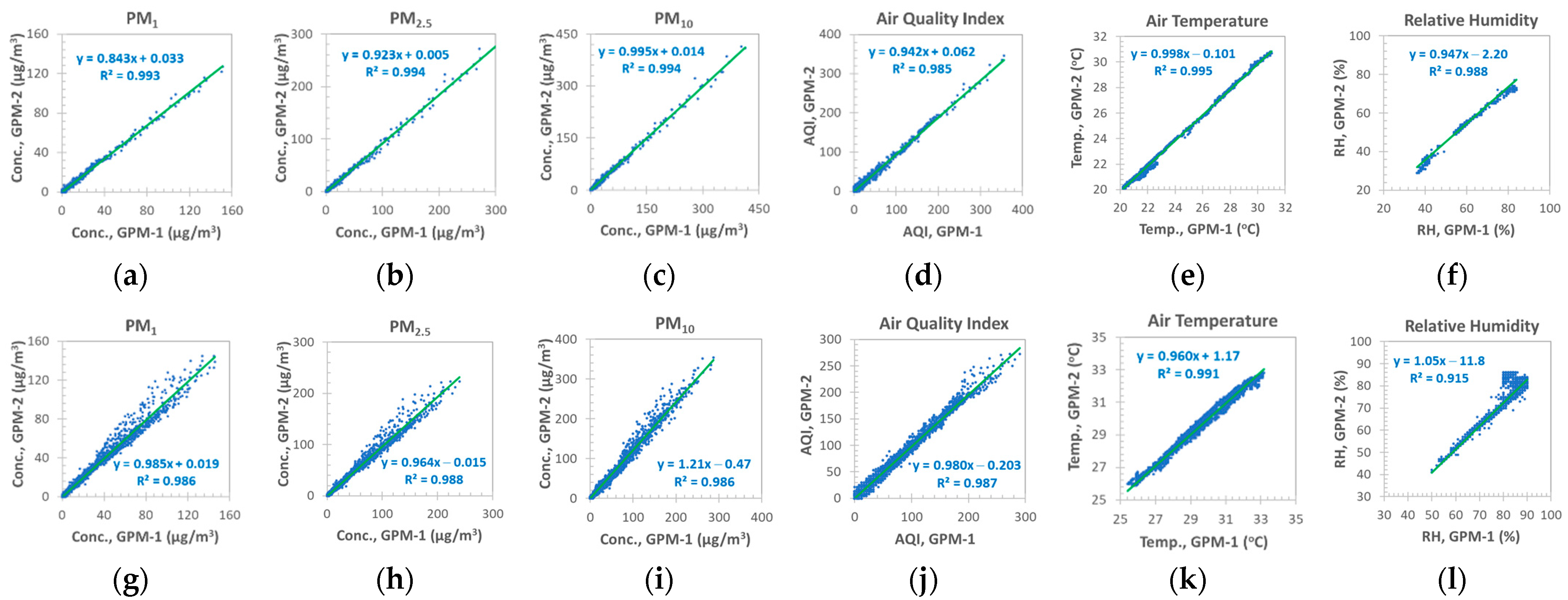
The concentration of PM1, PM2.5, and PM10 observed in the smoke chamber under varying RH with the assistance of GPM sensors (Figure 5a–c) reached as high as 145, 300, and 400 µg/m3, respectively, while AQI peaked at 290 (Figure 5d). It should be noted that the peak mass concentrations of the three PMx species are different (e.g., Figure 5a,c) despite the application of a chemically stable, monodispersed polystyrene DVB for aerosol production. This is likely due to the coagulation of the evolved aerosol, which starts already in the aerosol generator and continues in the transfer tubing towards the smoke chamber. Certainly, this effect is more expressed in the smoke chamber itself, where the aerosol is of higher residence times than in the former units.
As seen for low/medium (Figure 5a–c) and medium/high (Figure 5g–i) RH conditions, the GPM sensors show strong correlations for each PMx range, manifested in high R values (0.993–0.997). In general, the S of the linear fits for PMx approached unity well, ranging between 0.923 and 0.995, except for PM1 under low RH (S = 0.84) (Figure 5a) and for PM10 under high RH (S = 1.21) (Figure 5i). Nevertheless, these close calibration slopes and low intercepts point towards the good intra-model accuracy of the GPMs.
As observed for PMx, similarly sharp linear fitting was attained for AQI (S = 0.94/0.98, R = 0.993/0.995) and Ta (S = 0.94/0.98, R = 0.993/0.995) under any RHs (Figure 5d,e,j,k). On the other hand, a slightly lower correlation of the RH data was obtained under higher RH (R = 0.957) with close to an ideal slope (S = 1.05), but an increased intercept (−11.8%), compared to those observed under low/medium RH (intercept: 2.2%, R = 0.994) (Figure 5f vs. Figure 5l). Interestingly, the RH curve for GPMs starts to “saturate” and shows a higher spread for concurrent RH readings higher than 80%. This finding is not merely unexpected when one recalls the plots for high RH determinations, as reported in Section 3.1. Apparently, monitoring under high RH conditions in the smoke chamber could be characterized by higher uncertainty than those measurements performed in the low/medium RH range.
It is also noticed in Figure 5 that there is a strikingly different evolution of PMx plots towards higher concentrations under low/medium and medium/high RHs. The former curves show homoscedasticity (Figure 5a–c), whereas the latter is rather strongly heteroscedastic (Figure 5g–i), i.e., displaying increasing variance towards higher aerosol concentrations. Similar divergence can be observed for AQI and Ta plots (Figure 5k,l).

BH1 Sensors

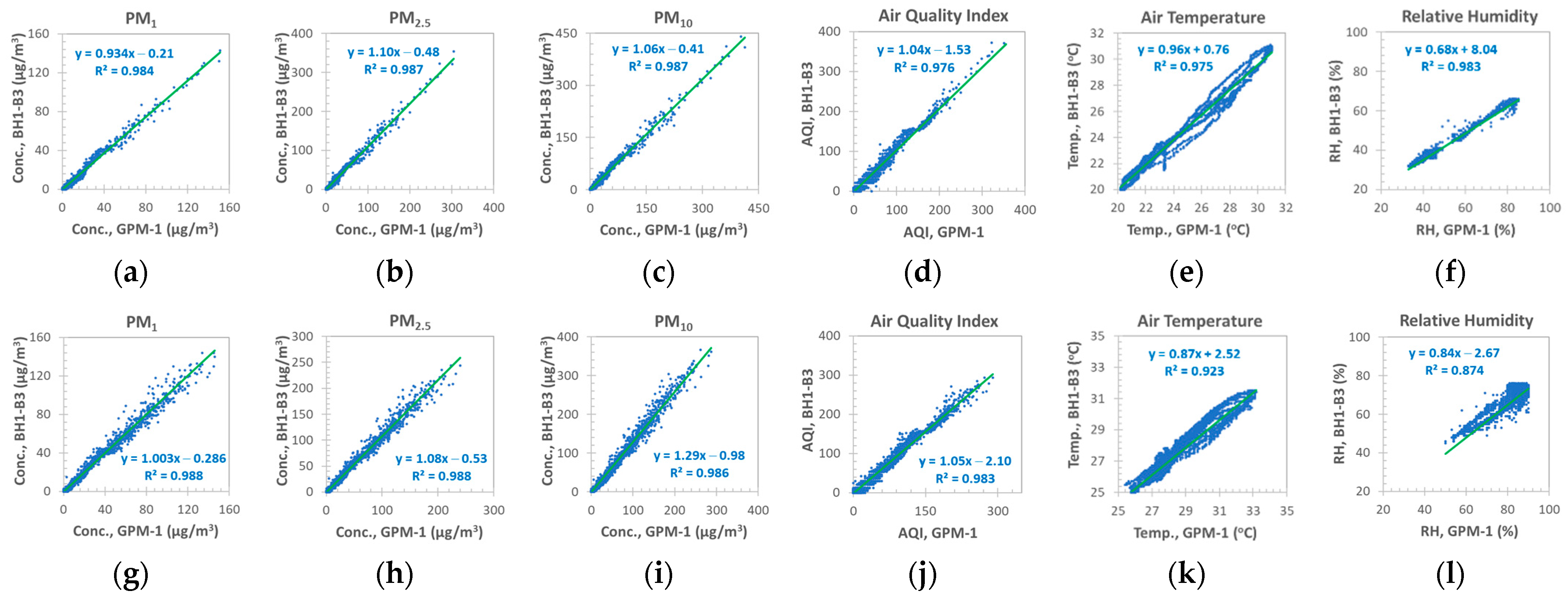
The maximum concentrations of PM1, PM2.5, and PM10 recorded in the smoke chamber with the assistance of BH1-A3 and B3 sensor designs under low/medium RH were as high as 183, 464, and 594 µg/m3, respectively (Figure 6). As it appears, the BH1-A3 and B3 sensors demonstrate strong correlations for each size range of PM, shown with high R values (0.985–0.993). The S of the linear fittings for PM1, PM2.5, and PM10 was close to the unity, i.e., 1.07, 1.13, and 1.04, respectively. On the other hand, the increased intercepts of the fittings (1.6–5.3 µg/m3) indicate an enhanced baseline bias for the model A3 sensor in each PM size range. This result is in accordance with former findings from a field monitoring study conducted with the same type of LCS [17]. The AQIs of A3 and B3 sensors correlated well, too (R ≈ 0.98, S = 0.93), whereas the high intercept of ≈23 points to an increased positive bias of the BH1-A3 sensor, which, nevertheless, is still acceptable for AQ reporting. The concurrent values of Ta and RH show a strong correlation between the two BH1 sensor models (R = 0.979 and 0.994, respectively). Both linear fits are characterized with S of ≈1.06 and low intercepts (−1.5 °C and 0.5%, respectively). Fitting to the AQI data series of the BH1-A3 and B3 sensors also revealed that they followed a slightly S-shaped curvature, an interesting feature that has not been observed for BH1 models in a field study [17].
Under medium/high RH (Figure 7), the BH1-B3 sensors show strong correlations for each PMx, manifested in high R values of the regression fits (0.976–0.985). This is a somewhat lower correlation compared to those observed between sensor models of B3 and A3, which is due most likely to the different RHs applied for the tests. The S of the fitting equations for PM1 and PM2.5 approached unity fairly well, i.e., 0.91 and 1.24, whereas, oddly, a higher value of 1.5 was found for PM10. In general, a higher spread of the data could be observed at PM1, PM2.5, and PM10 concentrations higher than about 50, 70, and 100 µg/m3, respectively. This deviation could be due to the “saturation” under high RH conditions and/or higher inhomogeneity of PM in the smoke chamber, a possible result of internal heating, which causes an upwards convective stream of suspended particulate. In general, low intercepts have been calculated for PM1, PM2.5, and PM10, i.e., 0.25, −0.31, and −0.42 µg/m3, respectively, pointing to a low bias. The AQI data of the B3 sensors also correlated well (R = 0.972, S = 1.18although with a much lower intercept (−2.0) compared to that of the BH1-A3 sensor (Figure 6). The simultaneously recorded data for Ta and RH correlated strongly between the BH1-B3 sensors (R = 0.975 and 0.98, respectively), while S of 0.79 and 1.22, respectively, were obtained with slightly enhanced intercepts, i.e., 3.8 °C, and −6.8%, respectively. These biases are still acceptable for the purpose of environmental monitoring.

3.2.2. Comparison of Sensors of Different Types

GPM versus BH1 Sensors

The fitted PMx data recorded in the smoke chamber with the assistance of GPM and BH1 sensors under various RH conditions are plotted in Figure 8. It appears that the R values of the linear fit for each PM fraction were close to 0.993, which indicates a strong correlation; moreover, it is independent of RH (Figure 8a–c,g–i). The PM1, PM2.5, and PM10 concentrations in the smoke chamber peaked at 150, 354, and 440 µg/m3, respectively (Figure 5a–c).
The S of the linear regression fit for PM1, PM2.5, and PM10 approached the ideal quite well for low/medium RH, i.e., 0.93, 1.1, and 1.06, respectively (Figure 8a–c), whereas for medium/high RH, the S was similar or slightly higher, i.e., 1.00, 1.08, and 1.29, respectively (Figure 8g–i). The intercepts of the fits were low for low/medium RH, i.e., −0.21, −0.48, and −0.41 µg/m3, respectively, while slightly increased bias was observed at high RH, i.e., −0.29, −0.53, and −0.98 µg/m3, respectively. Close fitting was, in general, found for AQI data (R ≈ 0.99, S ≈ 1.04) with negligibly low intercepts (−1.5 and −2.1) at each RH range (Figure 8d,j). A good fit was established for the data series of Ta recorded under low/medium RH (R = 0.987, S = 0.96, intercept: 0.76 °C, see Figure 8e), while for higher RH (Figure 8k) lower correlation and higher bias was found (R = 0.96, S = 0.87, intercept: 2.5 °C). Although the RH data strongly correlated under low/medium RH (R = 0.966), the fitting deviated from the ideal (S = 0.68) with a quite high intercept (8%), pointing towards systematic errors (Figure 8f). Interestingly, a better fit was acquired for higher RH (R = 0.935, S = 0.84), with a lower intercept (−2.7%, Figure 8l) than the former (Figure 8f). Like the above observations (Section “GPM Sensors”), homoscedastic graphs were found under low/medium RH, whereas the calibration plots become heteroscedastic at medium/high RHs.

GPM versus GRIMM Monitor

The PMx and AQI data series obtained with the GPM and GRIMM sensors (Figure 9) are characterized by strong correlations (R ≈ 0.984–0.988). The S of the regression fits for PM2.5 approached the ideal accurately (1.03), whereas lower and higher values for PM1 and PM10 were observed, i.e., 0.703 and 1.22, respectively. These data show that the GPM sensor has lower detection capability towards accurately predicting fine and coarse (PM10–2.5) aerosol fractions, due likely to the much lower bin number of the PMS5003 sampler, compared to the GRIMM sensor. The intercepts of the fitting equations were negligibly low for each PMx species and AQI, ranging from 0.2 to 0.44 µg/m3 and 0.61, respectively. Interestingly, the results on the overestimate of PM10 readings are not in line with the findings in Refs. [13,14,26], reporting underestimates for coarse aerosol when applying LCSs equipped with PMS5003 sensors.

BH1 versus GRIMM Monitor

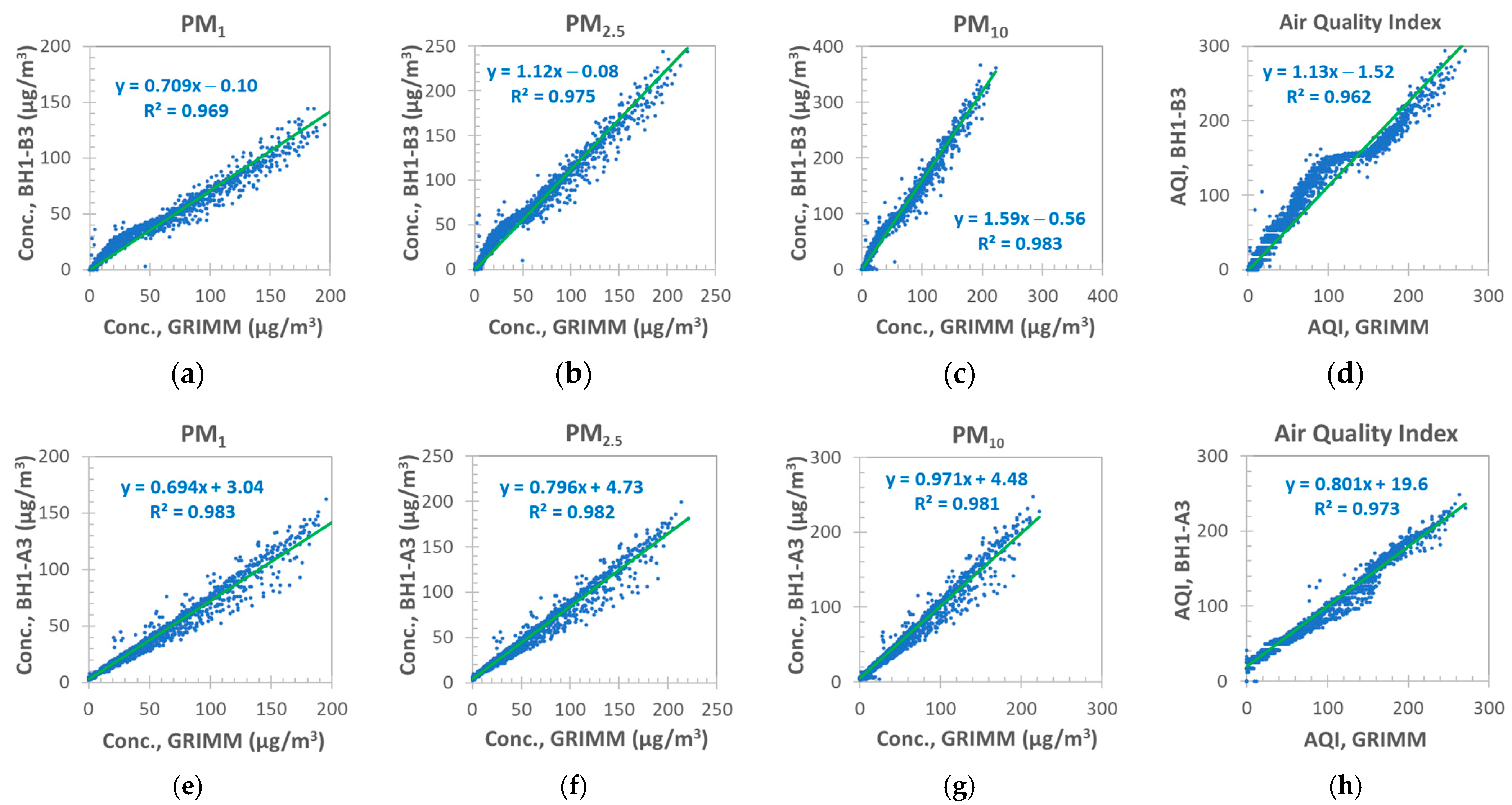
Similar observations to those attained for GPM and GRIMM were made when comparing BH1 sensors (designs A3 and B3) with the GRIMM reference monitor under medium/high RH conditions (Figure 10). The B3 sensor approached PM2.5 and AQI accurately (S ≈ 1.12, R ≈ 0.98). A very low bias was found for PMx, ranging between −0.08 and −0.56 µg/m3, and for AQI too (−1.52). On the other hand, slightly higher PM10 readings were observed with BH1-B3 (S = 1.59), compared to GPM and GRIMM, which is somewhat higher than well accepted for environmental monitoring, i.e., the S value should be a maximum of 1.35 [46]. Accordingly, the PM10 data recorded with the BH1-B3 requires a definite mathematical correction and calibration in the laboratory and on the field as well.
For the BH1-A3 model and the GRIMM monitor under medium/high RHs, less steep slopes of PM1, PM2.5, and PM10 and AQI were obtained with S data of 0.694, 0.796, 0.97, and 0.80, respectively, which are still acceptable for AQ reporting. On the other hand, the intercepts of the fits for PM1, PM2.5, and PM10 are fairly enhanced, i.e., 3.0, 4.7, and 4.5 µg/m3, respectively, pointing to biased measurements with this sensor at low aerosol levels. The LOD values calculated for this sensor type under high RH conditions support this affirmation (see Section 3.3.2) and are in quite good agreement with the corresponding PMx bias. Nonetheless, these calibration curves invoke errors, which is still acceptable for AQ reporting, as one recalls the US EPA recommendations [46].

3.3. Analytical Performance of the Sensors

3.3.1. Error of the LCSs for Ambient Microclimatic Parameters

The error indicator metrics of the GPM and BOHU LCSs, evaluated for Ta, are presented in Table 1. As can be seen, under low RH, the RMSE for Ta ranged from 0.7 to 1.9 °C (average: 1.2 °C, median: 1.0 °C) for GPM and BH1 sensors, while MNE ranged from 2.4 to 6.7% (average: 3.9%, median: 3.3%). For medium RH, the RMSE for Ta was in the range of 0.8 to 1.7 °C (average: 1.1 °C, median: 1.0 °C) for the two types of LCSs, whereas the MNE increased, lying in the range of 2.4–7.7% (average: 4.7%, median: 4.4%). Under high RH in the smoke chamber, the RMSE for Ta was in the range of 0.8–2.2 °C (average: 1.6 °C, median: 1.7 °C), whereas MNE was between 2.5 and 7.5% (average: 5.3%, median: 5.7%). These data all show that, in general, the bias of the Ta readings with the study LCSs increases slightly in the medium, especially in the high RH range, compared to low RH conditions. The MNB values were similar or lower compared to MNE for each LCS in any studied RH range.
As appears in Table 2, the LCSs (GPM and BOHU) for RH monitoring have shown larger errors than those calculated for Ta. Under low RH conditions, the RMSE was fairly low, i.e., it ranged from 1.2 to 5.4% (average: 3.5%, median: 3.7%), while the MNE was high, ranging between 3.2% and 15.5% (average: 9.8% (rel.), median: 10.4% (rel.)) for GPM and BOHU sensors. Under medium RH conditions, higher RMSE was experienced between 4.4% and 9.7% (average: 7.3%, median: 7.6%), while MNE ranged from 5.6 to 12.5% (rel.) (average: 15.6% (rel.), median: 15.1% (rel.)). For high RHs, the RMSE increased significantly, ranging between 9.7 and 21.6% (average: 15.2%, median: 14.6%), whereas MNE ranged from 9.5. to 22.8 (average: 15.6% (rel.), median: 15.1% (rel.)) for the two sensor designs. The MNB values were found to be similar or slightly lower compared to MNE data for each LCS over any studied RH range. It can also be seen that the bias in several cases is negative, corresponding to an underestimation of the true value by the use of the LCSs. Overall, the pattern is obvious for RH measurements: the higher the RH, the higher the bias of the readings obtained from LCSs. Nevertheless, both error indicators showed an aptly low level (<30%) as recommended for LCS testing by US EPA [46].

3.3.2. Performance of LCSs for Size-Segregated Aerosol

The error indicator metrics were evaluated for various PMx species besides the concurrent Ta and RH data, registered every 1 min with the assistance of the studied LCSs (Table 3). As can be seen, under low/medium RH, the GPM-1 and GPM-2 sensors showed quite low RMSE for PM1, PM2.5, and PM10, i.e., 3.8, 6.5, and 15 µg/m3, respectively, whereas increased bias was experienced under high RH conditions, e.g., 5.7, 8.2, and 26 µg/m3, respectively. On the other hand, under low/medium RH, the MNE values of PM1, PM2.5, and PM10 were 7.0, 9.1, and 11.7%, while similar or higher MNEs of 8.5, 8.6, and 17.2%, respectively, were experienced for high RHs. Interestingly, for Ta and RH, the RMSE and the MNE values were of a similar extent under medium and high RH conditions for both GPMs. Under medium RH conditions, the MNB shows a different pattern for PM1, PM2.5, and PM10, i.e., −4.3, −6.4, and 9.0%, respectively, whereas at high RH, its value changed differently for the three PMx species, i.e., 4.6, 0.9, and 19.4%, respectively. These data indicate the negative bias of the LCSs for low/medium sized PM under low/medium RH, whereas the bias is positive for coarser aerosol, manifested in PM10 at high RHs.
Under medium RHs, the GPM and BH1-A3 LCSs demonstrated somewhat higher RMSE as compared to that experienced between the two GPM sensors, except for PM10 of a similar extent. The RMSE for PM1, PM2.5, and PM10 was 7.1, 11.3, and 13.8 µg/m3, respectively, while an increased bias was obtained at high RHs, i.e., 7.8, 18, and 21 µg/m3, respectively. Similarly, the MNE increased compared to those found between the GPMs. Under low/medium RHs, the MNE for PM1, PM2.5, and PM10 was high, i.e., 21, 33, and 36%, while similar or higher values of 22, 41, and 46%, respectively, were experienced for high RH conditions. At low/medium RH, the MNB data showed an increasing pattern from PM1, PM2.5, to PM10 with values of −7.7, −23, and −24%, respectively, whereas at high RH, it increased to −12, −27, and −29%, respectively. For Ta and RH, the RMSE and the MNE between BH1-A3 and any of the GMPs were of similar extent, irrespective of RH in the smoke chamber, except for GPM-1 that was a five-fold higher value (14%).
The error indicators evaluated for various PMx species, registered every 1 min with the study LCSs against the reference sensor, are listed in Table 4. As can be seen, under medium RH conditions, the GPM-1 and GPM-2 sensors showed quite similar RMSE for PM1 and PM2.5, i.e., about 20 and 10 µg/m3, respectively, whereas somewhat increased bias was experienced for PM10 of GPM-2 (30 µg/m3). A similar pattern was observed for MNE of PM1 and PM2.5, i.e., about 24% and 42%, respectively, whereas an increased value was experienced for PM10 of GPM-2 (64%). Under high RH conditions, the RMSE increased slightly for PM1 and PM2.5, whereas a higher increment of PM10 was observed. This effect is likely due to the higher rate of particle growth under increasing RHs, which brings more uncertainty in the measurement of coarse aerosol [49]. The MNB was quite high in the case of GPM sensors, apart from PM1 (−2.8/−8.5%), and more or less acceptable for PM2.5 (41/33%) but outstandingly high for PM10 (65/57%). These findings point to the lesser usability of the GPM sensor for coarse aerosol quantitation.
Under medium RH, the BH1-A3 sensor featured similar or lower RMSE as compared to those found for GPM sensors against the reference monitor. For instance, the RMSE for PM1, PM2.5, and PM10 was 14, 7.4, and 7.8 µg/m3, respectively, whereas its increase was observed at high RH, i.e., 22, 16, and 9.3 µg/m3, respectively. The MNE formed a similar pattern to the RMSE. Under medium RH, the MNE of PM1, PM2.5, and PM10 for the BH1-A3 sensor was found to be 17, 13, and 20%, respectively, whereas under high RHs, it was 25, 19, and 17%, respectively. Interestingly, for BH1-A3 sensors, the RMSE and the MNE values develop a decreasing trend from PM1 towards higher PMx ranges, which is the opposite order experienced for the GPMs. Similar patterns of RMSE and MNE were observed for the BH1-B3 sensor (Table 4). Under low/medium RH conditions, the MNB displayed a varying bias for PM1, PM2.5, and PM10 with −15, 5, and 20%, respectively, whereas decreased values were found for high RH conditions.
The LOD and the LOQ data under low/medium and high RH conditions are presented in Table 5. As can be seen, at low-to-high RH, the LODs of each PMx fraction for the GPM and the BH1-B3 sensors are advantageously low (1.5 µg/m3) compared to those calculated for the BH1-A3 (3.5–4.5 µg/m3). This is likely due to the higher background noise of the latter design, manifested in enhanced readings (2–3 µg/m3) in the otherwise clean air. These LOD data are in line with those observed for GPM and BH1-A3 in field campaigns, although the latter value was slightly higher due to the higher background PM levels [17].
On the other hand, for the GRIMM monitor, the LOD as low as 0.25 µg/m3 was experienced due to the higher sensor sensitivity towards finer PM fractions, which arises from the enhanced detection capability for lower aerosol masses, compared to GPM and BH1 sensors. In general, under low/medium RHs, lower LOD values of PMx for the BH1-A3 sensors were attained, whereas the rest of the study sensors experienced the same LODs at various RHs.

4. Discussion

The literature reports on several kinds of LCSs based on PMS5003, as noticed above, and a couple of AQ networks, including PurpleAir [22,23,24,25,26] and Clarity [13]. Moreover, this sensor has been applied in several geospatial and exposure studies, for instance, in Refs. [50,51]. A couple of studies suggest that the readings for PM1 and PM2.5 of this LCS are in good correlation with those measured against reference methods, but its low performance was found for coarse aerosol, e.g., PM10–2.5 [8,14,15,50].
In a former field monitoring study [17], the GPM and the BH1-A3 sensors provided similar linearity for indoor and outdoor aerosols. But a relatively short PM mass concentration range could be covered and assessed for calibration, i.e., up to about 130 µg/m3 for PM10. Moreover, the studied LCSs could be measured against a less sharp OPC sensor, which could only assess PM2.5 levels but not give information on accuracies towards fine and coarse aerosol fractions. In this investigation, it was shown that the studied LCSs can be calibrated and tested with monodispersed spherical latex aerosol introduced into a laboratory smoke chamber for a much higher concentration range of the aerosol under controlled slow heating and/or varying RH conditions. By using an aerosol generator, as high PM1, PM2.5, and PM10 levels as about 150, 350, and 450 µg/m3, respectively, were reached in the smoke chamber. This is already about three times higher PMx concentration than those obtained in the former field study, with similar types of LCSs [17]. In general, linear relationships were established between the concurrently registered data with the various OPCs regarding intra- and inter-model accuracy.
For this investigation, some LCSs, such as Geekcreit PMx, built on a PMS5003 sampler, and BOHU BH1 (models A3 and B3) monitors (built with a Pando G7 OPC) were compared with a laboratory-grade sensor, GRIMM 1.109 used as a reference monitor. The results have clearly shown that the accuracy of the readings for PM1, PM2.5, and PM10 with the different and the same types of LCSs was acceptable, corresponding to those observed by means of the reference, research-grade sensor. The GPM sensors are based on PMS5003 OPC, which is characterized by low detection efficacy for coarse PM [13,14,26]. This would introduce some bias into the determination of the coarse fraction, i.e., PM10–2.5, manifested in the underestimate of PM10 levels. On the other hand, in this study, an overestimate was observed for PM10 by the PMS-based LCSs, indicating the coagulation of particulates and a positive bias of higher RH on the PM10 determinations.
Controlled slow heating (0.2 °C/min) of the smoke chamber was advantageous for calibration/checking of the Ta sensors of the monitors against an industrial-grade, analog thermometer, whereas Ta data observed during the cooling stage of the smoke chamber was rather hampered by higher measurement bias.
The RH sensors of the LCSs were assessed with the application of slow evaporation of boiled/hot water in the smoke chamber. With this simple procedure, even the medium and high RH ranges could be covered for calibration. Nevertheless, the high RH ranges are less accurately approached and had the drawback of lower detection efficacy, as can be seen from the analytical performance/error indicator metrics (RMSE, MNE, MNB, LOD, and LOQ).

5. Conclusions

In this study, various laboratory conditions inside a smoke chamber were adjusted for the calibration of low-cost air quality devices, i.e., Geekcreit and BOHU BH1 models A3 and B3, each based on the OPC principle for PMx components. Microclimatic variables such as air temperature and relative humidity were also monitored. It was demonstrated that the LCSs provided generally accurate readings for PM2.5, irrespective of the air temperature and relative humidity changes in the smoke chamber. On the other hand, the PM1 and PM10 readings of the LCSs (irrespective of either with PMS5003 or Pando G7 sampler) were slightly lower and higher, respectively, compared to those recorded with the research-grade air monitor. This is likely due to the lower detection efficacy of the fine and coarse fraction of ambient aerosol with the assistance of low-cost OPCs possessing a low number of bins. Moreover, at high RH, the calibration plots showed heteroscedasticity (about 10–20% increase in bias) towards higher PMx concentrations, which was also observed for AQI, Ta, and RH calibration curves.
For temperature calibration, it appears that the low RH in the smoke chamber provided more reproducible conditions in terms of the lowest measurement bias for LCSs as recorded against a reference-grade analog thermometer. The relative humidity measurements with the LCSs performed against an industrially calibrated RH meter provided accurate readings at the low and medium RH range, but high RHs caused increased bias. Although the experimental arrangement with the smoke chamber provided relatively reliable values for PMx and microclimatic parameters, the accuracy of the data could be improved, for instance, with the application of lower volumes of the aerosol chamber, lower heating rates, and more sharply controlled RH conditions, e.g., by means of those reported in Ref. [41].

Author Contributions

Conceptualization, L.B. and A.N.; methodology, L.B. and A.N.; validation, L.B.; formal analysis, L.B.; investigation, L.B. and A.N.; resources, L.B. and A.N.; data curation, L.B.; writing—original draft preparation, L.B.; writing—review and editing, L.B. and A.N.; visualization, L.B.; supervision, L.B. and A.N.; project administration, L.B. and A.N.; funding acquisition, L.B. and A.N. All authors have read and agreed to the published version of the manuscript.

Funding

This research was partially supported by the Hungarian National Research Development and Innovation Fund under grant No. TKP2021-NVA-04.

Institutional Review Board Statement

Not applicable.

Informed Consent Statement

Not applicable.

Data Availability Statement

The data are not publicly available due to file size limitations. The research data presented in this study are available on request from the corresponding author.

Acknowledgments

The authors thank the support provided by their research institution (Wigner RCP) for providing funds for the analytical spectroscopic and aerosol research laboratories.

Conflicts of Interest

The authors declare no conflicts of interest.

References

  1. Dockery, D.W.; Speizer, F.E.; Stram, D.O.; Ware, J.H.; Spengler, J.D.; Ferris, B.G., Jr. Effects of inhalable particles on respiratory health of children. Am. Rev. Respir. Dis. 1989, 139, 587–594. [Google Scholar] [CrossRef]
  2. Camuffo, D. Microclimate for Cultural Heritage: Measurement, Risk Assessment, Conservation, Restoration, and Maintenance of Indoor and Outdoor Monuments, 3rd ed.; Elsevier B.V.: Amsterdam, The Netherlands, 2019. [Google Scholar]
  3. Spolnik, Z.; Bencs, L.; Worobiec, A.; Kontozova, V.; Van Grieken, R. Application of EDXRF and thin window EPMA for the investigation of the influence of hot air heating on the generation and deposition of particulate matter. Microchim. Acta 2005, 149, 79–85. [Google Scholar] [CrossRef]
  4. Anaf, W.; Bencs, L.; Van Grieken, R.; De Wael, K.; Janssens, K. Indoor particulate matter in four Belgian heritage sites: Case studies on the deposition of dark-colored and hygroscopic particles. Sci. Total Environ. 2015, 506–507, 361–368. [Google Scholar] [CrossRef]
  5. IPCC. Climate Change 2021: The Physical Science Basis, Sixth Assessment Report; Cambridge University Press: Cambridge, UK, 2021. [Google Scholar]
  6. Kelly, K.E.; Whitaker, J.; Petty, A.; Widmer, C.; Dybwad, A.; Sleeth, D.; Martin, R.; Butterfield, A. Ambient and laboratory evaluation of a low-cost particulate matter sensor. Environ. Pollut. 2017, 221, 491–500. [Google Scholar] [CrossRef]
  7. Zamora, M.L.; Xiong, F.Z.L.; Gentner, D.; Kerkez, B.; Kohrman-Glaser, J.; Koehler, K. Field and Laboratory Evaluations of the Low-Cost Plantower Particulate Matter Sensor. Environ. Sci. Technol. 2019, 53, 838–849. [Google Scholar] [CrossRef]
  8. Sayahi, T.; Butterfield, A.; Kelly, K.E. Long-term field evaluation of the Plantower PMS low-cost particulate matter sensors. Environ. Pollut. 2019, 245, 932–940. [Google Scholar] [CrossRef] [PubMed]
  9. Sayahi, T.; Kaufman, D.; Becnel, T.; Kaur, K.; Butterfield, A.E.; Collingwood, S.; Zhang, Y.; Gaillardon, P.E.; Kelly, K.E. Development of a calibration chamber to evaluate the performance of low-cost particulate matter sensors. Environ. Pollut. 2019, 255, 113131. [Google Scholar] [CrossRef] [PubMed]
  10. Zusman, M.; Schumacher, C.S.; Gassett, A.J.; Spalt, E.W.; Austin, E.; Larson, T.V.; Carvlin, G.; Seto, E.; Kaufman, J.D.; Sheppard, L. Calibration of low-cost particulate matter sensors: Model development for a multi-city epidemiological study. Environ. Int. 2020, 134, 105329. [Google Scholar] [CrossRef]
  11. Hedge, S.; Min, K.T.; Moore, J.; Lundrigan, P.; Patwari, N.; Collingwood, S.; Balch, A.; Kelly, K.E. Indoor Household Particulate Matter Measurements Using a Network of Low-cost Sensors. Aerosol Air Qual. Res. 2020, 20, 381–394. [Google Scholar]
  12. Peck, A.; Handy, R.G.; Sleeth, D.K.; Schaefer, C.; Zhang, Y.; Pahler, L.F.; Ramsay, J.; Collingwook, S.C. Aerosol Measurement Degradation in Low-Cost Particle Sensors Using Laboratory Calibration and Field Validation. Toxics 2023, 11, 56. [Google Scholar] [CrossRef] [PubMed]
  13. Kaur, K.; Kelly, K.E. Laboratory evaluation of the Alphasense OPC-N3, and the Plantower PMS5003 and PMS6003 sensors. J. Aerosol Sci. 2023, 171, 106181. [Google Scholar] [CrossRef]
  14. Kuula, J.; Mäkelä, T.; Aurela, M.; Teinilä, K.; Varjonen, S.; González, O.; Timonen, H. Laboratory evaluation of particle-size selectivity of optical low-cost particulate matter sensors. Atmos. Meas. Tech. 2020, 13, 2413–2423. [Google Scholar] [CrossRef]
  15. Vogt, M.; Schneider, P.; Castell, N.; Hamer, P. Assessment of Low-Cost Particulate Matter Sensor Systems against Optical and Gravimetric Methods in a Field Co-Location in Norway. Atmosphere 2021, 12, 961. [Google Scholar] [CrossRef]
  16. Hong, G.W.; Le, T.C.; Tu, J.W.; Wang, C.E.; Chang, S.C.; Yu, Y.; Lin, G.Y.; Aggarwal, S.G.; Tsai, C.J. Long-term evaluation and calibration of three types of low-cost PM2.5 sensors at different air quality monitoring stations. J. Aerosol Sci. 2021, 157, 105829. [Google Scholar] [CrossRef]
  17. Bencs, L.; Plósz, B.; Mmari, A.G.; Szoboszlai, N. Comparative Study on the Use of Some Low-Cost Optical Particulate Sensors for Rapid Assessment of Local Air Quality Changes. Atmosphere 2022, 13, 1218. [Google Scholar] [CrossRef]
  18. Badura, M.; Sowka, I.; Szymanski, P.; Batog, P. Assessing the usefulness of dense sensor network for PM2.5 monitoring on an academic campus area. Sci. Total Environ. 2020, 722, 137867. [Google Scholar] [CrossRef]
  19. Jiang, Y.X.; Zhu, X.L.; Chen, C.; Ge, Y.H.; Wang, W.D.; Zhao, Z.H.; Cai, J.; Kan, H.D. On-field test and data calibration of a low-cost sensor for fine particles exposure assessment. Ecotoxicol. Environ. Saf. 2021, 211, 111958. [Google Scholar] [CrossRef]
  20. Huang, C.H.; He, J.Y.; Austin, E.; Seto, E.; Novosselov, I. Assessing the value of complex refractive index and particle density for calibration of low-cost particle matter sensor for size-resolved particle count and PM2.5 measurements. PLoS ONE 2021, 16, e0259745. [Google Scholar] [CrossRef]
  21. Cowell, N.; Chapman, L.; Bloss, W.; Pope, F. Field Calibration and Evaluation of an Internet-of-Things-Based Particulate Matter Sensor. Front. Environ. Sci. 2022, 9, 798485. [Google Scholar] [CrossRef]
  22. Ouimette, J.R.; Malm, W.C.; Schichtel, B.A.; Shridan, P.J.; Andrews, E.; Ogren, J.A.; Arnott, W.P. Evaluating the PurpleAir monitor as an aerosol light scattering instrument. Atmos. Meas. Tech. 2022, 15, 655–676. [Google Scholar] [CrossRef]
  23. Wallace, L.; Bi, J.Z.; Ott, W.R.; Sarnat, J.; Liu, Y. Calibration of low-cost PurpleAir outdoor monitors using an improved method of calculating PM2.5. Atmos. Environ. 2021, 256, 118432. [Google Scholar] [CrossRef]
  24. Wallace, L. Intercomparison of PurpleAir Sensor Performance over Three Years Indoors and Outdoors at a Home: Bias, Precision, and Limit of Detection Using an Improved Algorithm for Calculating PM2.5. Sensors 2022, 22, 2755. [Google Scholar] [CrossRef]
  25. Park, S.-J.; Lee, S.H.; Yeo, M.S.; Rim, D.H. Field and laboratory evaluation of PurpleAir low-cost aerosol sensors in monitoring indoor airborne particles. Build. Environ. 2023, 234, 110127. [Google Scholar] [CrossRef]
  26. Tryner, J.; L’Organge, C.; Mahaffy, J.; Miller-Lionberg, D.; Hofstetter, C.; Wilson, A.; Volckens, J. Laboratory evaluation of low-cost PurpleAir PM monitors and in-field correction using co-located portable filter samplers. Atmos. Environ. 2020, 220, 117067. [Google Scholar] [CrossRef]
  27. Jayaratne, R.; Liu, X.T.; Thai, P.; Dunbabin, M.; Morawska, L. The influence of humidity on the performance of a low-cost air particle mass sensor and the effect of atmospheric fog. Atmos. Meas. Tech. 2018, 11, 4883–4890. [Google Scholar] [CrossRef]
  28. Wahlborg, D.; Björling, M.; Mattsson, M. Evaluation of field calibration methods and performance of AQMesh, a low-cost air quality monitor. Environ. Monit. Assess. 2021, 193, 251. [Google Scholar] [CrossRef] [PubMed]
  29. Castell, N.; Dauge, F.R.; Schneider, P.; Vogt, M.; Lerner, U.; Fishbain, B.; Broday, D.; Bartonova, A. Can commercial low-cost sensor platforms contribute to air quality monitoring and exposure estimates? Environ. Int. 2017, 99, 293–302. [Google Scholar] [CrossRef] [PubMed]
  30. Thorpe, A.; Walsh, P.T. Comparison of Portable, Real-Time Dust Monitors Sampling Actively, with Size-Selective Adaptors, and Passively. Ann. Occup. Hyg. 2007, 51, 679–691. [Google Scholar] [PubMed]
  31. Salimifard, P.; Rim, D.; Freihaut, J.D. Evaluation of low-cost optical particle counters of monitoring individual indoor aerosol sources. Aerosol Sci. Technol. 2020, 54, 217–231. [Google Scholar] [CrossRef]
  32. Semple, S.; Apsley, A.; MacCalman, L. An inexpensive particle monitor for smoker behaviour modification in homes. Tob. Control 2013, 11, 295–298. [Google Scholar] [CrossRef]
  33. Markowich, K.M.; Chiliński, M.T. Evaluation of two low-cost optical particle counters for the measurement of ambient aerosol scattering coefficient and Ångström exponent. Sensors 2020, 20, 2617. [Google Scholar] [CrossRef] [PubMed]
  34. Wang, Y.; Li, J.Y.; Jing, H.; Zhang, Q.; Jiang, J.K.; Biswas, P. Laboratory evaluation and calibration of three low-cost particle sensors for particulate matter measurement. Aerosol Sci. Technol. 2015, 49, 1063–1077. [Google Scholar] [CrossRef]
  35. Crilley, L.R.; Shaw, M.; Pound, R.; Kramer, L.J.; Price, R.; Young, S.; Lewis, A.C.; Pope, F.D. Evaluation of a low-cost optical particle counter (Alphasense OPC-N2) for ambient air monitoring. Atmos. Meas. Tech. 2018, 11, 709–720. [Google Scholar] [CrossRef]
  36. Crnosija, N.; Zamora, M.L.; Rule, A.M.; Payne-Sturges, D. Laboratory Chamber Evaluation of Flow Air Quality Sensor PM2.5 and PM10 Measurements. Int. J. Environ. Res. Public Health 2022, 19, 7340. [Google Scholar] [CrossRef] [PubMed]
  37. Amoh, N.A.; Xu, G.; Kumar, A.R.; Wang, Y. Calibration of low-cost particulate matter sensors for coal dust monitoring. Sci. Total Environ. 2023, 859, 160336. [Google Scholar] [CrossRef]
  38. Jayaratne, R.; Liu, X.T.; Ahn, K.-H.; Asumandu-Sakyi, A.; Fisher, G.; Gao, J.; Mabon, A.; Mazaheri, M.; Mullins, B.; Nyaku, M.; et al. Low-cost PM2.5 Sensors: An Assessment of their Suitability for Various Applications. Aerosol Air Qual. Res. 2020, 20, 520–532. [Google Scholar] [CrossRef]
  39. Sousan, S.; Regmi, S.; Park, Y.M. Laboratory Evaluation of Low-Cost Optical Particle Counters for Environmental and Occupational Exposures. Sensors 2021, 21, 4146. [Google Scholar] [CrossRef]
  40. Si, M.X.; Xiong, Y.; Du, S.; Du, K. Evaluation and calibration of a low-cost particle sensor in ambient conditions using machine-learning methods. Atmos. Meas. Tech. 2020, 13, 1693–1707. [Google Scholar] [CrossRef]
  41. Rivero, R.A.G.; Hernández, L.E.M.; Schalm, O.; Rodríguez, E.H.; Sánchez, D.A.; Pérez, M.C.M.; Caraballo, V.N.; Jacobs, W.; Laguardia, A.M. A Low-Cost Calibration Method for Temperature, Relative Humidity, and Carbon Dioxide Sensors Used in Air Quality Monitoring Systems. Atmosphere 2023, 14, 191. [Google Scholar] [CrossRef]
  42. Alfano, B.; Barretta, L.; Del Giudice, A.; De Vito, S.; Di Francia, G.; Esposito, E.; Formisano, F.; Massera, E.; Miglietta, M.L.; Polichetti, T. A review of low-cost particulate matter sensors from the developers’ perspectives. Sensors 2020, 20, 6819. [Google Scholar] [CrossRef]
  43. Giordano, M.R.; Malings, C.; Pandis, S.N.; Presto, A.A.; McNeill, V.F.; Westervelt, D.M.; Beekmann, M.; Subramanian, R. From low-cost sensors to high-quality data: A summary of challenges and best practices for effectively calibrating low-cost particulate matter sensors. J. Aerosol Sci. 2021, 158, 105833. [Google Scholar] [CrossRef]
  44. Rai, A.C.; Kumar, P.; Pilla, F.; Skouloudis, A.N.; Di Sabatino, S.; Ratti, C.; Yasar, A.; Rickerby, D. End-user perspective of low-cost sensors for outdoor air pollution monitoring. Sci. Total Environ. 2017, 607, 691–705. [Google Scholar] [CrossRef] [PubMed]
  45. Yuval; Molho, H.M.; Zivan, O.; Broday, D.M.; Raz, R. Application of a sensor network of low cost optical particle counters for assessing the impact of quarry emissions on its vicinity. Atmos. Environ. 2019, 211, 29–37. [Google Scholar] [CrossRef]
  46. US EPA (United States Environmental Protection Agency); Duvall, R.M.; Clements, A.L.; Hagler, G.; Kamal, A.; Kilaru, V.; Goodman, L.; Frederick, S.; Barkjohn, K.K.; VonWald, I.; et al. Performance Testing Protocols, Metrics, and Target Values for Fine Particulate Matter Air Sensors. EPA/600/R-20/280. Available online: https://www.epa.gov/ (accessed on 25 January 2024).
  47. IUPAC; Inczédy, J.; Lengyel, T.; Ure, A.M.; Gelencsér, A.; Hulanicki, A. (Eds.) Compendium of Analytical Nomenclature, 3rd ed.; Blackwell: Oxford, UK, 1998. [Google Scholar]
  48. European Commission. Directive 2008/50/EC of the European Parliament and the Council of 21 May 2008 on Ambient Air Quality and Cleaner Air for Europe. Off. J. Eur. Union 2008. Available online: https://eur-lex.europa.eu/legal-content/EN/TXT/?uri=OJ:L:2008:152:TOC (accessed on 25 January 2024).
  49. Won, W.S.; Oh, R.; Lee, W.; Ku, S.K.; Su, P.C.; Yoon, Y.J. Hygroscopic properties of particulate matter and effects of their interactions with weather on visibility. Sci. Rep. 2021, 11, 16401. [Google Scholar] [CrossRef]
  50. Bi, J.; Wildani, A.; Chang, H.H.; Liu, Y. Incorporating low-cost sensor measurements into high-resolution PM2.5 modeling at a large spatial scale. Environ. Sci. Technol. 2020, 54, 2152–2162. [Google Scholar] [CrossRef]
  51. Kelly, K.E.; Xing, W.W.; Sayahi, T.; Mitchell, L.; Becnel, T.; Gaillardon, P.-E.; Meyer, M.; Whitaker, R.T. Community-based measurements reveal unseen differences during air pollution episodes. Environ. Sci. Technol. 2021, 55, 120–128. [Google Scholar] [CrossRef]
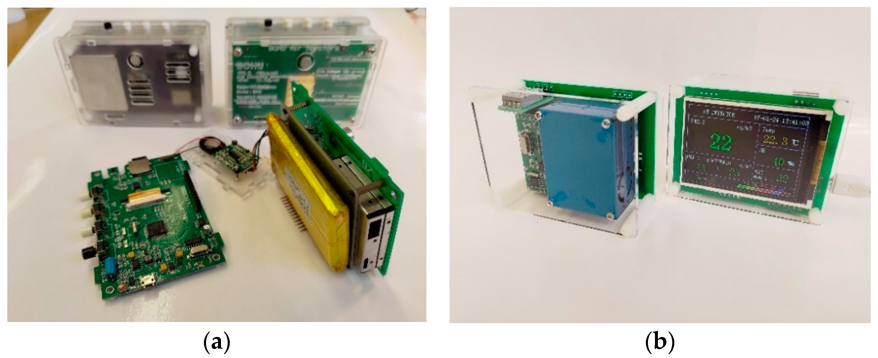
Figure 1. Pictures of the study LCSs: (a) back panels of BH1-B3 and BH1-A3 (background), dismantled A3 sensor: front panel/micro PC board with LCD display (left), and the Pando G7 sampler/battery (grey/yellow units at the right), (b) front and back panel view of the GPM: PMS5003 sampler (blue module), Ta/RH sensor (grey module at the top), and interface/micro-PC board (left).
Atmosphere 15 00304 g001
Figure 2. The smoke chamber with the installed aerosol sensors and microclimatic measurement apparatus (left side in the background: GRIMM OPC; middle: BH1-A3/B3 sensors; right side: GPM sensors and Testo).
Atmosphere 15 00304 g002
Figure 3. Air temperature recorded in the smoke chamber with LCSs, plotted against a reference mercury thermometer under (a) low, (b) medium, and (c) high RH (the color of each equation corresponds to that of the data label/marker).
Atmosphere 15 00304 g003
Figure 4. Relative humidity recorded in the smoke chamber with various LCSs plotted against a reference sensor (Testo) under (a) low, (b) medium, and (c) high RH (the color of each equation corresponds to that of the data label/marker).
Atmosphere 15 00304 g004
Figure 5. Correlation between monitoring data (n = 25,940) registered in the smoke chamber under low/medium RH (upper row) and medium/high RH (lower row) with two GPM sensors; PM1 (a,g), PM2.5 (b,h), PM10 (c,i), AQI (d,j), Ta (e,k), and RH (f,l).
Atmosphere 15 00304 g005
Figure 6. Correlation between monitoring data (n = 25,110) registered with BH1 sensors (models A3 vs. B3) under low/medium RH; PM1 (a), PM2.5 (b), PM10 (c), AQI (d), Ta (e), and RH (f).
Atmosphere 15 00304 g006
Figure 7. Correlation between monitoring data (n = 25,740) registered with BH1-B3 sensors under medium/high RH; PM1 (a), PM2.5 (b), PM10 (c), AQI (d), Ta (e), and RH (f).
Atmosphere 15 00304 g007
Figure 8. Correlation between the data (n = 10,240) of GPM and BH1-B3 sensors under low/medium RH (upper row) and under medium/high RH (lower row); PM1 (a,g), PM2.5 (b,h), PM10 (c,i), AQI (d,j), Ta (e,k), and RH (f,l).
Atmosphere 15 00304 g008
Figure 9. Correlation between measurement data (n = 25,920) recorded with the GPM sensor and the GRIMM reference monitor under medium/high RH; PM1 (a), PM2.5 (b), PM10 (c), and AQI (d).
Atmosphere 15 00304 g009
Figure 10. Correlation between measurement data (n = 25,940) registered with BOHU BH1 sensors (model B3: upper row, model A3: lower row) and the GRIMM reference monitor under medium/high RH conditions, PM1 (a,e), PM2.5 (b,f), PM10 (c,g), and AQI (d,h).
Atmosphere 15 00304 g010
Table 1. Error indicators for Ta under various RH conditions (RMSE (°C), MNE and MNB (%)).
Sensor Type/No.Low RHMedium RHHigh RH
RMSEMNEMNBRMSEMNEMNBRMSEMNEMNB
GPM-11.96.76.71.77.75.42.27.57.5
GPM-20.82.72.20.82.42.12.17.27.2
BH1-A30.72.41.60.92.60.91.24.14.1
BH1-B31.13.83.51.26.21.50.82.52.5
Table 2. Error metrics for various RH ranges: RMSE (% RH), MNE and MNB (rel. %).
Sensor Type/No.Low RHMedium RHHigh RH
RMSEMNEMNBRMSEMNEMNBRMSEMNEMNB
GPM-15.114.514.54.45.62.89.79.5−9.4
GPM-21.23.2−2.57.59.0−8.513.213.6−13.6
BH1-A35.415.515.57.78.9−8.316.016.6−16.6
BH1-B32.36.25.89.712.5−12.521.622.8−22.8
Table 3. Error indicators for PMx and microclimatic parameters between various LCSs (resolution: 1 min) calculated for aerosol levels not lower than 10 µg/m3 under low/medium and (high) RH.
Sensor/Error Types *Bias for Low/Medium RH (High RH)
PM1PM2.5PM10TaRH
GPM-1–GPM-2
RMSE3.8 (5.6)6.4 (8.1)15 (26)0.2 (0.3)7.5 (8.1)
MNE (%)7.0 (8.6)9.1 (8.7)12 (17)0.5 (0.8)11.7 (9.1)
MNB (%)−4.3 (4.6)−6.4 (0.9)9.0 (19)−0.4 (0.1)−10.5 (−7.7)
GPM-1–BH1-A3
RMSE7.1 (7.8)11 (18)14 (21)1.2 (1.7)2.3 (4.3)
MNE (%)21 (22)33 (41)36 (46)4.5 (2.8)15 (14)
MNB (%)−7.7 (−12.4)−23 (−27)−24 (−29)−4.3 (−2.7)−12.8 (−12)
GPM-2–BH1-A3
RMSE9.4 (11)7.7 (21)24 (44)1.2 (1.7)2.3 (5.0)
MNE (%)21 (29)25 (43)46 (73)4.1 (2.9)3.0 (5.2)
MNB (%)−3.0 (−15)−17 (−27)−30 (−40)−3.9 (−2.8)−2.6 (−4.6)
GPM-2–BH1-B3
RMSE14 (12)11 (20)23 (43)2.2 (2.8)13 (16)
MNE (%)40 (46)42 (59)66 (94)6.7 (8.8)25 (26)
MNB (%)−7.8 (20)−21 (−32)−35 (−44)7.3 (−5.2)−20 (−20)
BH1-A3–BH1-B3
RMSE5.4 (6.8)6.6 (8.4)7.3 (10)3.1 (2.6)11.1 (13)
MNE (%)18 (19)16 (17)17 (1910 (8.6)22 (21)
MNB (%)−6.9 (−6.8)−6.2 (−6.3)−7.6 (−7.8)11.6 (8.1)−18 (−16)
* The RMSE for PMx, Ta, and RH is specified in µg/m3, °C, and %, respectively, while MNE and MNB are given in relative percent (n = 920 for medium RH and n = 840 for high RH).
Table 4. Error flags for PMx species of the study LCSs determined against the GRIMM reference sensor for aerosol levels not lower than 10 µg/m3 under medium/(high) RH conditions.
Sensor/Error TypeParameter/Bias Value *
PM1PM2.5PM10
GPM-1
RMSE18 (22)10 (11)19 (22)
MNE (%)24 (22)42 (37)64 (57)
MNB (%)−2.8 (−8.5)41 (33)64 (56)
GPM-2
RMSE21 (21)9.5 (10.8)30 (40)
MNE (%)24 (22)36 (37)75 (83)
MNB (%)−6.9 (−5.0)31 (33)75 (83)
BOHU BH1-A3
RMSE14 (22)7.5 (16)8.0 (9.3)
MNE (%)17 (25)13 (19)20 (17)
MNB (%)−15 (−22)5.0 (−5.2)20 (8.0)
BOHU BH1-B3
RMSE12 (21)6.8 (15)12 (10)
MNE (%)25 (30)9.2 (19)13 (16)
MNB (%)−22 (−29)−3.4 (−13)8.9 (−7.0)
* The RMSE is expressed in µg/m3, while MNE and MNB are in percent (n = 920 for medium RH and n = 840 for high RH).
Table 5. Limit of detection (LOD), limit of quantification (LOQ), and the peak concentration recorded with the study PMx sensors under low/medium and high RH § conditions.
Monitor TypeAerosol Size-RangeLOD (µg/m3)LOQ (µg/m3)Peak Conc. (µg/m3) *
GPMPM11.5 (1.5)5.1 (5.1)120 (145)
PM2.51.5 (1.5)5.1 (5.1)190 (240)
PM101.5 (1.5)5.1 (5.1)280 (290)
BOHU BH1-A3PM12.5 (3.5)9 (12)140 (160)
PM2.53.5 (4.5)12 (15)170 (200)
PM103.5 (4.5)12 (15)210 (250)
BOHU BH1-B3PM11.5 (1.5)5.1 (5.1)167 (162)
PM2.51.5 (1.5)5.1 (5.1)205 (198)
PM101.5 (1.5)5.1 (5.1)256 (240)
GRIMMPM10.25 (0.25)0.85 (0.85)165 (205)
PM2.50.25 (0.25)0.85 (0.85)180 (220)
PM100.25 (0.25)0.85 (0.85)185 (230)
* The maximum concentration for error calculations registered in the smoke chamber. § High RH values in parentheses.
Disclaimer/Publisher’s Note: The statements, opinions and data contained in all publications are solely those of the individual author(s) and contributor(s) and not of MDPI and/or the editor(s). MDPI and/or the editor(s) disclaim responsibility for any injury to people or property resulting from any ideas, methods, instructions or products referred to in the content.