Evaluation of Surrogate Aerosol Experiments to Predict Spreading and Removal of Virus-Laden Aerosols

Abstract

Estimating the infection risks of indoor environments comprises the assessment of the behavior of virus-laden aerosols, i.e., their spreading, mixing, removal by air purifiers, etc. A promising experimental approach is based on using non-hazardous surrogate aerosols of a similar size, e.g., salt particles, to mimic virus aerosol behavior. This manuscript addresses the issue of how a successful transfer of such experiments can be accomplished. Corresponding experiments in two very different environments, a large community hall and a seminar room, with the optional use of air purifiers in various constellations, are conducted. While high particle concentrations are advantageous in terms of avoiding the influence of background aerosol concentrations, it is shown that the appropriate consideration of aggregation and settling are vital to theoretically describe the experimentally determined course of particle concentrations. A corresponding model equation for a well-mixed situation is derived, and the required parameters are thoroughly determined in separate experiments independently. It is demonstrated that the clean air delivery rates (CADRs) of air purifiers determined with this approach may differ substantially from common approaches which do not explicitly take aggregation into account.

1. Introduction

Starting in late 2019, SARS-CoV-2 emerged in Wuhan and spread rapidly around the globe. The rapid transmission, in combination with a long period of incubation, led to a pandemic of previously unknown extent in the modern world. Consequently, an instant demand for intensive research about the virus itself and its transmission arose to contain the pandemic. Four years later, a variety of studies and publications have led to an extended understanding and the pandemic has been overcome.

The virus SARS-CoV-2 shows pleomorphism and its size spans a range from 60 to 140 nm [1], where the specification of size is also dependent on the used equivalence diameter (e.g., mobility diameter, outer geometrical diameter w/o spike proteins, etc.). However, SARS-CoV-2 viruses are typically assumed to be spherical and in a size range of 90–100 nm [2]. Such viruses are emitted by infected persons via different emission mechanisms, such as coughing or sneezing, but also by speaking and even calmly breathing [3]. However, the virus is not emitted individually. It is embedded in saliva droplets covering several orders of magnitude in size, ranging from 200 nm to several hundred microns, depending on the emission mechanism [4,5,6,7,8,9,10]. Big droplets (>10 µm) sediment quickly. Therefore, they are typically not relevant for the aerosol spreading of virus-laden particles. Smaller droplets, however, evaporate quickly since the ambient air is typically not saturated. This typically happens within seconds, as Xie et al. showed [11]. They shrink to small, solidified saliva residue particles of a mainly submicron size. In this size range, the particles remain in the ambient air for a long period of time, typically several hours, and can accumulate in enclosed spaces [12,13]. So, even if an infectious person leaves an enclosed space, the virus-laden aerosol presents a transmission risk by inhalation by non-infected persons [14]. In the early days of the pandemic, it was assumed that, as with many other pathogens, direct contact would be the main transmission path. However, it has been shown that indirect contact by the inhalation of aerosolized virus-laden particles is the main transmission path [15,16,17], which has also been officially recognized by the World Health Organization (WHO) [18]. For this reason, it is of the utmost importance to fundamentally understand the spreading of respiratory aerosols in enclosed spaces to derive useful mitigation measures.

Investigating an aerosol consisting of an actual atomized pathogen would constitute a major health risk to researchers and would require very high safety standards. Because this is unrealizable for most academic research, alternative paths of investigation are utilized, and there are mainly two approaches: using submicron surrogate aerosols or tracking a tracer gas concentration, e.g., carbon dioxide (CO₂), to mimic the spreading behavior of respiratory aerosols containing a pathogenic virus. In fact, there are two fundamentally different methods using CO₂ to assess air quality: On the one hand, CO₂ is used routinely as a marker for indoor air quality, often used for the design of heating, ventilation, and air conditioning (HVAC) systems. Here, CO₂ is used as an indicator for the quality of the air exchange, by observing the natural exhalation of the persons present in the room. Monitoring the indoor CO₂ concentration in the context of SARS-CoV-2 has been carried out in various settings, e.g., theatres [19], buses [20], hospitals [21], and classrooms [22,23,24,25]. That this approach is helpful has been shown by, e.g., Di Gilio et al., who derived an effective air exchange strategy for classrooms by using the real-time visualization and monitoring of CO₂ concentrations [25]. Rudnick and Milton used a Wells–Riley model to derive a CO₂-based risk equation for the transmission of airborne pathogens [26]. Peng and Jimenez extended and adjusted the Rudnick–Milton model to SARS-CoV-2 [27]. However, tracking CO₂ concentrations for the assessment of virus aerosol concentrations has its limitations. The CO₂ concentration is proportional to the number of persons present. However, typically there might be only one infected person in the room, which is sufficient to infect the others. Furthermore, air filtration, sedimentation, and pathogen deactivation do not affect CO₂ levels, but do have an influence on the transmission risk. Bazant et al. claimed to have set up a model to cover these effects for a CO₂-based description of pathogen transmission risk [28]. On the other hand, an artificial CO₂ source might be deployed in order to use CO₂ as a tracer to track room spreading as, e.g., performed by Schade et al. [29]. However, due to the quite high CO₂ background level of around 400 ppm, this requires rather high amounts of CO₂ to achieve a reasonable accuracy. Therefore, this method is either limited to rather small rooms or for predicting the spread of viruses close to the related source.

Alternatively, aerosol spreading and removal can be examined by measuring the surrogate particle concentrations directly. There are several possibilities for removing particulate matter from the ambient air by either natural ventilation or artificial means, i.e., HVAC systems or air purifiers (APs). Many studies and discussions have dealt with the question of the effectiveness of ventilation in comparison to air purification. Air exchange by ventilation is always needed in populated enclosed spaces to limit CO₂ concentrations. The aforementioned studies that have observed CO₂ concentrations emitted by persons in enclosed spaces have shown that concentration levels rapidly exceed values of 1000–2000 ppm, which strongly decreases mindfulness and concentration. Therefore, natural or artificial ventilation systems are definitely needed, which would also reduce potentially present airborne pathogens. However, air purification is an effective additional measure to further reduce transmission risks. Because installing HVAC units in enclosed spaces or modifying complete ventilation systems is labor- and cost-intensive, the pandemic created a high demand for portable APs to minimize aerosol accumulation and transmission. The quantity of purified air is called the clean air delivery rate (CADR). It describes the imaginary volume of completely cleaned air per time period, i.e., the volume flow rate through the AP times the separation efficiency. If HEPA 13 filters are used in air purifiers which have a filtration efficiency close to 100%, the filtered and cleaned air flow rates are almost identical. Another common term is the air exchange rate (AER), or air changes per hour (ACH), which denotes the number of times the whole volume of air in a room is replaced per time period. In the case where an AP is used, particles are removed at the CADR but, in effect, no air is exchanged at all. Therefore, in this case, it would be more precise to speak of an air purification rate when the air exchange is solely caused by an air purifier. Nevertheless, the AER/ACH is commonly used in these cases as well.

Experimental results prove the effectiveness of these devices in limiting particle concentrations [30,31,32,33,34,35]. Kähler et al. found that a stand-alone AP should be placed in the center of a room, whereas multiple APs should be evenly distributed [36]. However, if this is not feasible, Küpper et al. showed that placing APs in the corner of a room is still effective if there is no disturbance for the air flow at the intake and outlet [37]. Aerosol spreading has also been described numerically to spatially resolve aerosol spreading, i.e., for a more precise evaluation of room mixing, prediction of infection risk, or the optimized positioning of filtering devices [38,39,40,41,42,43]. Most of these considerations mainly cover unsteady situations. If people stay in enclosed spaces long enough, they will face a steady-state concentration of aerosol particles under the assumption that the source of particles and the CADR of APs are constant. Under ideal mixing conditions, such stationary concentrations can be calculated analytically. A facile approach is to use a simple analytic model comprising the assumption of having only two relevant influences on particle concentration within enclosed spaces: a particle source and an air purifier as a particle sink [44]. Conducting experiments with surrogate aerosols typically involves high concentrations of several thousands of particles per cm³ to describe and observe how they spread, whereas the realistic concentration of respiratory particles in enclosed spaces is only a few tens or hundreds of particles per cm³. This is necessary to contrast the background aerosol concentration from the environment. When deploying such high particle concentrations, additional pathogen sinks such as sedimentation or aggregation may become relevant. Therefore, evaluating experimental results from surrogate aerosols with the above-mentioned simple model, i.e., neglecting sedimentation and agglomeration, might lead to an underestimation of the infection risks. Therefore, a natural decay rate is commonly considered, which means that the decline in particle concentration without an operating AP is measured as a reference. This rate is then subtracted from the overall decay rate measured using an operating AP. Using such a generalized first-order loss term is well described in the literature [37,44,45,46,47] and is a common procedure for measuring CADRs according to norms such as ANSI/AHAM AC-1-2020 [48] or GB/T 18801-2015 [49]. Further, more sophisticated models exist as well, but depict incremental models distinguishing between different concentration segments that are fitted individually [50,51] or have not been applied for the data analysis of surrogate aerosol experiments [52,53,54]. For example, Schumacher et al. reflected on further particle sinks for the spread of virus aerosols and estimated reduction rates for leakage flows, particle deposition, and virus inactivation [55] for a theoretical model of virus aerosol spreading. They stated that aggregation is of negligible relevance for those aerosols, which holds true for typical virus aerosol concentrations. However, to transfer implications from measurements with surrogate aerosols of high concentrations to virus aerosols, this hypothesis will be evaluated further and will form a major part of this work.

Due to the weaknesses and deficiencies of the CO₂ approach, this paper focuses on an alternative approach of measuring surrogate particles for studying the spreading and removal of virus-laden aerosols in indoor areas. Within the scope of this work, investigations of particle concentration profiles and steady-state concentrations by surrogate aerosols were conducted in two enclosed spaces, namely a community hall and a seminar room. As a major part of this study, the influence of high particle concentrations on the representativity of analytic models is discussed. For this purpose, the adequacy of the above-mentioned simple model is addressed, followed by a discussion of the influence of additional mechanisms. Finally, a more sophisticated and extended analytic model is set up and compared with both experimental data and the simple model. Furthermore, the transferability of the additional experimentally determined parameters in both rooms is discussed.

2. Materials and Methods

Aerosol generation

For the generation of particles, the atomizer AGK 2000 by Palas GmbH was used. It atomizes an aqueous salt solution, producing initially small droplets that dry similarly fast as respiratory aerosols, resulting in ultrafine solid salt particles with a good representation of the particle size distribution of respiratory aerosols (size range: 20–500 nm; mean size: 100 nm; distribution provided in the Supplementary Materials as Figure S1). The atomizer was operated at a pressure of 4 bar. The necessary pressure was provided by a mobile compressor. As the material for the surrogate aerosol, sodium chloride (NaCl) was chosen. A solution containing 5 wt.% NaCl was fed to the atomizer using a KD Scientific Gemini 88 Plus Dual Rate Syringe Pump at a constant rate of 1 mL/min. The pump was operating under reciprocating conditions combined with the valve box “Medium Pressure (100 psi)” by KD Scientific for continuous liquid feed delivery.

Aerosol removal

The model Mi 3H manufactured by Beijing Smartmi Electronic Technology Co., Ltd. (Beijing, China) was chosen as the air purifier. It exhibits a specified CADR of 380 m³/h, a HEPA class 13 filter, and 3 fan stages (1: low, 2: mid, 3: high flow) without specification of the CADR of stages 1 and 2.

Aerosol characterization

The aerosol number concentrations were measured using different Condensation Particle Counter (CPC) models of TSI Incorporated (Shoreview, MN, USA). Two Model 3775 CPCs, one TSI Model 3752 CPC, and the TSI Model 3756 UCPC were utilized in low flow mode at 0,3 L/min. According to TSI Incorporated, the D₅₀ cut-off diameter is 2.5 nm for the 3756 and 4 nm for the other models. Furthermore, to determine particle size distributions, the 3775 CPC models were combined with a 3081 Long DMA by TSI Incorporated (Shoreview, MN, USA). Particle size distribution measurements were conducted with a sheath flow of 3 L/min and a voltage range of 10–10,000 V.

CPC concentration normalization

Because the four CPCs have different counting efficiencies and the UCPC has a smaller cutoff diameter, an additional measurement was conducted to determine a normalization factor for every CPC. For this purpose, a NaCl aerosol was prepared at a particle concentration below 50,000 particles per cm³ (also the maximum applied concentration in the experiments) to ensure that the CPCs were measuring in single particle counting mode. Then, particle concentrations were measured with all four devices simultaneously for three hours. The acquired data were averaged to obtain a mean particle concentration measured by every CPC.

Room setups

Surrogate aerosol experiments were conducted in two different enclosed spaces. First, a large community hall with a net volume of approximately 2450 m³ was examined. The setup and a cross-section of the community hall and the experimental installations are illustrated in Figure 1.

In contrast to the large community hall, a small seminar room with a ceiling height of 3 m and a net volume of approximately 100 m³ at Paderborn University was chosen for experimental evaluation. The related setup is depicted in Figure 2.

For a better depiction, photos of both setups are included as Figures S2 and S3 in the Supplementary Materials.

Aerosol source strength

Before the surrogate aerosol experiments, the source strength of the aerosol generator was determined in a lab setup. The described surrogate NaCl aerosol was fed into a tube and diluted with a filtered compressed air flow of 200 L/min. The AGK 2000 emits a strongly fluctuating aerosol concentration. For this reason, the diluted aerosol was fed into a box equipped with four computer fans to balance the aerosol concentration. The used box had a volume of 80 L. Therefore, the residence time in the box was less than half a minute and possible aggregation in the box can be neglected. The concentration of the resulting aerosol was then measured simultaneously by the two 3775 CPC models.

Surrogate aerosol experiments

Several experiments in both locations were conducted to compare the experimentally determined, time-dependent evolution of the particle concentration to different models (cf.

Table 1. List of conducted experiments comprising their acronym, location, AP settings, and main purpose.

Acronym	Location	Number of Used APs	Applied Fan Stage	Arrangement of APs	Purpose
C_maxAP_d	Community Hall	6	3	Distributed	Model comparison
C_minAP_d		6	1	Distributed	Model comparison
C_maxAP_c		6	3	Close	Model comparison
C_noAP		0	-	-	Model comparison
S_maxAP	Seminar Room	2	3	Close	Model comparison
S_noAP		0	-	-	Model comparison
S_fit_lowcS_fit_midcS_fit_highc		0	-	-	Fit of model parameters

). Prior to every experiment, all APs were run for a sufficiently long time (e.g., overnight in the case of the community hall) until a constant background aerosol concentration (typically less than 500 particles per cm³) was achieved. A further reduction was not possible, indicating some remaining natural particle sources, such as plants and leakage flows from outside).

When air purifiers were used in the experiments for comparison with analytic models, they were running continuously during the entire experiment. This included measuring the decline in concentration when the particle source was turned off. These data were also evaluated for CADR determination.

The S_fit experiments mentioned in Table 1 were conducted to estimate the kinetic coefficients for sedimentation and aggregation as additional parameters to be included in an extended analytic model. Therefore, the decline in concentration from three different start concentrations of approximately 10,000 (lowc), 20,000 (midc), and 30,000 (highc) particles per cm³ was measured. Different start concentrations were chosen to evaluate the impact of a potential change in the decline rate depending on the change in particle size distribution caused by aggregation. To start from a balanced room concentration in these three measurements, two ventilators were operated for 5 min when the particle source was turned off. Additionally, SMPS measurements were conducted periodically to track the evolution of the particle size distribution.

3. Results

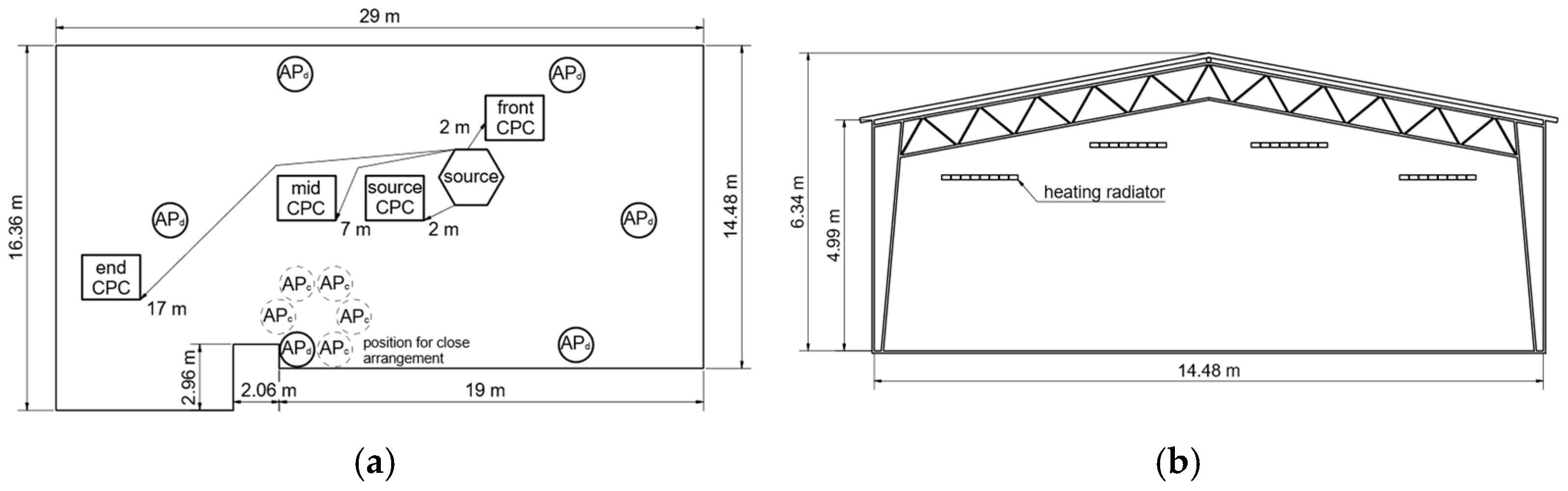
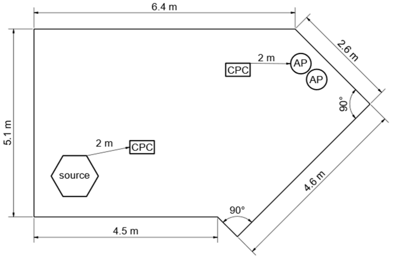
3.1. Evaluation of Mixing Quality in the Examined Spaces

Before comparing the measured concentration profiles to analytic considerations, the mixing and homogeneity of spatial particle distribution within the examined locations must be addressed. In Figure 3, the experimental results obtained in the community hall without the application of air purifiers are illustrated, and various observations can be made.

First, it takes a few minutes until an increase in particle concentration is detected by the ‘Front’ (distance of 2 m to particle source), “Mid” (distance of 7 m), and “End” (distance of 17 m) CPCs. In the first minutes of the experiment, the measured particle concentrations from the three CPCs differ slightly because there is no instant mixing. However, after 30 min at the latest, the particle concentration of the ‘Mid’ and ‘End’ CPC matches the concentration of the ‘Front CPC’ with minor, mainly statistical differences. Surprisingly, the End CPC detects particles already shortly after starting the experiment and it also detects a rise in concentration before the Front CPC, although the distance to the particle source is 17 m compared to 2 m for the Front CPC. This enormously fast response of the End CPC, combined with a non-significant difference in the measured concentration profiles at other measurement positions, must be attributed to the excellent mixing in the community hall. At the ceiling of the hall, heating radiators are installed (cf. hall cross-section in Figure 1). Since the experiments were conducted in December at an outdoor temperature of a few degrees Celsius, these radiators were running. In addition, the roof is not isolated very well, which has apparently resulted in a significant temperature gradient. It is evident that these particular conditions provided extensive convective flow circulation, and thus good mixing could unexpectedly be achieved within relatively short times, even at large distances. Furthermore, this might explain why the End CPC detected additional particles before the Front CPC, which might be caused by the vertically directed, circular flow. Overall, this illustrates that the mixing within the community hall can be considered ideal in good approximation when looking at long-term trends.

Second, the particle counter ‘Source CPC’ (cf. Figure 1a), which is also in a proximity of 2 m to the particle source, shows a significant difference in measured particle concentrations. As already mentioned in the experimental section, a compressor was used to generate the pressure required for the atomizer. When the compressor was running, additional particles were generated. Whilst the salt aerosol was emitted in the vertical direction and therefore immediately distributed to the environment, the particles generated by the compressor were obviously entrained in a directed exhaust air flow and emitted in a specific direction toward the ‘Source CPC’. This caused strong fluctuations in the corresponding concentration profile (corresponding to an operation interval around 5–6 min for the compressor), which is still clearly visible, although data are averaged in a one-minute interval. It is possible that there is also some directed macroscopic flow from the natural convection inside the hall, which would further explain why the ‘Mid’ and ‘End’ CPC showed a rise in particle concentration before the ‘Front’ CPC, which is located in the opposite direction of the particle source. To smoothen the concentration profile of the ‘Source CPC’ for a comparison to the other concentration profiles, a nine-minute averaging time was chosen for this device. Although generating additional particles by the compressor was an unintended effect, it mimics to a certain extent the real case of respiratory aerosol particle emission, which has a specific direction as well. The ‘Source’ CPC located directly in the particle stream from the compressor at a distance of 2 m measures an average particle concentration that is approximately 1.5- to 2-times higher than the mean concentration in the room. However, the ‘Front’ CPC, also at a distance of 2 m from the particle source but in the opposite direction to the particle stream from the compressor, shows almost the mean room concentration. This implies that the direction of particle emission may be more significant than the exact distance to the particle source. Even at a distance of 2 m, which is often considered as a ‘Safe Distance’, the concentration might be 1.5- to 2-times higher, if there is directional transport of the aerosol, as is typical for exhaled particles. In proximity to the particle source, the assumption of ideally mixed and homogeneously distributed particles in the room no longer applies. Referring to virus-laden aerosols, persons close to a virus-emitting person will breathe a higher concentration of harmful viruses when they stand in the direction of the exhalation flow. However, the observed additional particle generation by the compressor with directional transport can be seen as a worst-case scenario.

In the seminar room, ideal mixing could not be proven. In Figure 4, it is clearly visible that the measured concentration curves deviate depending on the CPC placement in the room. Because of the small distances in the room and the classical heat radiators located below the windows, the spikes in the particle concentration profiles caused by the compressor are still visible to some extent even in the measured concentrations close to the two air purifiers in the opposite corners of the room (cf. Figure 2), which might be due to the directed exhaust stream of the compressor.

Since the assumption of ideally mixed air is more reasonable in the community hall, most of the following considerations are related to those experiments. With a short ventilation phase after the particle source is shut down, the particle concentration in the seminar room balances and the concentration curves assimilate. This enabled decay experiments to be conducted and examined in the seminar room for an in-depth evaluation of sedimentation and aggregation, which is discussed in Section 3.3.4.

3.2. Influence of Air Purifier Power and Arrangement on Concentration Profiles

For the experiments with applied air purifiers in the community hall, the previously shown effect of almost ideal mixing was also observed. Therefore, only one representative curve averaged from the three similar concentration profiles is shown in the following considerations. In Figure 5, the experimental results for evenly distributed air purifiers at maximum power are compared to the case of distributed air purifiers at minimum power and to the case of air purifiers at maximum power in a close arrangement in one place (cf. Figure 1a).

Comparing the influence of the distribution of air purifiers, the scenario of distributed air purifiers yields a steady-state concentration of approximately 10,500 particles per cm³, while a close arrangement of air purifiers in one corner of the hall exhibits a stationary concentration of around 12,000 particles per cm³. This is an expected effect: the short distance between the closely arranged air purifiers enables bypass flows, i.e., air purifiers draw in already cleaned air, which results in a reduced effect of the CADR and consequently a higher stationary concentration. Furthermore, a reduction in fan power from level 3 to level 1 almost doubles the stationary concentration, which then amounts to 20,500 particles per cm³.

3.3. Model-Based Evaluation of Surrogate Aerosol Experiments

3.3.1. Simple Analytic Modelling of Surrogate Aerosol Experiments

When trying to assess the effectiveness of air purifiers (APs) or other measures to reduce aerosol concentrations by surrogate aerosols, experimental results are often compared to a simple model described by two terms assuming ideal mixing: the particle generator as source term $\dot{S}$ and the CADR ${\dot{V}}_{CADR}$ as the sink term if an air purifier is used. This case can be described mathematically using the differential equation:

$$V\frac{dc}{dt}=-{\dot{V}}_{CADR}c+\dot{S}$$

(1)

where $c$ denotes the concentration; $t$ is the time; and $V$ is the room volume.

Introducing a characteristic time $\tau$:

$$\tau =\frac{V}{{\dot{V}}_{CADR}}$$

(2)

where $\tau$ can be interpreted as the air purification time, i.e., the time theoretically needed for cleaning the room air once completely, if no mixing was applied.

Using Equation (2) and the assumption of $c(t=0)=0$, Equation (1) can be solved as follows:

$$c\left(t\right)=\frac{\dot{S}}{{\dot{V}}_{CADR}}\left(1-e^{-\frac{t}{\tau }}\right)=c^{*}\left(1-e^{-\frac{t}{\tau }}\right)$$

(3)

with the steady-state concentration $c^{*}$. Counter-intuitively, the room volume has no influence on this $c^{*}$. As small as the air purifier is, it will yield the same $c^{*}$ in a small seminar room as in a large community hall as long as ideal mixing is assured and other particle losses are negligible. The volume only influences the time required to achieve the steady state. The steady-state concentration, however, is solely dependent on the source strength and particle removal rate, namely CADR. This also implies that $c^{*}$ is independent of the AER. Consequently, the common recommendation during the COVID-19 pandemic, that to achieve an efficient reduction in infection risk using air purifiers required an air exchange rate between 5 h⁻¹ and 10 h⁻¹, is not supported in terms of stationary concentrations. If the indoor air is ideally mixed, the CADR cannot be derived by the common AER recommendation and needs to be evaluated individually for every case to keep aerosol concentrations below a certain value.

As explained before, the experimental results of this work show that the prerequisite of ideally mixed air is fulfilled in a good approximation, which enables a reliable comparison with the simple model, shown in Figure 6.

Comparing the experimental data to the simple model, it can be observed that starting at a concentration of around 5000 particles per cm³, the simple model deviates progressively with increasing concentrations. Note that for the simple model with applied air purifiers, a value of 340 $\frac{m^3}{h}$ for the CADR was used, as determined and explained later in this article. In this case, the same conclusion is substantiated, that particle sinks other than the CADR become relevant above particle concentrations of 5000 particles per cm³. Natural ventilation through leakage flows, deposition of particles at surfaces, aggregation, or sedimentation of particles depict further particle sinks, and their implementation into the mathematical model will be discussed in the following Section 3.3.2.

3.3.2. Extended Analytic Modelling of Surrogate Aerosol Experiments

The aforementioned phenomena of additional particle sinks can be divided into two categories. Losses due to the deposition of particles at surfaces and sedimentation are proportional to the particle concentration. Natural ventilation depends on the difference in the environmental aerosol concentration. However, since indoor surrogate aerosol concentrations are typically one or two orders of magnitude larger than outdoor concentrations, this loss mechanism can be considered with good approximation as proportional to the concentration as well. All these phenomena are considered in a kinetic coefficient $k_s$ which will be referred to as the sedimentation coefficient throughout this work because sedimentation is believed to be the dominant mechanism in most cases. However, it should always be kept in mind that this ‘sedimentation’ coefficient also reflects the aforementioned phenomena. The second category is determined by aggregation which is proportional to the squared concentration and is considered by the kinetic coefficient $k_a$.

Considering these two coefficients, the ordinary differential equation (ODE) for the theoretical description of particle concentration with surrogate aerosols in a well-mixed situation is:

$$V·\frac{dc}{dt}=-\left({Sk}_{s}c+{Vk}_a{c}^2\right)-{\dot{V}}_{CADR}c+\dot{S}$$

(4)

with $S$ denoting the room’s horizontal deposition surfaces such as tables, installations, and the floor area. However, for diffusional deposition which is also included in $k_s$, vertical walls must also be considered. Therefore, $S$ reflects a weighted mix of surfaces, being equal to the horizontal surfaces only, when sedimentation is truly the dominant linear loss mechanism. Therefore, all loss mechanisms that are linearly (or approximately linear as in the case of leakage flows) proportional to the actual concentration are summarized in one loss factor $k_l^{*}$ which is room specific because it contains different surfaces and the room volume:

$$k_l^{*}=\frac{S{k}_s}{V}$$

(5)

The first step in solving this equation is the separation of variables:

$$\underset{c_0}{\overset{c\left(t\right)}{\int }}\frac{dc}{k_a{c}^2+\left(\frac{{\dot{V}}_{CADR}}{V}+k_l^{*}\right)c-\frac{\dot{S}}{V}}=-\underset{0}{\overset{t}{\int }}dt$$

(6)

Integrating both sides of the equation leads to:

$$\frac{2ac+b-\sqrt{D}}{2ac+b+\sqrt{D}}=E{e}^{-\sqrt{D}t}$$

(7)

In Equation (7), the parameters $a$, $b,$ and $D$ were introduced to obtain a readable representation of the solution of the ODE. The three parameters are given as:

$$a=k_a$$

(8)

$$b=\left(\frac{{\dot{V}}_{CADR}}{V}+k_l^{*}\right)$$

(9)

$$D=4k_a\frac{\dot{S}}{V}+{\left(\frac{{\dot{V}}_{CADR}}{V}+k_l^{*}\right)}^2=4a\frac{\dot{S}}{V}+b^2 \mathrm{with} D>0$$

(10)

The integration constant $E$ is determined using the initial condition $\mathrm{c}\left(\mathrm{t}=0\right)={\mathrm{c}}_0$:

$$E=\frac{2a{c}_0+b-\sqrt{D}}{2a{c}_0+b+\sqrt{D}}$$

(11)

Transposing Equation (11) finally leads to the following equation which can be used to calculate the evolution of particle concentration:

$$c\left(t\right)=\frac{\left(b+\sqrt{D}\right)E{e}^{-\sqrt{D}t}-b+\sqrt{D}}{2a\left(1-E{e}^{-\sqrt{D}t}\right)}$$

(12)

A direct fit of the parameters defined in Equations (8)–(10) to the experimental data would easily allow good agreement between the model and the experimental data. However, we conducted separate experiments with the aim of determining the involved parameters individually based on physical reasoning. The respective approaches used to determine these parameters are shown in the following sections.

3.3.3. Determination of Particle Generation Rate

The measured generated particle concentration was $2\times {10}^6$ particles per cm³ in a lab setup, as described in Section 2. The particle concentration was obtained after dilution of the aerosol by an additional air gas flow of 200 L/min. Multiplying both values, a mean particle generation rate of $7\times {10}^9$ particles per second was calculated. To estimate the additional number of particles from the compressor, particle generation was evaluated by filtering the outlet air of the compressor and without the operation of the aerosol generator. Furthermore, the compressor was operated continuously instead of periodically, as in the experiments, to obtain an upper limit estimate for the particle generation rate caused by the compressor. The concentration profile of this test (corrected by the background concentration) in comparison with the experiment in the seminar room with air purifiers switched off (S_noAP) is shown in Figure 7. As can be seen, the source strength of the compressor is orders of magnitude smaller than the salt surrogate aerosol source.

This might appear surprising, considering the spikes that were detected for all experiments in proximity to the aerosol source. However, these spikes are the result of two different reasons. First, a directed flow of exhaust gas contaminated with particles contributes to these spikes, although the average total strength of this source is quite small, as shown above. Second, a significant number of particles from the compressor are contained in the air flow used to atomize the salt solution. This type of particle source from the compressor is not detected in the experiments in Figure 7 when the compressor air flow is filtered, as is the case in the experiment with the compressor only. During standard experiments and while determining the aerosol source strength, this flow is not filtered; consequently, these additionally generated particles will result in a periodic fluctuation in the aerosol source concentrations, leading to corresponding fluctuations in room concentration in the vicinity of the aerosol source. However, this type of additional particle has already been included when determining the average source strength, as described above. Thus, the comparison reveals that the number of particles generated by the compressor that were excluded from the measured source strength is minor, at a rate of 500 particles per cm³. Therefore, these additional particles are neglected, and the source strength is set to the particle generation rate of $\dot{S}=7\times {10}^9$ particles per second.

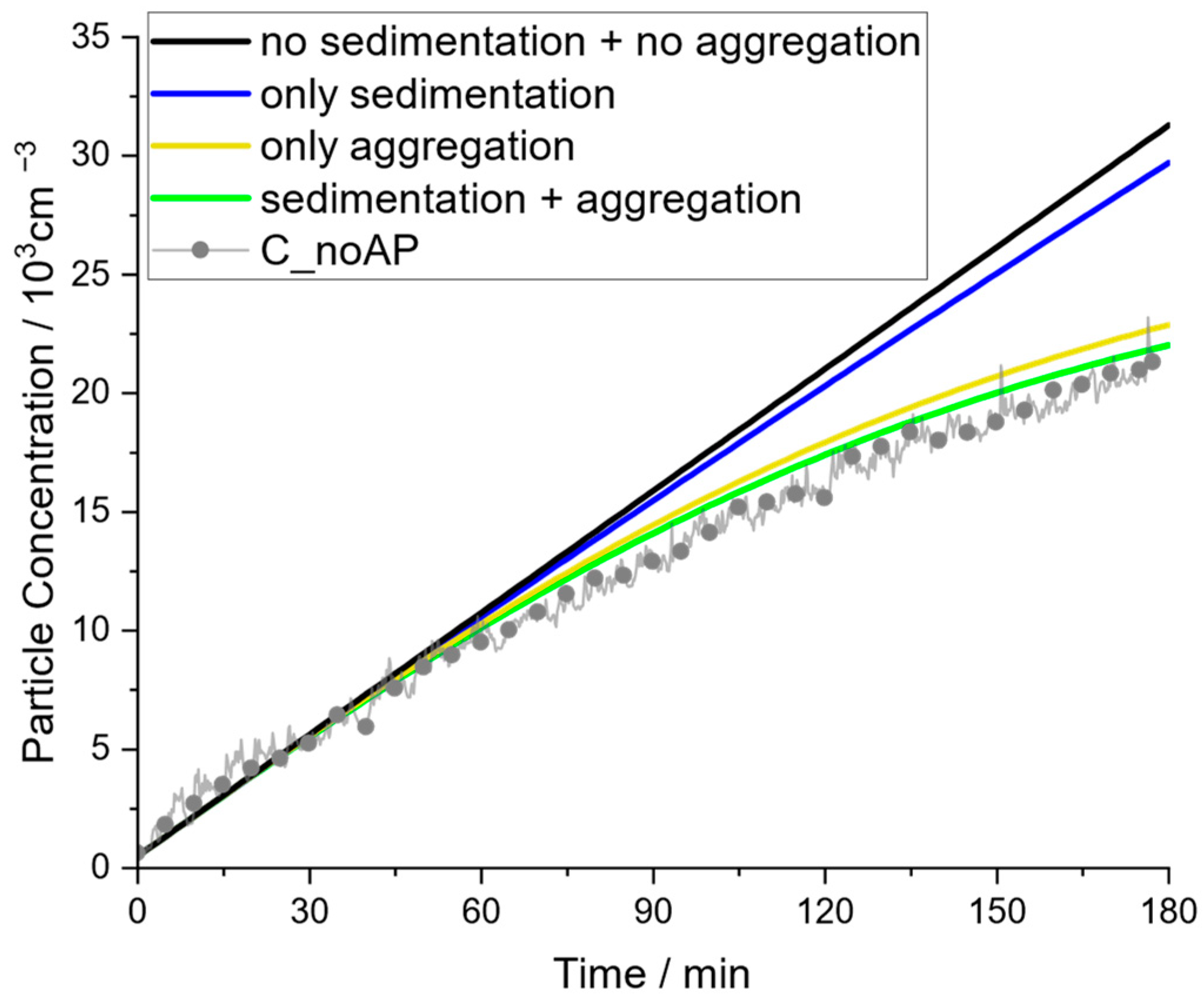
3.3.4. Consideration of Sedimentation and Aggregation

A major part of this work quantifies the relevance of sedimentation and aggregation to the obtained results. For this purpose, the kinetic coefficients $k_s$ and $k_a$ were determined experimentally by fitting the three decay experiments S_fit in the seminar room. For this fit, the ODE in Equation (4) can be simplified by setting the source strength $\dot{S}$ and the CADR ${\dot{V}}_{CADR}$ to zero. The parameters defined in Equations (8)–(10) are then:

$$a=k_a$$

(13)

$$b=k_l^{*}$$

(14)

$$D={k_l^{*}}^2$$

(15)

Integrating these parameters into Equation (12), the concentration function is simplified to:

$$\frac{c\left(t\right)}{c_0}=\frac{{\mathsf{\Pi }}_{s,0}}{\left(1+{\mathsf{\Pi }}_{s,0}\right)e^{k_l^{*}t}-1}$$

(16)

with the dimensionless ratio ${\mathsf{\Pi }}_{s,0}$ which is given by:

$${\mathsf{\Pi }}_{s,0}=\frac{k_l^{*}}{k_a{c}_0}$$

(17)

The analyzed decay data are presented in Figure 8. It shows that the data of all three experiments—each one of a ‘freshly’ produced aerosol with initial concentrations of 10,000 cm⁻³, 20,000 cm⁻³, and 30,000 cm⁻³, respectively—combine into one graph very well. This means that particle size changes due to aggregation do not significantly modify the aggregation kinetics and constant $k_a$ can be assumed under these conditions. Note that the gaps between the data points are caused by the periodically conducted SMPS measurements.

The fit of the experimental data to Equation (16) results in the values $k_l^{*}=1.14\times {10}^{-4}\frac{1}{s}$ and $k_a=3.46\times {10}^{-9}\frac{{cm}^3}{s}$ for the seminar room. In the community hall, similar experiments were conducted but only for a limited time of 30 min. The corresponding fit of Equation (16) results in $k_a=3.9\times {10}^{-9}\frac{{cm}^3}{s}$ which is in reasonable agreement with the estimation for the seminar room. Comparing both cases, the seminar room experiments cover a much broader range of concentrations for fitting the decline in concentration. Therefore, the determined value for $k_a$ in the seminar room is believed to be more accurate. Consequently, this value for $k_a$ was fixed for both cases, resulting in a value of $k_l^{*}=1.0\times {10}^{-5}\frac{1}{s}$ for the community hall. As can be seen from Figure 8, the resulting fit describes the course of the measured concentrations very well. The data scatter for the community hall appears significantly larger than in the seminar room because the scale is much larger in this case. For comparison, a linear fit of the concentrations is shown in Figure 8 for the respective cases. However, a linear fit would be obtained only if the decay is linearly proportional to the concentration, as for sedimentation, wall deposition, natural convection, etc. The obvious curvature in the measured concentration profile proves the existence of nonlinear particle sinks. A second-order loss term must be considered to represent this curvature, which leads to the conclusion that aggregation, which is proportional to the concentration squared, is a loss mechanism that cannot be neglected at such high particle concentrations.

The linear loss term $k_l^{*}$ appears to be about a factor of 10 smaller in the community hall than in the seminar room. In the case of pure sedimentation, i.e., $k_l^{*}=k_s\frac{S}{V}$, S depicts the floor area and the ratio $\frac{S}{V}$ can be simplified to $\frac{1}{H}$ with $H$ denoting the room height. Assuming pure sedimentation, the ratio of $k_l^{*}$ for both rooms should be equal to the ratio of room heights, i.e., $k_l^{*}$ in the seminar room should be larger by a factor of 2 due to the corresponding simplified geometrical considerations. However, because no ideal, empty rooms were investigated, considering only the ratio of room heights is obviously not sufficient, although this cannot explain the large deviation in the expected ratio of $k_l^{*}$ for both locations. It can be concluded that additional mechanisms are more relevant in the seminar room. When other mechanisms included in the first order loss coefficient $k_l^{*}$ are relevant, the volume $V$ cannot be considered the product of room height $H$ and surface $S$ anymore. For instance, wall deposition and installations increase $S$, while the latter also decreases $V$. Therefore, further simplifying Equation (4) or $k_l^{*}$ by including room height is not reasonable. It is likely that natural ventilation by leakage flows is the most relevant mechanism in the seminar room because old, wooden windows are installed there. In general, this underlines that the room-independent kinetic constant $k_s$ is hard to determine from isolated measurements but moreover $k_l^{*}$ has to be determined separately for any room setup by fitting concentration decay without any air purification.

The relevance of the parameters $k_l^{*}$ and $k_a$ is illustrated in Figure 9. For the experiment in the community hall with air purifiers switched off (C_noAP), the relevance of considering sedimentation and aggregation is demonstrated. The simple model would suggest a linear increase in concentration, which results in progressive deviations from the experimental data at concentrations above approximately 5000 particles per cm³. Considering sedimentation but no aggregation results in a small curvature of the concentration profile, while considering only aggregation but no sedimentation can better represent the curvature of experimental data but still overpredicts the concentration. Consequently, both mechanisms, sedimentation (or better: linear mechanisms) and aggregation, need to be considered to obtain a suitable representation of the concentration profile and neither can be neglected. This supports the hypothesis that the extended model presented in Equation (11) is an adequate mathematical approach to evaluate surrogate aerosols and should be used at least beyond 5000 particles per cm³.

To check for plausibility, the experimentally determined $k_a$ is compared with theoretical considerations. For this purpose, the approach of Lee and Chen [56] is used to calculate a theoretical aggregation coefficient. For a particle size of 100 nm (mean value of the distribution in this work), the gas-slip regime must be considered. Following their calculations, the theoretical aggregation coefficient is $k_{a,theory}\approx 1\times {10}^{-9}\frac{{cm}^3}{s}$ for a geometric standard deviation of 2, as measured in the present case (see Supplementary Materials). Comparing this simply estimated theoretical coefficient with the experimentally determined $k_a=3.46\times {10}^{-9}\frac{{cm}^3}{s}$, the presented experimental procedure can be considered an adequate approach, and the fitted $k_a$ represents a valid value for the aggregation coefficient of the surrogate aerosol.

3.3.5. Examination of the Clean Air Delivery Rate (CADR) of Applied Air Purifiers

The aim of determining all relevant model parameters based on physical reasoning also includes the CADR as it determines the steady-state concentration for the most part, as discussed earlier. Therefore, the CADRs of the air purifiers were determined experimentally instead of relying on the manufacturer’s specification that the air purifiers exhibit a CADR of $380\frac{m^3}{h}$. A fit of Equation (12) to the respective experimental data allows the determination of the corresponding CADRs, as shown in

Table 2. Experimentally determined CADRs per air purifier by evaluation according to Equation (12).

	C_maxAP_d	C_minAP_d	C_maxAP_c	S_maxAP
Start concentration/$\frac{1}{{cm}^3}$	10.000	20.000	10.000	30.000
End concentration/$\frac{1}{{cm}^3}$	7.000	18.000	7.000	4.000
Model fit CADR/$\frac{m^3}{h}$	340	65	330	290

. The CADRs are significantly below the manufacturer’s specification of 380 $\frac{m^3}{h}$. The measured CADRs with air purifiers arranged close to each other (S_maxAP with two and C_maxAP_c with six APs in close proximity each) reflect the effect of bypass flows (cf. Section 3.2). However, it appears that this effect is more important in the much smaller seminar room. In particular, the ceiling height might be important here because the air purifiers blow the cleaned air vertically upwards.

To demonstrate the accuracy of the model fit, the measured concentration profiles are depicted in Figure 10 together with the results from the extended model using the respective CADRs. Comparing the different scenarios, the extended model can describe the concentration profiles of all scenarios fairly, particularly in the case of the experiments in the community hall. For the seminar room, the model slightly underestimates the concentration; however, it needs to be considered that ideal mixing was not achieved in this case, as discussed before.

3.3.6. Comparison with the Standard Procedure of CADR Determination

As briefly outlined in the introduction, the determination of the CADR of air purifiers is also regulated by various norms (e.g., ANSI/AHAM AC-1-2020 from the US or GB/T 18801-2015 from China). The common practice of determining the CADR according to those norms deviates from the approach presented in this work, and the following section will discuss the differences in the results of the obtained CADRs.

The standard procedure always assumes an exponential decay of concentrations with time, i.e., a linear decay of the logarithmic concentration ratios. The determination of the corresponding CADR is then obtained in two steps. First, to account for any additional particle losses except removal by the air purifier, a linear decay of the concentration in the case of air purifiers switched off is assumed, which is typically referred to as natural decay. Consequently, a characteristic time, namely the natural decay time ${\tau }_n$, is determined by fitting the concentration decay (typically for 20 min) with the air purifiers switched off:

$$c_n\left(t\right)=c_0{e}^{-\frac{t}{{\tau }_n}} \mathrm{or} ln\frac{c}{c_0}=-\frac{t}{{\tau }_n}$$

(18)

This approach has also been depicted in Figure 8 and is referred to as ‘linear fit’.

Second, a fit of the experimental data with the air purifier turned on is performed in the same setup for the same time interval to obtain a characteristic decay time constant ${\tau }_{AP}$:

$$c_{AP}\left(t\right)=c_0{e}^{-\frac{t}{{\tau }_{AP}}} \mathrm{or} ln\frac{c}{c_0}=-\frac{t}{{\tau }_{AP}}$$

(19)

The overall decay in the case of air purifiers in operation is then assumed to be a superposition of the natural decay and the so-called effective decay, caused by the air purifiers only:

$$c_{AP}\left(t\right)=c_0{e}^{-\frac{t}{{\tau }_{AP}}}=c_0{e}^{-\left(\frac{1}{{\tau }_{eff}}+\frac{1}{{\tau }_n}\right)t}$$

(20)

Because any characteristic decay time can be associated with a corresponding CADR-value, one can obtain the effective CADR straightforwardly:

$${CADR}_{eff}=CAD{R}_{AP}-CAD{R}_n \mathrm{with} \mathrm{each} CAD{R}_i=\frac{V}{{\tau }_i}$$

(21)

However, as shown in Figure 8, the natural decay is not linear. Moreover, the effect of aggregation, which is proportional to the concentration squared, causes a curvature in the logarithmic concentration decay. Therefore, an ‘actual’ natural decay rate is calculated by determining the derivative from Equation (16), as fitted to the experimental data and parameters according to Section 3.3.4. As shown in Figure 11, the calculated actual decay rate strongly depends on the actual concentration. While aggregation (given by the term $k_a{c}^2$) is assumed to be independent of the respective room, the other linear natural decay mechanisms (hence given by the term $k_l^{*}c$) may strongly depend on the respective setting. Since the value of $k_l^{*}$ in the seminar room is an order of magnitude larger than that in the community hall, the natural decay rate in the seminar room is also significantly larger. However, the natural decay rate $1/{\tau }_n$ in the seminar room increases by about a factor of 2 for the concentration increasing to $3\times {10}^5\mathrm{c}{\mathrm{m}}^{-3}$, while it increases by more than a factor of 10 in the case of the community hall. This reflects the much larger impact in the case of the community hall, since the ratio of aggregation kinetics to other decay mechanisms (linearly depending on concentration) is much larger. Furthermore, Figure 11 shows the corresponding CADR_n calculated according to Equation (21). It clearly shows the much larger effect of natural decay in the case of the huge volume there. This indicates that a large volume is unfavorable for determining the CADR of air purifiers with high accuracy.

Applying the ‘standard method’ to determine the CADR requires a linear fit of the logarithmic concentration decay, averaging the decreasing slope due to the declining aggregation with reducing concentration. However, since typically both measurements, i.e., decay with air purifiers on and off, respectively, are performed for the same time interval, the final concentration with air purifiers switched off is significantly higher compared to the case when air purifiers are switched on. Therefore, because of the higher average concentration during the natural decay measurement, aggregation is stronger in this case. Therefore, a systematic overestimation of the natural CADR_n and consequently a systematic underprediction of the effective CADR_eff can be expected. Furthermore, it can be expected that this effect is even more pronounced for longer time intervals of the decay measurement.

This systematic error can be evaluated for the measurements described above. Figure 12 shows the respective concentration profiles. To eliminate errors due to measurement fluctuations, fitted data instead of actual experimental data are used here. It should be noted that the different experiments started at quite different initial concentrations, and the different air exchange rates in both rooms resulted in a significantly differing decline in concentration. These data and the respective data from natural decay (cf. Figure 11) can be used to determine the CADR_eff by applying Equations (18), (19), and (21) for varying time intervals and alternatively using the CADR from Table 2, determined by fitting Equation (12), as reference. The relative deviation $D$ is then calculated as:

$$D=\frac{CAD{R}_{fit}-CAD{R}_{eff}\left(t\right)}{CAD{R}_{fit}}$$

(22)

This deviation is also shown in Figure 12. All deviations are positive, which confirms the assumption that the standard method systematically underestimates the CADR value. Comparing the deviation for the two experiments in the community hall shows that the higher concentration in the experiment with a low fan level (C_minAP_d) results in significantly higher deviations. This can be explained by the larger impact of aggregation for higher particle concentrations and the fact that the deviation $D$ is a relative deviation, i.e., for a higher CADR, even the same absolute error would result in a smaller relative error. The experiments in the seminar room are characterized by a very high initial concentration followed by a strong decline due to the high air exchange ratio. For short time intervals, a very high gradient in particle concentration exists, which in this case leads to deviations comparable to those in the community hall with a low fan level (C_minAP_d). However, for larger evaluation times, it exhibits a maximum followed by a negligible decline.

To better understand the influence of experimental conditions and evaluation on the obtained CADR values, a systematic parameter study was performed, as shown in Figure 13. Here, the deviation $D$ is depicted as a contour plot depending on the air exchange rate $\dot{V}/V$ and the evaluation time used to determine the CADR (which is 20 min for the norm case as reference).

Again, all deviations are positive, confirming that the discussed effect leads to a systematic underestimation of the CADR using the ‘standard method’. The diagrams a–c are determined for parameters reflecting the situation in the seminar room, i.e., a case with rather high $k_l^{*}$ with the varying initial concentration $c_0$. It can be clearly seen that for high air exchange rates, the error is rather low. Even for very high initial concentrations of $5\times {10}^4$ cm⁻³, the deviation never exceeds 5%. However, for small exchange rates, the relative deviation increases significantly. At first glance, this might appear counter intuitive: the steeper the gradient in concentration, i.e., high exchange rates, the stronger the effect of different aggregation kinetics for air purifiers switched on and off, respectively. Consequently, the absolute deviation is larger in the case of high air exchange rates. However, the deviation $D$ is related to the actual CADR, which obviously overcompensates for the increasing deviation. Consequently, for small air exchange rates, particularly below around 2 h⁻¹, the deviation is strongly increasing with increasing evaluation time intervals and might reach values even higher than 10%. For high air exchange rates, one can observe a maximum deviation for medium evaluation time intervals, as shown in Figure 12. This can be explained by the fact that, in these cases, concentrations become so low after some time that aggregation is not relevant at all. Therefore, concentrations during the natural decay experiments with longer evaluation times will reflect this situation better. Hence, the deviation decreases for longer time intervals.

Comparing Figure 13a,d reveals that the difference in $k_l^{*}$ does not change much in the deviation, although aggregation is much more relevant than settling in the second case. However, if the decay due to air purifiers is stronger than the natural decay, the ratio of aggregation, which is the reason for any deviation discussed here, to air removal is more relevant.

Finally, Figure 13e,f show the deviation with respect to the initial concentration and air exchange rate for 20 min and 60 min evaluation time intervals, respectively. The deviation for 20 min is below 5% in most relevant cases because the concentration should be kept below $5\times {10}^5$ cm⁻³ because this is the limit for the CPC to operate in counting mode. Although 20 min is the standard time interval proposed in the norms, for the evaluation of aerosol dynamics in a room longer times might be of interest. Therefore, diagram f shows the deviation for the 60 min evaluation time. In this case, the deviation is significantly higher and might even exceed 10%.

All deviations discussed above are due to different concentrations in the experiments with and without air purifiers in operation. Therefore, a longer natural decay experiment with initial and final concentrations identical to the respective decay experiments with an air purifier provides a remedy. Simulations for all situations shown above revealed deviations less than 1% in any case, if the natural decay is not determined for the same time interval but for the same concentration ratio as the decay experiment with air purifiers.

4. Discussion

When measurements of aerosol dynamics in confined spaces are performed using surrogate aerosol particles, it is important to provide rather high concentrations to minimize errors by background aerosol sources. Measurements in different settings (large community hall and small seminar room) show that aggregation becomes relevant at least for concentrations exceeding 5000 cm⁻³. An extended model for the well-mixed case proves to be surprisingly well suited to describe the measured concentration course, at least for the community hall, suggesting a well-mixed situation. All relevant model parameters (source strength, CADR, kinetic coefficients for aggregation, and linear decay mechanisms) were determined experimentally independently and implemented into the extended model. This adjusted theoretical model describes the concentrations of surrogate aerosols fairly.

For the seminar room, however, some small discrepancies were detected, which can be attributed to a lack of ideal mixing in this case. Therefore, for well-mixed enclosed spaces, the adequacy of the extended model is validated. It enables better representation of the curvature of concentration profiles at high particle concentrations (cf. also Figure 6 for comparison with the simple model), which are typical for surrogate aerosol experiments. This leads to a more accurate prediction of the steady-state concentration. Therefore, applying an extended model for surrogate aerosol experiments instead of the simple model is highly recommended at high particle concentrations.

It should be considered that the linear decay coefficient $k_l^{*}$ includes all effects that are proportional to the actual particle concentration. It is expected to depend on the surface-to-volume ratio, the geometry of the room (e.g., horizontal planes like tables which remove additional particles due to settling, all other surfaces), leakage flows, and particle size distribution. In contrast, the aggregation coefficient $k_a$ should only depend on the particle size distribution, i.e., larger values for broader size distributions and, in most cases, slightly higher values for smaller particles. Therefore, these constants must be determined depending on the particle source and the conditions in the respective room.

In addition to the consideration of aerosol dynamics in indoor spaces, these findings have implications for the determination of the clean air delivery rate (CADR) of air purifiers. They are typically examined in test chambers with surrogate aerosols as well. The standard procedure using linear fits of the logarithmic concentration decay with and without air purifiers in operation neglects the influence of the quadratic dependence of aggregation on concentration. In the case of an evaluation time interval of 20 min and a maximum concentration of 20,000 cm⁻³, as proposed in, e.g., the Chinese norm, the associated error might be considered minor. Nevertheless, for longer time intervals and higher concentrations, this is not the case anymore. In these cases, it is advisable to use the presented extended model or to determine the natural decay for the identical concentration range as the overall decay rather than the identical evaluation time to avoid this error.

5. Conclusions

In the scope of this work, experiments were conducted to observe particle concentrations by surrogate aerosols generated via an atomizer mimicking a steady particle emitter. It was shown that aerosols can spread rapidly in enclosed spaces when the room volume is well mixed. In only a few minutes, even a large community hall can depict an almost uniform aerosol concentration. This implies that the inhaled dose of aerosol particles is almost the same for all persons staying in the room, independent of the distance to the emitter. People in very close distances in the direction of exhaled air will face a slightly higher concentration, about 1.5 to 2 times higher than the average, at a distance of 2 m, which is reasonable enough to consider this an adequate ‘safe distance’.

The approach of tracking particle concentrations by means of surrogate aerosols involves high particle concentrations, and this study showed that the simple model with only the atomizer as particle source and air purifiers as particle sink does not represent concentration profiles at elevated concentrations above 5000 particles per cm³ in good approximation. For a more precise model description of the concentration profiles, additional effects such as sedimentation and aggregation need to be considered. For both effects, kinetic coefficients were determined from independent measurements and inserted into the model to obtain a more representative theoretical description of the experimental data. In addition, the atomizer’s particle generation rate and the CADR of the applied air purifiers were determined experimentally by fitting the respective parameter in the derived model equation.

In the case of CADR determination, it was shown that the CADR was below the manufacturer’s specification, although brand-new devices were used. Furthermore, some influence of bypass flows could be observed if the air purifiers are operated in close proximity.

Overall, all relevant model parameters (source strength, kinetic coefficients for sedimentation and aggregation, and CADRs) were determined independently, and their insertion into an extended model led to an accurate representation of the long-term concentration profiles and steady-state concentrations.

The effect of aggregation causes a deviation of the concentration from an exponential decay because it is proportional to the actual concentration squared. Therefore, it is shown that standard evaluation procedures for CADR do not adequately cover this effect. The resulting deviation causes a systematic underestimation of the CADR, and this effect increases with lower air exchange rates, higher initial concentrations, and longer evaluation time intervals. While for conditions as proposed in the norms, the deviation is typically below 5%, it might become significantly larger and highly relevant if conditions are present, which are more likely to apply to surrogate aerosol measurements in indoor spaces. However, these errors can be avoided by using the proposed extended model or by determining natural decay rates for identical concentration ratios compared with the decay with air purifiers instead of applying identical evaluation time intervals.

To transfer experiments with surrogate aerosol particles to the spreading of virus-laden respiratory aerosols, it is important to note that they do not behave identically. In particular, aggregation is relevant for surrogate aerosols (at least if concentrations above 5000 particles per cm³ are applied) but not for respiratory aerosols, since for the latter, typical particle concentrations are much lower. However, linear decay mechanisms are relevant for both types of aerosols. To have comparable values for $k_l^{*}$ in both cases, it is essential that the size distributions of surrogate and respiratory particle sizes are as similar as possible. To predict infection risks, the concentrations of contagious viruses must be calculated based on the approach presented in this paper. Experiments with surrogate aerosols allow the determination of $k_l^{*}$. The source strength must be assumed to depend on the number of infected people and their activities. Furthermore, an additional decay mechanism must be added to account for natural airborne virus deactivation [57]. Because this deactivation rate is also proportional to the number of active pathogens, the deactivation rate constant can be added to $k_l^{*}$. Overall, the presented extended model can be used for deductions of virus-laden respiratory aerosols if the corresponding adaptations of the parameters obtained from the surrogate aerosol experiments are considered.

References

1. Zhu, N.; Zhang, D.; Wang, W.; Li, X.; Yang, B.; Song, J.; Zhao, X.; Huang, B.; Shi, W.; Lu, R.; et al. A Novel Coronavirus from Patients with Pneumonia in China, 2019. N. Engl. J. Med. 2020, 382, 727–733. [Google Scholar] [CrossRef] [PubMed]
2. Laue, M.; Kauter, A.; Hoffmann, T.; Möller, L.; Michel, J.; Nitsche, A. Morphometry of SARS-CoV and SARS-CoV-2 particles in ultrathin plastic sections of infected Vero cell cultures. Sci. Rep. 2021, 11, 3515. [Google Scholar] [CrossRef] [PubMed]
3. Scheuch, G. Breathing Is Enough: For the Spread of Influenza Virus and SARS-CoV-2 by Breathing Only. J. Aerosol Med. Pulm. Drug Deliv. 2020, 33, 230–234. [Google Scholar] [CrossRef] [PubMed]
4. Asadi, S.; Wexler, A.S.; Cappa, C.D.; Barreda, S.; Bouvier, N.M.; Ristenpart, W.D. Aerosol emission and superemission during human speech increase with voice loudness. Sci. Rep. 2019, 9, 2348. [Google Scholar] [CrossRef] [PubMed]
5. Han, Z.Y.; Weng, W.G.; Huang, Q.Y. Characterizations of particle size distribution of the droplets exhaled by sneeze. J. R. Soc. Interface 2013, 10, 20130560. [Google Scholar] [CrossRef]
6. Hartmann, A.; Lange, J.; Rotheudt, H.; Kriegel, M. Emissionsrate und Partikelgröße von Bioaerosolen beim Atmen, Sprechen und Husten; Technische Universität Berlin: Berlin, Germany, 2020. [Google Scholar] [CrossRef]
7. Haslbeck, K.; Schwarz, K.; Hohlfeld, J.M.; Seume, J.R.; Koch, W. Submicron droplet formation in the human lung. J. Aerosol Sci. 2010, 41, 429–438. [Google Scholar] [CrossRef]
8. Papineni, R.S.; Rosenthal, F.S. The size distribution of droplets in the exhaled breath of healthy human subjects. J. Aerosol Med. Off. J. Int. Soc. Aerosols Med. 1997, 10, 105–116. [Google Scholar] [CrossRef]
9. Schwarz, K.; Biller, H.; Windt, H.; Koch, W.; Hohlfeld, J.M. Characterization of exhaled particles from the healthy human lung—A systematic analysis in relation to pulmonary function variables. J. Aerosol Med. Pulm. Drug Deliv. 2010, 23, 371–379. [Google Scholar] [CrossRef] [PubMed]
10. Xie, X.; Li, Y.; Sun, H.; Liu, L. Exhaled droplets due to talking and coughing. J. R. Soc. Interface 2009, 6 (Suppl. S6), S703–S714. [Google Scholar] [CrossRef]
11. Xie, X.; Li, Y.; Chwang, A.T.Y.; Ho, P.L.; Seto, W.H. How far droplets can move in indoor environments--revisiting the Wells evaporation-falling curve. Indoor Air 2007, 17, 211–225. [Google Scholar] [CrossRef] [PubMed]
12. GAeF. Position Paper on Aerosols and SARS-CoV-2. Available online: https://www.info.gaef.de/position-paper (accessed on 23 November 2023).
13. Smither, S.J.; Eastaugh, L.S.; Findlay, J.S.; Lever, M.S. Experimental aerosol survival of SARS-CoV-2 in artificial saliva and tissue culture media at medium and high humidity. Emerg. Microbes Infect. 2020, 9, 1415–1417. [Google Scholar] [CrossRef] [PubMed]
14. van Doremalen, N.; Bushmaker, T.; Morris, D.H.; Holbrook, M.G.; Gamble, A.; Williamson, B.N.; Tamin, A.; Harcourt, J.L.; Thornburg, N.J.; Gerber, S.I.; et al. Aerosol and Surface Stability of SARS-CoV-2 as Compared with SARS-CoV-1. N. Engl. J. Med. 2020, 382, 1564–1567. [Google Scholar] [CrossRef] [PubMed]
15. Zhang, R.; Li, Y.; Zhang, A.L.; Wang, Y.; Molina, M.J. Identifying airborne transmission as the dominant route for the spread of COVID-19. Proc. Natl. Acad. Sci. USA 2020, 117, 14857–14863. [Google Scholar] [CrossRef] [PubMed]
16. Wang, C.C.; Prather, K.A.; Sznitman, J.; Jimenez, J.L.; Lakdawala, S.S.; Tufekci, Z.; Marr, L.C. Airborne transmission of respiratory viruses. Science 2021, 373, eabd9149. [Google Scholar] [CrossRef] [PubMed]
17. Morawska, L.; Cao, J. Airborne transmission of SARS-CoV-2: The world should face the reality. Environ. Int. 2020, 139, 105730. [Google Scholar] [CrossRef]
18. Coronavirus Disease (COVID-19): How Is It Transmitted? Available online: https://www.who.int/news-room/questions-and-answers/item/coronavirus-disease-covid-19-how-is-it-transmitted (accessed on 23 November 2023).
19. Adzic, F.; Roberts, B.M.; Hathway, E.A.; Kaur Matharu, R.; Ciric, L.; Wild, O.; Cook, M.; Malki-Epshtein, L. A post-occupancy study of ventilation effectiveness from high-resolution CO2 monitoring at live theatre events to mitigate airborne transmission of SARS-CoV-2. Build. Environ. 2022, 223, 109392. [Google Scholar] [CrossRef]
20. Zhao, Y.; Gu, C.; Song, X. Evaluation of indoor environmental quality, personal cumulative exposure dose, and aerosol transmission risk levels inside urban buses in Dalian, China. Environ. Sci. Pollut. Res. Int. 2023, 30, 55278–55297. [Google Scholar] [CrossRef]
21. Iwamura, N.; Tsutsumi, K. SARS-CoV-2 airborne infection probability estimated by using indoor carbon dioxide. Environ. Sci. Pollut. Res. Int. 2023, 30, 79227–79240. [Google Scholar] [CrossRef] [PubMed]
22. Vassella, C.C.; Koch, J.; Henzi, A.; Jordan, A.; Waeber, R.; Iannaccone, R.; Charrière, R. From spontaneous to strategic natural window ventilation: Improving indoor air quality in Swiss schools. Int. J. Hyg. Environ. Health 2021, 234, 113746. [Google Scholar] [CrossRef] [PubMed]
23. Kumar, P.; Rawat, N.; Tiwari, A. Micro-characteristics of a naturally ventilated classroom air quality under varying air purifier placements. Environ. Res. 2023, 217, 114849. [Google Scholar] [CrossRef]
24. Alegría-Sala, A.; Clèries Tardío, E.; Casals, L.C.; Macarulla, M.; Salom, J. CO2 Concentrations and Thermal Comfort Analysis at Onsite and Online Educational Environments. Int. J. Environ. Res. Public Health 2022, 19, 16039. [Google Scholar] [CrossRef]
25. Di Gilio, A.; Palmisani, J.; Pulimeno, M.; Cerino, F.; Cacace, M.; Miani, A.; de Gennaro, G. CO2 concentration monitoring inside educational buildings as a strategic tool to reduce the risk of Sars-CoV-2 airborne transmission. Environ. Res. 2021, 202, 111560. [Google Scholar] [CrossRef]
26. Rudnick, S.N.; Milton, D.K. Risk of indoor airborne infection transmission estimated from carbon dioxide concentration. Indoor Air 2003, 13, 237–245. [Google Scholar] [CrossRef]
27. Peng, Z.; Jimenez, J.L. Exhaled CO2 as a COVID-19 Infection Risk Proxy for Different Indoor Environments and Activities. Environ. Sci. Technol. Lett. 2021, 8, 392–397. [Google Scholar] [CrossRef]
28. Bazant, M.Z.; Kodio, O.; Cohen, A.E.; Khan, K.; Gu, Z.; Bush, J.W. Monitoring carbon dioxide to quantify the risk of indoor airborne transmission of COVID-19. Flow 2021, 1, E10. [Google Scholar] [CrossRef]
29. Schade, W.; Reimer, V.; Seipenbusch, M.; Willer, U. Experimental Investigation of Aerosol and CO2 Dispersion for Evaluation of COVID-19 Infection Risk in a Concert Hall. Int. J. Environ. Res. Public Health 2021, 18, 3037. [Google Scholar] [CrossRef] [PubMed]
30. Duill, F.F.; Schulz, F.; Jain, A.; van Wachem, B.; Beyrau, F. Comparison of Portable and Large Mobile Air Cleaners for Use in Classrooms and the Effect of Increasing Filter Loading on Particle Number Concentration Reduction Efficiency. Atmosphere 2023, 14, 1437. [Google Scholar] [CrossRef]
31. Burgmann, S.; Janoske, U. Transmission and reduction of aerosols in classrooms using air purifier systems. Phys. Fluids 2021, 33, 33321. [Google Scholar] [CrossRef] [PubMed]
32. Duill, F.F.; Schulz, F.; Jain, A.; Krieger, L.; van Wachem, B.; Beyrau, F. The Impact of Large Mobile Air Purifiers on Aerosol Concentration in Classrooms and the Reduction of Airborne Transmission of SARS-CoV-2. Int. J. Environ. Res. Public Health 2021, 18, 11523. [Google Scholar] [CrossRef] [PubMed]
33. Szabadi, J.; Meyer, J.; Lehmann, M.; Dittler, A. Simultaneous temporal, spatial and size-resolved measurements of aerosol particles in closed indoor environments applying mobile filters in various use-cases. J. Aerosol Sci. 2022, 160, 105906. [Google Scholar] [CrossRef]
34. Curtius, J.; Granzin, M.; Schrod, J. Testing mobile air purifiers in a school classroom: Reducing the airborne transmission risk for SARS-CoV-2. Aerosol Sci. Technol. 2021, 55, 586–599. [Google Scholar] [CrossRef]
35. Kähler, C.J.; Hain, R.; Fuchs, T. Assessment of Mobile Air Cleaners to Reduce the Concentration of Infectious Aerosol Particles Indoors. Atmosphere 2023, 14, 698. [Google Scholar] [CrossRef]
36. Kähler, C.J.; Fuchs, T.; Mutsch, B.; Hain, R. School education during the SARS-CoV-2 pandemic—Which concept is safe, feasible and environmentally sound? medRxiv 2020. [Google Scholar] [CrossRef]
37. Küpper, M.; Asbach, C.; Schneiderwind, U.; Finger, H.; Spiegelhoff, D.; Schumacher, S. Testing of an Indoor Air Cleaner for Particulate Pollutants under Realistic Conditions in an Office Room. Aerosol Air Qual. Res. 2019, 19, 1655–1665. [Google Scholar] [CrossRef]
38. Dbouk, T.; Roger, F.; Drikakis, D. Reducing indoor virus transmission using air purifiers. Phys. Fluids 2021, 33, 103301. [Google Scholar] [CrossRef] [PubMed]
39. Quintero, F.; Nagarajan, V.; Schumacher, S.; Todea, A.M.; Lindermann, J.; Asbach, C.; Luzzato, C.M.A.; Jilesen, J. Reducing Particle Exposure and SARS-CoV-2 Risk in Built Environments through Accurate Virtual Twins and Computational Fluid Dynamics. Atmosphere 2022, 13, 2032. [Google Scholar] [CrossRef]
40. Sabanskis, A.; Vidulejs, D.D.; Teličko, J.; Virbulis, J.; Jakovičs, A. Numerical Evaluation of the Efficiency of an Indoor Air Cleaner under Different Heating Conditions. Atmosphere 2023, 14, 1706. [Google Scholar] [CrossRef]
41. Srivastava, S.; Zhao, X.; Manay, A.; Chen, Q. Effective ventilation and air disinfection system for reducing coronavirus disease 2019 (COVID-19) infection risk in office buildings. Sustain. Cities Soc. 2021, 75, 103408. [Google Scholar] [CrossRef] [PubMed]
42. Tobisch, A.; Springsklee, L.; Schäfer, L.-F.; Sussmann, N.; Lehmann, M.J.; Weis, F.; Zöllner, R.; Niessner, J. Reducing indoor particle exposure using mobile air purifiers-Experimental and numerical analysis. AIP Adv. 2021, 11, 125114. [Google Scholar] [CrossRef]
43. Foster, A.; Kinzel, M. Estimating COVID-19 exposure in a classroom setting: A comparison between mathematical and numerical models. Phys. Fluids 2021, 33, 021904. [Google Scholar] [CrossRef]
44. Schumacher, S.; Schmid, H.-J.; Asbach, C. Gefahrstoffe. GrdL 2021, 81, 16–28. [Google Scholar] [CrossRef]
45. Manoukian, A.; Quivet, E.; Temime-Roussel, B.; Nicolas, M.; Maupetit, F.; Wortham, H. Emission characteristics of air pollutants from incense and candle burning in indoor atmospheres. Environ. Sci. Pollut Res 2013, 20, 4659–4670. [Google Scholar] [CrossRef]
46. Bivolarova, M.; Ondráček, J.; Melikov, A.; Ždímal, V. A comparison between tracer gas and aerosol particles distribution indoors: The impact of ventilation rate, interaction of airflows, and presence of objects. Indoor Air 2017, 27, 1201–1212. [Google Scholar] [CrossRef]
47. Chan, W.R.; Logue, J.M.; Wu, X.; Klepeis, N.E.; Fisk, W.J.; Noris, F.; Singer, B.C. Quantifying fine particle emission events from time-resolved measurements: Method description and application to 18 California low-income apartments. Indoor Air 2018, 28, 89–101. [Google Scholar] [CrossRef] [PubMed]
48. ANSI/AHAM AC-1-2020; Method for Measuring Performance of Portable Household Electric Room Air Cleaners. American National Standards Institute (ANSI): Washington, DC, USA; Association of Home Appliance Manufacturers (AHAM): Washington, DC, USA, 2020.
49. GB/T 18801-2015; Air Cleaner. Standardization Administration of the People’s Republic of China: Beijing, China, 2015.
50. Burdack-Freitag, A.; Buschhaus, M.; Grün, G.; Hofbauer, W.K.; Johann, S.; Nagele-Renzl, A.M.; Schmohl, A.; Scherer, C.R. Particulate Matter versus Airborne Viruses—Distinctive Differences between Filtering and Inactivating Air Cleaning Technologies. Atmosphere 2022, 13, 1575. [Google Scholar] [CrossRef]
51. Schmohl, A.; Buschhaus, M.; Norrefeldt, V.; Johann, S.; Burdack-Freitag, A.; Scherer, C.R.; Vega Garcia, P.A.; Schwitalla, C. Incremental Evaluation Model for the Analysis of Indoor Air Measurements. Atmosphere 2022, 13, 1655. [Google Scholar] [CrossRef]
52. Nazaroff, W.W.; Cass, G.R. Mathematical modeling of indoor aerosol dynamics. Environ. Sci. Technol. 1989, 23, 157–166. [Google Scholar] [CrossRef]
53. Nazaroff, W.W. Indoor particle dynamics. Indoor Air 2004, 14 (Suppl. S7), 175–183. [Google Scholar] [CrossRef] [PubMed]
54. Nazaroff, W.W. Indoor bioaerosol dynamics. Indoor Air 2016, 26, 61–78. [Google Scholar] [CrossRef]
55. Schumacher, S.; Banda Sanchez, A.; Caspari, A.; Staack, K.; Asbach, C. Testing Filter-Based Air Cleaners with Surrogate Particles for Viruses and Exhaled Droplets. Atmosphere 2022, 13, 1538. [Google Scholar] [CrossRef]
56. Lee, K.W.; Chen, H. Coagulation Rate of Polydisperse Particles. Aerosol Sci. Technol. 1984, 3, 327–334. [Google Scholar] [CrossRef]
57. Biryukov, J.; Boydston, J.A.; Dunning, R.A.; Yeager, J.J.; Wood, S.; Reese, A.L.; Ferris, A.; Miller, D.; Weaver, W.; Zeitouni, N.E.; et al. Increasing Temperature and Relative Humidity Accelerates Inactivation of SARS-CoV-2 on Surfaces. mSphere 2020, 5. [Google Scholar] [CrossRef] [PubMed]
Figure 1. (a) Community hall setup with positions of aerosol source, APs (in two alternative configurations), and CPCs; (b) vertical cross-section of the community hall with marked ceiling heating radiators.
Atmosphere 15 00305 g001
Figure 2. Seminar room setup with positions of the aerosol source, APs, and CPCs.
Atmosphere 15 00305 g002
Figure 3. Concentration profiles for experiment C_noAP (community hall without APs, measured at different locations according to Figure 1).
Atmosphere 15 00305 g003
Figure 4. Measured concentration profiles of experiment S_noAP (seminar room, air purifiers out of operation).
Atmosphere 15 00305 g004
Figure 5. Concentration profiles of experiments with operating air purifiers in different configurations at the community hall: APs distributed and operated at level 1 (C_minAP_d); APs arranged close together and operated at level 3 (C_maxAP_c); APs distributed and operated at level 3 (C_maxAP_d).
Atmosphere 15 00305 g005
Figure 6. Comparison of experimental data to the predicted values by the simple model for the scenarios in the community hall with air purifiers running at the highest level (C_maxAP_d) and shut down (C_noAP).
Atmosphere 15 00305 g006
Figure 7. Comparison of the increase in room concentration for experiment S_noAP and pure particle generation by the compressor during continuous operation.
Atmosphere 15 00305 g007
Figure 8. Fitted experimental data for determination of kinetic parameters for sedimentation and aggregation in the seminar room (left), and in the community hall (right); k a = 3.46 × 10 9 c m 3 s ;   k l * fitted individually.
Atmosphere 15 00305 g008
Figure 9. Influence of aggregation and sedimentation on resembling experimental data for the scenario in the community hall with APs switched off (C_noAP).
Atmosphere 15 00305 g009
Figure 10. Comparison of measured data with the extended model with independently determined model parameters.
Atmosphere 15 00305 g010
Figure 11. Natural decay in different settings (seminar room and community hall) with respect to the actual concentration: natural decay rate (left) and corresponding CADRn (right).
Atmosphere 15 00305 g011
Figure 12. Time-dependent concentration (fitted) for three different cases (green) and deviation D of obtained CADR from fit to extended model (Equation (12)) compared with the CADR determined by the ‘standard procedure’ with respect to the applied time interval (Equations (18), (19), and (21)) (blue).
Atmosphere 15 00305 g012
Figure 13. The calculated relative deviation D in % is depicted as isolines for determination of CADR by ‘standard procedure’ (Equations (18), (19), and (21)) for k a = 3.46 × 10 9 c m 3 s and given parameters of k l * ,   c 0 and concentrations assessed for an evaluation time interval t (Equation (20)) referenced to the CADR determined by fitting to the extended model (Equation (11)). High settling constant k l *   (ac,e,f) corresponds to conditions in the seminar room, low k l * (d) corresponds to community hall.
Atmosphere 15 00305 g013