Article

Using Diverse Data Sources to Impute Missing Air Quality Data Collected in a Resource-Limited Setting

by
Moses Mogakolodi Kebalepile
1,*,
Loveness Nyaradzo Dzikiti
2,3 and
Kuku Voyi
2
1
School of Clinical Medicine, University of the Witwatersrand, Johannesburg 2050, South Africa
2
School of Health Systems and Public Health, University of Pretoria, Pretoria 0007, South Africa
3
Ross University School of Veterinary Medicine, Basseterre P.O. Box 334, Saint Kitts and Nevis
*
Author to whom correspondence should be addressed.
Atmosphere 2024, 15(3), 303; https://doi.org/10.3390/atmos15030303
Submission received: 24 November 2023 / Revised: 5 February 2024 / Accepted: 27 February 2024 / Published: 28 February 2024
(This article belongs to the Special Issue Machine Learning in Air Pollution)

Abstract

:
The sustainable operation of ambient air quality monitoring stations in developing countries is not always possible. Intermittent failures and breakdowns at air quality monitoring stations often affect the continuous measurement of data as required. These failures and breakdowns result in missing data. This study aimed to impute NO2, SO2, O3, and PM 10 to produce complete data sets of daily average exposures from 2010 to 2017. Models were built for (a) an individual pollutant at a monitoring station, (b) a combined model for the same pollutant from different stations, and (c) a data set with all the pollutants from all the monitoring stations. This study sought to evaluate the efficacy of the Multiple Imputation by Chain Equations (MICE) algorithm in successfully imputing air quality data that are missing at random. The application of classification and regression trees (CART) analysis using the MICE package in the R statistical programming language was compared with the predictive mean matching (PMM) method. The CART method performed better, with the pooled R-squared statistics of the imputed data ranging from 0.3 to 0.7, compared to a range of 0.02 to 0.25 for PMM. The MICE algorithm successfully resolved the incompleteness of the data. It was concluded that the CART method produced better reliable data than the PMM method. However, in this study, the pooled R2 values were accurate for NO2, but not so much for other pollutants.

1. Introduction

The World Health Organization (WHO) documents that healthier environments, such as those with clean air, have the potential to reduce the global burden of disease by nearly a quarter [1,2]. Therefore, the organization has recommendations and action plans prescribed for the mitigation of environmental pollutants and directives for the maintenance of healthier environments [3,4,5]. Following the statutes, recommendations, and guidelines of the WHO, South Africa has adopted a strategic national action plan prepared to ensure healthier environments. Concerning air quality, the National Framework for Air Quality Management in the Republic of South Africa requires that air quality be monitored using acceptable methods and that compliance with national standards is mandatory [6]. However, the sustainable operation of ambient air quality monitoring stations in South Africa has not always been possible. Intermittent failures and breakdowns at the monitoring stations have often affected the continuous measurement of data as required. These failures in the running of monitoring stations result in missing data, and this incompleteness of data can present limitations and prevent public health research that studies environmental health, environmental epidemiology, and environmental toxicology. This study seeks to evaluate the efficacy of a data imputation approach using two methods (CART and PMM) applied using the MICE package.
As an outcome of the requirements of the South African National Environmental Management: Air Quality Act, of 2004 (Act No. 39 of 2004), the air quality management planning manual requires that all departments mandated to develop environmental implementation plans include an air quality management plan (AQMP).
However, the primary data challenge experienced with the study data was that many stations had experienced periods of no data collection due to breakdowns, lack of station maintenance, and other technical problems. The missing data patterns were different for different monitoring stations, as the causes were not always the same.
It was established, through interaction with data custodians, that all missing data were missing completely at random. The shutdowns of the monitoring stations were unplanned, unscheduled, and therefore occurred at random. In pre-processing, when computing daily averages, only records that had 10 min data recordings of a full day were used. This choice resulted in additional incompleteness of the data.
Figure 1, Figure 2, Figure 3 and Figure 4 demonstrate that, although all stations had missing data, the patterns of missing data differed. It was possible to have data at one monitoring station for a specific period, while data for the same pollutant were missing at another station. This data overlap provided data that, if found to be adequately correlated, could be used for the data imputation process.
The patterns of incompleteness in the data were different for different monitoring stations. The availability of specific pollutant data was also different between monitoring stations. However, there were patterns of data availability that overlapped.
Figure 1 shows the overlapping of NO2 data at nine monitoring stations. NO2 data were completely missing at all stations for the period from 2015 to the first quarter of 2016. Figure 2 shows the overlapping of SO2 data at eight monitoring stations. A pattern of data incompleteness almost similar to that of NO2 was observed.
Figure 3 shows the overlapping of PM10 data at eight monitoring stations. An almost similar pattern of total data incompleteness was observed to that of NO2 and SO2.
Figure 4 shows the overlapping of O3 data at eight monitoring stations. An almost similar pattern of total data incompleteness was observed to that of NO2 and SO2.
As shown in Figure 1, Figure 2, Figure 3 and Figure 4, using all other stations’ available data, it was observed that the data were available for most of the study period. Therefore, the study tested whether data available at some monitoring stations could be useful for data imputation to complete the incompleteness of data at other stations and within stations. Although monitoring stations might have had the equipment to measure some pollutants, the stations did not always measure the said pollutants. Furthermore, some stations did not have the equipment to measure all the studied pollutants. For example, in the current study period, Ekandustria did not monitor PM10 and O3, and Newtown did not measure SO2.
The idea of using observed data to estimate missing data has been used before to varying degrees of success in environmental epidemiology and other fields of study. In 2014, a study that sought to establish new insights into handling missing data in environmental epidemiological studies concluded that although no single data imputation method may be the absolute best, when using single imputation methods is found to be limited, it is often possible to achieve a satisfactory outcome if joint modeling approaches are used [7]. The study concluded that the latter may even be possible and more efficient when large amounts of data are missing. This study examined incomplete data of varying degrees, that is, 50% missing data up to 95% missing data [7]. A case study in Chile on the plausible use of imputation methods to reconstruct missing data sets from air quality monitoring stations reported good performance in terms of completeness, errors, and bias, even when challenged against the validation sets [8].
The multiple imputation method in the current study included variables with missing data, particularly where correlations were demonstrated. This inclusion of variables with missing data has been reported to be beneficial in two ways: (a) it reduces bias and makes the assumption of missing at random more plausible, and (b) adding the variables shown to have missing data reduces the standard errors of the estimates [9].
There are three types of missing data. Data may be (1) completely missing at random (MCAR), which implies that data were missing independently of both observed and missing data. In this type of missing data, the observations with missing values are a random subset of all the other observations; (2) missing at random (MAR), where data are generally missing based on observed data. In this type of missing data, the missing values can be accounted for using variables with available values. This ability to account for the missing values is due to the fact that the missing values are not random and follow a pattern; and (3) not missing at random (MNAR), which represents data missing in a variable of interest in a pattern, and can be by design [10].
In MCAR the pattern of missing values is totally random. It does not depend on the value of the variable itself, and it also does not depend on any other variable. In this regard, concluding that data are missing completely at random may involve making many strong assumptions. An example would be to conclude that ambient air quality data were missing because the monitoring equipment malfunctioned at that specific data point.
In the current study, it was assumed that the data were completely missing at random based on reports from air quality technicians. This conjecture was tested using the md.pattern function in the R software’s (Version 3.16.0) MICE package. The pattern was found to be completely random.
The most common method for dealing with missing data is to use only complete observations or to drop observations when there are missing data. This method is easy to implement, but where data are limited, it may significantly reduce the power of the study. Also, valuable insights can be lost by dropping missing data. However, over the years, other methods for dealing with missing data have been developed, tested, and validated. The deletion of observations with missing data is a simple imputation method. This simple imputation method generally performs a single value imputation. The most common method would be the mean imputation, where the mean of the variable replaces the missing value. In longitudinal studies, the previous value can be carried forward [10].
As discussed in Ref. [7], simple imputation may present limitations, in which case joint modelling approach methods may be required. This alternative approach has led to the development of more modern and sophisticated methods for dealing with missing data. These methods depend on the type of incomplete data and the patterns of incomplete data. The current study used MICE, applying two methods: (1) a classification and regression trees method, and (2) the predictive mean matching method.
The MICE imputation method follows an iterative process that goes through four primary steps. In the first step, a simple mean imputation is performed for every missing value, and it functions as a placeholder. In the second step, the placeholder is then iteratively set back to miss. In the third step, an appropriate regression is performed between observed values of the missing variable against another variable, and the missing value is estimated in the fourth step using a regression model [10]. In the CART method, the regression technique uses decision tree regression to estimate the missing value. This method utilizes the Gini impurity and entropy to determine the most potent predictors to estimate the mean as the replacement value, where there is a missing value [10]. The alternative would be the predictive mean approach in PMM, where the missing values are replaced by the mean. In contrast to simple mean imputation, in multiple imputation PMM allows for multiple variable imputations simultaneously, using the four described steps [10]. This multiple imputation approach generates a k number of values for a single missing datum (where k is a user-defined number, usually set to 3–10) [10].

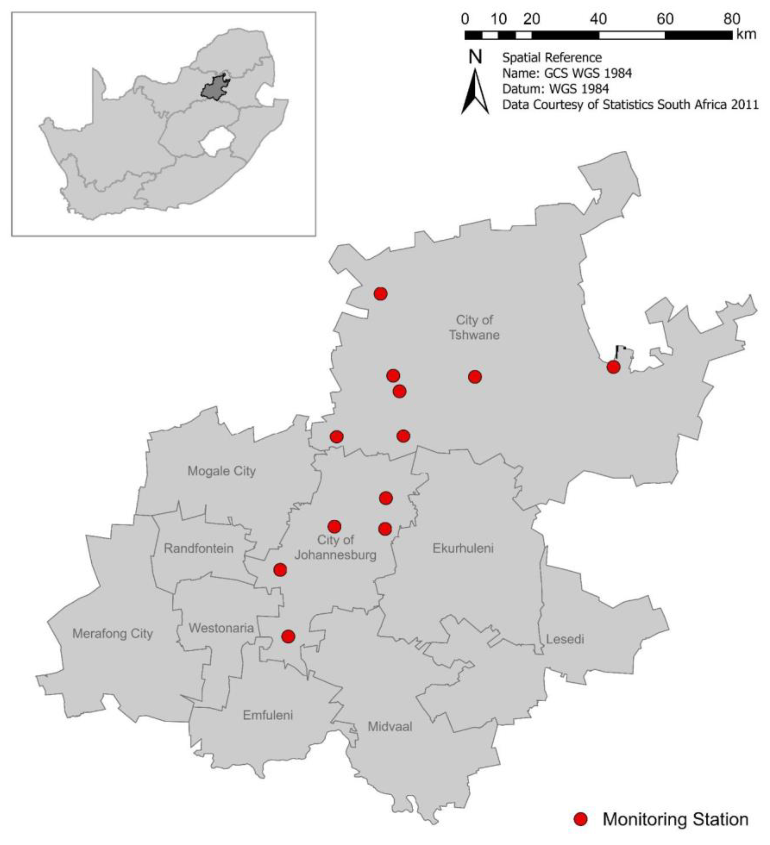
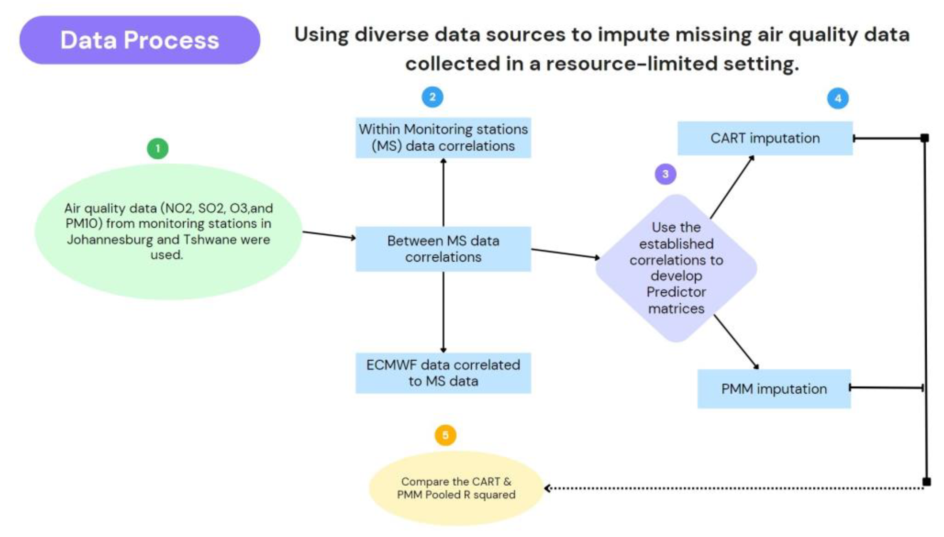
2. Materials and Methods

The current study used ambient air quality data from the cities of Johannesburg and Tshwane. The study period was from 2010 to 2017. Data were obtained from the South African Air Quality Information System (SAAQIS), developed by the Department of Environmental Affairs (DoEA). SAAQIS is the data custodian of the DoEA. The air quality data collected were nitrogen dioxide (NO2), sulfur dioxide (SO2), ozone (O3), and particulate matter less than 10 microns (PM10). Nitric oxide (NO) and carbon monoxide (CO) were other pollutants measured by the monitoring station in the study area. However, the data were not always available and not all the monitoring stations measured NO and CO. Therefore, although the two pollutants are also very important urban pollutants, they were not included in the current study. Figure 5 shows the monitoring stations used in the current study.
The names of the monitoring stations and cities are abbreviated in the figures. The Boding station is abbreviated BG, the Buccleuch station is abbreviated BH, the Booysens station is abbreviated BS, the Olievenhoutbosch station is abbreviated OH, the Mamelodi station is abbreviated MI, the Rosslyn station is abbreviated RN, the Ekandustria station is abbreviated EA, the Newtown station is abbreviated NN, and the Tshwane West station is abbreviated PT. Pta means Pretoria, also known as Tshwane. Jhb means Johannesburg.
Data were shared as hourly averages during the study period, although they were recorded at a finer resolution. Sets of monthly averaged data were also received. Data recorded in parts per billion (ppb) and parts per million (ppm) units were converted to SI units, in micrograms per cubic liter (µg/m3).
The pre-processing and cleaning of the data included testing for outliers (using box and whisker plots), checking data skewness (applying the Shapiro–Wilk test), and testing for any autocorrelations using the variable inflation factor (VIF) method. It is important to test the normality of the data to establish if the log transformation and exponentiation are necessary steps. Extreme values that represented known incidents of equipment calibration were removed. No other assumptions, such as noise, were made about extreme values in the data. It was assumed that these points might have represented actual high exposure (“novelty”) [11].
After removing obvious outliers (for example, an ambient temperature of 100 °C) and converting the recorded parameters to SI units, the date format was changed, and daily average exposures were computed. Scatter plots were used to establish any patterns in the data. This exploration demonstrated the seasonality of the data and further assisted in inspecting the patterns of incompleteness in the data visually. Figure 6 reflects the data process used in the study. In Step 1, data were received from the DoEA. Data were evaluated for incompleteness after all data pre-processing, as discussed. Only monitoring stations with data incompleteness not more than 80% were included in the analysis. Therefore, monitoring stations such as Delta Park and Alexandra were excluded. In Step 2, correlations within and between data from different monitoring stations and the ECMWF sourced data were tested. Once correlations were established, the resultant imputation predictor matrices were developed. These predictor matrices were fed into a CART or PMM MICE imputation algorithm, in statistical software R (Version 4.2.2 (2022-10-31 ucrt)).
Before imputing values, satellite data from the European Centre for Medium Range Weather Forecasts (ECMWF) were downloaded for the two study areas. The downloaded ECMWF data parameters included (1) temperature 2 m above the surface (T2m), (2) boundary layer height (blh), (3) wind speed (ws), (4) total precipitation (tp), and (5) wind direction (wd).
ECMWF utilizes an atmospheric model and data assimilation system which is called the Integrated Forecasting System (IFS) [12]. The structure of the IFS algorithm processes the data in a cyclic approach broadly represented by two computational processes: (a) grid point computations and (b) spectral calculations [12]. The methodology has been adequately published in scientific journals and has been revised and iterated over the years [13]. Forecasting requires that the data be fed into a numerical weather estimation (NWP) model [13]. ECMWF has various data processes (e.g., forecasting and reanalysis) and supports member states with varying capacities of weather forecasting, including the estimation of adverse weather incidents. The aspect of ECMWF data used in the current study related to the phenomenon of data reanalysis as developed, tested, and validated by ECMWF [13]. ECMWF provides data on current forecasts, and reanalyzes climate data sets. These data sets are available on the web, in point-to-point dissemination, in data servers, and in broadcasting. Surface reanalysis data sets from 1 January 2010 to 31 December 2017 were used. The data download followed a three-step approach every six hours starting at midnight.
The current study used MICE to impute the missing data. The MICE package uses predictive correlation matrices to select variables that can be used to estimate missing values in other variables. Therefore, to establish initial predictor matrices, correlations were performed between complete data from the ECMWF and air quality data from the monitoring stations. Correlations of 0.2 and less led to the elimination of a predictor from the predictor matrix. Equally, an anticorrelation led to the exclusion of the predictor variable from the predictor matrix. Various regression or classification techniques can be used to perform MICE, but classification and regression trees (CART) analysis and predictive mean matching methods were used in the current study.
CART was chosen because the algorithm can keep the range of estimated values in a positive range between 0 and the observed maximum value. PMM typically works by selecting a data point from the observed data that has an estimated value close to the estimated value of the missing sample [14]. In certain disciplines of research, constraining data within a specific range may produce an unwanted bias. In such research, multiple imputations are allowed and are believed to achieve better processing estimations when values outside the range are allowed [14].

3. Results

The results are here discussed, initially focusing on the data before the imputations were performed, followed by the results after the imputations. Air quality data from the local monitoring stations were compared with the ECMWF reanalyzed data and correlated to identify relations that were useful for multiple imputations.

3.1. Correlation Studies

Within air quality monitoring stations, correlations between parameters were tested. Correlations were further tested between monitoring stations and further using ECMWF data. Table 1, Table 2 and Table 3 show the correlations of NO2, SO2, O3, and PM10, (a) with other pollutants within a specific station, (b) with the same pollutant at another station, and (c) the correlations of these pollutants with the ECMWF data.
NO2 in the monitoring stations of Olievenhoutbosch, Ekandustria, and Mamelodi had a very strong significance within station correlations with NO.
Some stations did not monitor all the parameters of interest or had no data, i.e., as shown in Table 2, the Ekandustria monitoring station had no PM10 and O3 data. Table 3 shows that the Newtown monitoring station also did not have SO2 data.
The predictor matrices were specified in the CART MICE imputation, where 20 imputed data sets were performed in 10 iterative processes.

3.2. MICE Imputation Algorithm

The predictive ability of pollutants at one monitoring station was varied at other monitoring stations. It was possible to have a prediction matrix which indicated NO2 at one monitoring station predict NO2 at the other monitoring stations. This was however not true for all stations, as was also reflected by the anticorrelations in Table 1, Table 2 and Table 3. The same result was found for SO2, O3, and PM10. ECMWF parameters were found to have mild correlations to varying degrees with NO2, SO2, and PM10 at the monitoring stations in both Johannesburg and Tshwane. Where the correlation coefficients were less than 0.18, the correlation was taken to be very low, or no correlation existed, and the parameters were excluded in the imputation predictor matrix.
Nine different NO2 models, eight SO2 models, eight O3 models, and eight PM10 models were developed. Furthermore, a combined NO2 model was developed using the NO2 data sets of the nine monitoring stations. Similarly, a combined SO2 model and a combined PM10 model based on the nine monitoring stations were also developed. Finally, a composite model was developed using all NO2, SO2, O3, and PM10 data sets.
The regression using both the CART and PMM algorithms estimated the missing values for NO2, SO2, O3, and PM10 at all monitoring stations in both the cities of Johannesburg and Tshwane. The predicted point estimates were mean values. At the end of the computations, there were no missing values. It was found that the range of estimated values fit well with the range of observed values. The mean estimated NO2 ranged from 21.55 µg/m3 to 54.64 µg/m3, estimated SO2 means ranged between 11.17 µg/m3 and 25.66 µg/m3, and the mean estimated PM10 ranged from 1 µg/m3 to 95.28 µg/m3.

3.3. Post-Imputation Test

To assess the quality of the imputation performed, linear regression models using the imputed k data sets were performed and the R-squared statistics of the models were pooled. Table 4 shows the pooled results of the imputed data sets using the CART method and Table 5 reflects the results of the PMM method. The results shown are for pollutants under study at every station and the combined station data for the same pollutants.
The PMM results (Table 5) showed a reduced ability to predict missing data. This result was represented by lower values of the pooled R2 statistics compared to those found when using CART.
The pooled R-squared results of the linear regression model from the imputation performed using CART for all data sets were 0.47 (0.38–0.56), compared to 0.32 (0.30–0.35) for PMM.

4. Discussion

The main objective of this study was to use the MICE algorithms (CART and PMM) to impute incomplete air quality data. The data sets had observations missing completely at random. Data sets for monitoring stations that had missing data with incompleteness over 80% showed considerable differences in correlation tests pre- and post-imputation. These monitoring stations showing greater incompleteness (more than 80%) were excluded. The Alexandra and Delta Park monitoring stations had more than 80% missing data and the post-imputation tests using correlations showed a significant difference between the pre- and post-imputation data correlations.

4.1. Correlation Studies

Although the aim was to impute NO2, SO2, O3, and PM10 data sets, other pollutants received in the data from the monitoring stations were useful. It was important to test the correlations with additional parameters (such as ambient temperature, ozone, and relative humidity measured at a monitoring station) to also establish if they could be useful for the imputation process. Consequently, it was found that O3 at monitoring stations had a moderate positive correlation with the wind speed measured at the monitoring station, but it had a mild positive correlation with the wind speed extracted from the ECMWF data. The two observed correlations were similar. The correlation of ECMWF data might be lower than that measured at the monitoring station due to geographical differences. ECMWF data were downloaded for the Greater Johannesburg and Tshwane metropolises, while the monitoring station data were collected at specific geographic points. Ozone also generally showed a positive correlation with ECMWF T2m and blh. The effects of blh, mixing layer height, and their importance in determining atmospheric pollution have been adequately discussed in the literature [15]. The planetary boundary layer was shown to be correlated with O3 concentration levels in the current study. These observed and reported correlations allowed the researchers to use the available reanalyzed ECMWF blh to compute multiple imputations by chain equations using the CART decision trees regression method.
Ozone also showed negative correlations with SO2 and humidity measured at the monitoring stations. Although NOx species, NO2 in particular, are understood to be the main precursor for the production of O3, the correlation between NO2 and O3 was not stronger than that between O3 and SO2 [16]. These correlations, however, were useful to develop an estimation matrix for computing multiple imputations on the missing data.
NO2 measured at various monitoring stations also showed correlations with ECMWF data. T2m and wind speed from ECMWF data both had a negative correlation with NO2, except at Buccleuch. However, NO2 showed a positive correlation with NO and PM10 measured at the monitoring stations. SO2 and PM10 also showed correlations with ECMWF data and within monitoring station data.
All the above-discussed correlations of available data from monitoring stations, and reanalyzed data extracted from ECMWF data, allowed for successful imputation of the data collected from the Gauteng monitoring stations in the current study. The observed correlations allowed the researchers to develop the predictor matrices. Due to the knowledge of the correlation as observed in the study, it was possible to decide which predictors to silence in the predictor matrix before running the MICE algorithm. This approach of studying correlations before developing a final predictor matrix was greatly useful to allow the inclusion of variables only shown to have a correlation with variables to which the estimators were correlated. Also observed was that the performance of the imputation models improved greatly with the inclusion of ECMWF data. All pooled R2 statistics increased generally by more than 10% when the predictor matrices included ECMWF data.

4.2. MICE Imputation Algorithm

Our predictor matrix showed that NO2 was predictive and could be used as shown by the imputation of missing SO2 and PM10. ECMWF blh, wd, and T2m were observed to be significant predictors of NO2 (in the city), SO2, and PM10 at specific stations. The closer the geographic location of the monitoring station was to the ECMWF geographic point, the greater the estimative power of the ECMWF parameters on the missing data of the monitoring station data. For example, although blh in Tshwane could estimate NO2 in Newtown and Johannesburg, T2m in Tshwane was not predictive of NO2 in Newtown. NO2, SO2, O3, and PM10 could be used to estimate missing values for one another. The predictive relationship may be due to the photochemical relationship of these pollutants [16,17,18]. Furthermore, the plausibility of the correlation between the pollutants, i.e., NO2 and PM10, can be explained by possible common sources such as emissions from vehicles in urban centres [19]. This impact of traffic density in urban areas was also reported in a German study. The study established pollution hotspots (NO2 and PM10 pollution) due to traffic density in three regions (Herne, Oberhausen, and Bochum had high NO2 from vehicle emission, while Herne, Oberhausen, and Gelsenkirchen also had high PM10 from vehicles) [19].
The CART method in MICE imputation produced highly plausible estimated means. The estimated values fell within the restricted range and had no negative values. The use of sequential trees has been preferred and has been shown to produce more plausible and reliable inferences in epidemiology [20]. In fact, CART in MICE has been called ideal [20]. The estimation of NO2 produced models with better pooled R2 statistics than SO2, O3, and PM10.
Although the current study showed successful imputation of air quality data using CART and PMM in a MICE package, the use of real-time measurements, particularly in urban areas with land use and anthropogenic activities known to increase emissions, is recommended. This approach has been shown to be a promising approach and may be more useful for developing countries [21]. Furthermore, future studies can explore the use of other machine learning algorithms such as random forests. The use of low-cost sensors has been proposed for the African context, and the potential use of this cheaper option has been supported [22]. Amegah presents a critical discourse on the possible use of low-cost sensors to enhance and augment the availability of air quality data in sub-Saharan Africa [23]. The current study demonstrates that there is a need to explore these types of sensors. This study recommends that a follow-up study run a pilot test of these types of sensors in the current study setting.

4.3. Post-Imputation Test

The data sets that were imputed were continuous variables. Although the classification and regression trees technique was employed, the regression model that tested the efficacy of MICE in estimating the missing values followed was a linear regression model [24]. Therefore, to test the performance of the imputation results, a combined and fitted linear regression model was performed. Significant model coefficients were observed. Pollutants that were predetermined to be estimative of each other were significant in the data-imputing regression model. The regression models estimated means in place of missing values. This is consistent with other studies [20]. Misconceptions about the veracity of MICE in imputing missing data have been argued by some scholars, and yet the same misconceptions have been addressed in the literature [24]. Some scholars have argued that predictors that have missing data may not be used to estimate and impute missing values for other variables. However, such a use of variables with incompleteness itself to run estimations in imputation methods has been found to be beneficial [24].
Individual pollutant imputation models performed for each monitoring station produced varying estimation performance levels. Using CART, five of the nine stations with NO2 imputations performed had a pooled R2 statistic ranging from 58% to 73%. This post-imputation performance for NO2 was better than both SO2 and PM10. The composite SO2 and PM10 imputation models yielded a pooled R2 statistic of well over 40%. This pooled R2 statistic of 40% is viewed as moderate, which at present is reasonably good [25]. Although other significance test methods are possible to test the performance of imputation estimations, the pooled R-squared statistic has been reported as the preferred method in recent studies [26].

5. Conclusions

The use of correlated air quality data, both from monitoring stations and reanalyzed data from ECMWF, proved useful for the imputation of missing air quality data. Correlation testing was concluded to be a critical step in determining and developing predictor matrices and selecting a variable to include in the regression models of MICE imputation algorithms. The CART method was more predictive and produced more plausible data than PMM. The current study concluded that although air quality data in developing countries settings may be greatly missing, missing at random, or completely at random, it is scientifically possible to utilize platforms like the MICE package to run algorithms such as CART and PMM to estimate and impute missing data. When performed correctly, multiple imputation of air quality data can produce reliable data sets. This was also shown in the Chilean study, concluding that the data imputation yielded better results when covariates from a second monitoring station in Temuco were used. These imputed data sets can reliably be used to make inferences in general epidemiology and computational epidemiological studies. The findings of a successful MICE imputation algorithm (CART) that completes air quality data suggest that more research can be done successfully even when data are considered too absent.

Author Contributions

All authors were involved in the conceptualization of the study, data management, and analysis, and contributed to the write-up. All authors have read and agreed to the published version of the manuscript.

Funding

This research received funding from the South African Medical Research Council: Grant KBLP023-001.407.

Institutional Review Board Statement

Not applicable.

Informed Consent Statement

Not applicable.

Data Availability Statement

Environmental data were available through the municipal offices of the cities and can be requested. The disclosure on the use of the data is a requirement of the cities. Data can be requested on behalf of cities from the Department of Environmental Affairs (DoEA). The data custodian for the DoEA is the South African Air Quality Services (SAAQS), and data can be requested through the SAAQS website using the following website link: Saaqis (environment.gov.za (accessed on 23 September 2022)).

Acknowledgments

The cities of Tshwane and Johannesburg, through the South African Air Quality Information System, provided the air quality data and GIS data used. The data were requested through the SAAQIS website and received from the data custodians.

Conflicts of Interest

The authors declare that they have no conflicts of interest.

References

  1. Prüss-Üstün, A.; Wolf, J.; Corvalán, C.; Bos, R.; Neira, M. Preventing Disease through Healthy Environments: A Global Assessment of the Burden of Disease from Environmental Risks, 2nd ed.; World Health Organization: Geneva, Switzerland, 2016. [Google Scholar]
  2. World Health Organization; Convention on Biological Diversity; United Nations Environment Programme. Connecting Global Priorities: Biodiversity and Human Health: A State of Knowledge Review; UNEP: Geneva, Switzerland, 2015; Available online: http://apps.who.int/iris/bitstream/10665/174012/1/9789241508537_eng.pdf?ua=1 (accessed on 23 September 2022).
  3. World Health Organization. Air Quality Guidelines: Global Update 2005. Particulate Matter, Ozone, Nitrogen Dioxide and Sulfur Dioxide; World Health Organization: Geneva, Switzerland, 2006; Available online: http://www.myilibrary.com?id=95342 (accessed on 23 September 2022).
  4. World Health Organization. Air Quality Criteria and Guides for Urban Pollutants; World Health Organization: Geneva, Switzerland, 1972. [Google Scholar]
  5. World Health Organization; Regional Office for Europe. Effects of Air Pollutants on Human Health: Air Quality Guidelines; UN: Geneva, Switzerland, 1987. [Google Scholar]
  6. Shaw, D.J. Working with Air Quality: A Commentary on the National Environmental Management: Air Quality Act; LexisNexis: Durban, South Africa, 2012. [Google Scholar]
  7. Roda, C.; Nicolis, I.; Momas, I.; Guihenneuc, C. New insights into handling missing values in environmental epidemiological studies. PLoS ONE 2014, 9, e104254. [Google Scholar] [CrossRef] [PubMed]
  8. Quinteros, M.E.; Lu, S.; Blazquez, C.; Cárdenas-R, J.P.; Ossa, X.; Delgado-Saborit, J.-M.; Harrison, R.M.; Ruiz-Rudolph, P. Use of data imputation tools to reconstruct incomplete air quality datasets: A case-study in Temuco, Chile. Atmos. Environ. 2019, 200, 40–49. [Google Scholar] [CrossRef]
  9. White, I.R.; Royston, P.; Wood, A.M. Multiple imputation using chained equations: Issues and guidance for practice. Stat. Med. 2011, 30, 377–399. [Google Scholar] [CrossRef] [PubMed]
  10. Khan, S.I.; Hoque, A.S.M.L. SICE: An improved missing data imputation technique. J. Big Data 2020, 7, 37. [Google Scholar] [CrossRef]
  11. Martínez, J.; Saavedra, Á.; García-Nieto, P.J.; Piñeiro, J.I.; Iglesias, C.; Taboada, J.; Sancho, J.; Pastor, J. Air quality parameters outliers detection using functional data analysis in the Langreo urban area (Northern Spain). Appl. Math. Comput. 2014, 241, 1–10. [Google Scholar] [CrossRef]
  12. ECMWF. Part VI: Technical and computatinal procedures. In Ifs Documentation cy47r1; ECMWF: Reading, UK, 2020. [Google Scholar]
  13. Dee, D.P.; Uppala, S.M.; Simmons, A.J.; Berrisford, P.; Poli, P.; Kobayashi, S.; Andrae, U.; Balmaseda, M.A.; Balsamo, G.; Bauer, P.; et al. The ERA-Interim reanalysis: Configuration and performance of the data assimilation system. Q. J. R. Meteorol. Soc. 2011, 137, 553–597. [Google Scholar] [CrossRef]
  14. Rodwell, L.; Lee, K.J.; Romaniuk, H.; Carlin, J.B. Comparison of methods for imputing limited-range variables: A simulation study. BMC Med. Res. Methodol. 2014, 14, 57. [Google Scholar] [CrossRef]
  15. Yassin, M.; Al-Shatti, L.; A-Rashidi, M. Assessment of the atmospheric mixing layer height and its effects on pollutant dispersion. Environ. Monit. Assess. 2018, 190, 372. [Google Scholar] [CrossRef]
  16. Jhun, I.; Coull, B.A.; Zanobetti, A.; Koutrakis, P. The impact of nitrogen oxides concentration decreases on ozone trends in the USA. Air Qual. Atmos. Health 2014, 8, 283–292. [Google Scholar] [CrossRef] [PubMed]
  17. Demuzere, M.; Trigo, R.M.; Vila-Guerau De Arellano, J.; Van Lipzig, N.P.M. The impact of weather and atmospheric circulation on O3 and PM10 levels at a rural mid-latitude site. Atmos. Chem. Phys. 2009, 9, 2695–2714. [Google Scholar] [CrossRef]
  18. Ngarambe, J.; Joen, S.J.; Han, C.-H.; Yun, G.Y. Exploring the relationship between particulate matter, CO, SO2, NO2, O3 and urban heat island in Seoul, Korea. J. Hazard. Mater. 2021, 403, 123615. [Google Scholar] [CrossRef] [PubMed]
  19. Breuer, J.L.; Samsun, R.C.; Peters, R.; Stolten, D. The impact of diesel vehicles on NOx and PM10 emissions from road transport in urban morphological zones: A case study in North Rhine-Westphalia, Germany. Sci. Total Environ. 2020, 727, 138583. [Google Scholar] [CrossRef] [PubMed]
  20. Burgette, L.F.; Reiter, J.P. Multiple imputation for missing data via sequential regression trees. Am. J. Epidemiol. 2010, 172, 1070–1076. [Google Scholar] [CrossRef] [PubMed]
  21. Lotrecchiano, N.; Sofia, D.; Giuliano, A.; Barletta, D.; Poletto, M. Real-time on-road monitoring network of air quality. Chem. Eng. Trans. 2019, 74, 241. [Google Scholar] [CrossRef]
  22. Sofia, D.; Giuliano, A.; Gioiella, F.; Barletta, D.; Poletto, M. Modeling of an air quality monitoring network with high space-time resolution. In Computer Aided Chemical Engineering; Friedl, A., Klemeš, J.J., Radl, S., Varbanov, P.S., Wallek, T., Eds.; Elsevier: Amsterdam, The Netherlands, 2018; pp. 193–198. [Google Scholar]
  23. Amegah, A.K. Proliferation of low-cost sensors. What prospects for air pollution epidemiologic research in sub-Saharan Africa? Environ. Pollut. 2018, 241, 1132–1137. [Google Scholar] [CrossRef] [PubMed]
  24. Van Ginkel, J.R.; Linting, M.; Rippe, R.C.A.; Van Der Voort, A. Rebutting existing misconceptions about multiple imputation as a method for handling missing data. J. Personal. Assess. 2020, 102, 297–308. [Google Scholar] [CrossRef] [PubMed]
  25. Sarstedt, M.; Ringle, C.M.; Hair, J.F. Partial least squares structural equation modeling. In Handbook of Market Research; Homburg, C., Klarmann, M., Vomberg, A., Eds.; Springer International Publishing: Cham, Switzerland, 2017; pp. 1–40. [Google Scholar]
  26. Van Ginkel, J.R. Significance tests and estimates for r2 for multiple regression in multiply imputed datasets: A cautionary note on earlier findings, and alternative solutions. Multivar. Behav. Res. 2019, 54, 514–529. [Google Scholar] [CrossRef] [PubMed]
Figure 1. Data overlap and patterns of missing data for NO2 compared for nine monitoring stations.
Atmosphere 15 00303 g001
Figure 2. Data overlap and patterns of missing data for SO2 compared for eight monitoring stations.
Atmosphere 15 00303 g002
Figure 3. Data overlap and patterns of missing data for PM10 compared for eight monitoring stations.
Atmosphere 15 00303 g003
Figure 4. Data overlap and patterns of missing data for O3 compared for eight monitoring stations.
Atmosphere 15 00303 g004
Figure 5. Air quality monitoring stations in the cities of Johannesburg and Tshwane.
Atmosphere 15 00303 g005
Figure 6. A flow diagram of the study data process.
Atmosphere 15 00303 g006
Table 1. The predictor matrices of NO2, SO2, O3, and PM10 in the air quality data of the Bodibeng, Buccleuch, and Booysens stations.
NO2SO2PM10O3
BodibengWithin stationNO (r = 0.75)PM10 (r = 0.42)Humidity (r = −0.51)Wind speed (r = 0.34)
CO (r = 0.58)NO (r = 0.25)NO2 (r = 0.61)Temperature (r = 0.32)
PM10 (r = 0.61) NO (r = 0.70)
Between stationsTshwane west NO2 (r = 0.62)Ekandustria SO2 (r = 0.63)Tshwane west PM10 (r = 0.72)Buccleuch O3 (r = 0.45)
Rosslyn NO2 (r = 0.47)Rosslyn SO2 (r = 0.53)Rosslyn PM10 (r = 0.50)Booysens O3 (r = 0.54)
Olievenhoutbosch NO2 (r = 0.37)Mamelodi SO2 (r = 0.25)Mamelodi PM10 (r = 0.16)Mamelodi O3 (r = 0.64)
Newtown NO2 (r = 0.53)Booysens SO2 (r = 0.43)Booysens PM10 (r = 0.63)Rosslyn O3 (r = 0.64)
Booysens NO2 (r = 0.44)Tshwane west SO2 (r = 0.34)Olievenhoutbosch PM10 (r = 0.59)Olievenhoutbosch O3 (r = 0.64)
Mamelodi NO2 (r = 0.39)Olievenhoutbosch SO2 (r = 0.33)Buccleuch PM10 (r = 0.56)Newtown O3 (r = 0.13)
Buccleuch NO2 (r = −0.40)Buccleuch SO2 (r = −0.13)Newtown PM10 (r = 0.56)
Ekandustria NO2 (r = 0.12)
ECMWFTshwane wind direction (r = −0.27)Tshwane total precipitation (r = −0.15)Tshwane total precipitation (r = −0.22)Tshwane temperature @2m (r = 0.31)
Tshwane temperature @2m (r = −0.12) Tshwane temperature @2m (r = −0.22)Tshwane blh (r = 0.25)
Tshwane total precipitation (r = −0.16)
BuccleuchWithin stationNO (r = 0.36)Humidity (r = −0.51)NO (r = 0.39)Wind speed (r = −0.15)
Ambient temperature (r = 0.23)PM10 (r = 0.27)SO2 (r = 0.27)SO2 (r = −0.27)
SO2 (r = 0.15)03 (r = −0.28) Humidity (r = −0.15)
Between stationsNewtown NO2 (r = −0.65)Olievenhoutbosch SO2 (r = 0.63)Bodibeng PM10 (r = 0.56)Bodibeng O3 (r = 0.45)
Olievenhoutbosch NO2 (r = −0.48)Ekandustria SO2 (r = 0.67)Tshwane west PM10 (r = 0.50)Mamelodi O3 (r = 0.27)
Tshwane west NO2 (r = −0.38)Mamelodi SO2 (r = 0.37)Mamelodi PM10 (r = 0.44)Tshwane west O3 (r = 0.21)
Bodibeng NO2 (r = −0.40)Rosslyn SO2 (r = 0.30)Booysens PM10 (r = 0.24)Olievenhoutbosch O3 (r = 0.16)
Ekandustria NO2 (r = −0.23)Bodibeng SO2 (r = −0.13)Olievenhoutbosch PM10 (r = 0.33)
Booysens NO2 (r = 0.10)Booysens SO2 (r = 0.043)Rosslyn PM10 (r = 0.29)
Newtown PM10 (r = 0.57)
ECMWFJohannesburg temperature @2m (r = 0.29)Johannesburg total precipitation (r = −0.20)Johannesburg wind speed (r = 0.14)
Johannesburg blh (r = 0.18)Johannesburg temperature @2m (r = −0.15)
BooysensWithin stationNO (r = 0.37)03 (r = −0.36)NO (r = 0.56)Wind speed (r = 0.36)
Ambient temperature (r = −0.46)NO (r = 0.28)Ambient temperature (r = −0.42)Temperature (r = 0.25)
PM10 (r = 0.28) NO2 (r = 0.28)
Wind speed (r = −0.33)
Between stationsRosslyn NO2 (r = 0.64)Olievenhoutbosch SO2 (r = 0.47)Olievenhoutbosch PM10 (r = 0.65)Bodibeng O3 (r = 0.64)
Newtown NO2 (r = 0.62)Mamelodi SO2 (r = 0.42)Bodibeng PM10 (r = 0.63)Mamelodi O3 (r = 0.75)
Olievenhoutbosch NO2 (r = 0.49)Rosslyn SO2 (r = 0.42)Buccleuch PM10 (r = 0.24)Olievenhoutbosch O3 (r = 0.55)
Mamelodi NO2 (r = 0.44)Bodibeng SO2 (r = 0.43)Tshwane west PM10 (r = 0.21)Tshwane west O3 (r = 0.79)
Bodibeng NO2 (r = 0.44)Ekandustria SO2 (r = 0.35)Rosslyn PM10 (r = 0.14)Rosslyn O3 (r = 0.41)
Ekandustria NO2 (r = 0.28) Newtown PM10 (r = 0.58)
Buccleuch NO2 (r = 0.10)Buccleuch SO2 (r = 0.043)Mamelodi PM10 (r = 0.008)
ECMWFTshwane total precipitation (r = −0.16)Tshwane temperature @2m (r = −0.11)Tshwane wind direction (r = −0.15)Tshwane temperature @2m (r = 0.27)
Tshwane temperature @2m (r = −0.22)Tshwane wind speed (r = −0.12)Tshwane total precipitation (r = −0.13)Tshwane blh (r = 0.21)
Tshwane wind direction (r = 0.13)
Table 2. The predictor matrices of NO2, SO2, O3, and PM10 in the air quality data of the Olievenhoutbosch, Ekandustria, and Mamelodi stations.
NO2SO2PM10O3
OlievenhoutboschWithin stationNO (r = 0.77)NO2 (r = 0.31)NO2 (r = 0.62)Wind speed (r = 0.28)
CO (r = 0.57)CO (r = 0.29)CO (r = 0.52)Temperature (r = 0.23)
PM10 (r = 0.62)PM10 (r = 0.24)NO (r = 0.50)
Between stationsMamelodi NO2 (r = 0.71)Mamelodi SO2 (r = 0.52)Bodibeng PM10 (r = 0.59)Bodibeng O3 (r = 0.64)
Rosslyn NO2 (r = 0.62)Buccleuch SO2 (r = 0.63)Booysens PM10 (r = 0.65)Mamelodi O3 (r = 0.66)
Tshwane west NO2 (r = 0.47)Ekandustria SO2 (r = 0.55)Newtown PM10 (r = 0.52)Booysens O3 (r = 0.55)
Booysens NO2 (r = 0.49)Booysens SO2 (r = 0.47)Mamelodi PM10 (r = 0.18)Tshwane west O3 (r = 0.37)
Buccleuch NO2 (r = −0.48)Bodibeng SO2 (r = 0.33)Tshwane west PM10 (r = 0.32)Rosslyn O3 (r = 0.63)
Newtown NO2 (r = 0.46)Rosslyn SO2 (r = 0.44)Rosslyn PM10 (r = 0.32)
Bodibeng NO2 (r = 0.37) Buccleuch PM10 (r = 0.52)
ECMWFTshwane wind speed (r = −0.21)Tshwane wind direction (r = 0.23)Tshwane total precipitation (r = −0.21)Tshwane temperature @2m (r = 0.28)
Tshwane temperature @2m (r = −0.26)Tshwane wind speed (r = −0.18)Tshwane temperature @2m (r = −0.20)Tshwane blh (r = 0.23)
Tshwane total precipitation (r = −0.16)
EkandustriaWithin stationNO (r = 0.82)Wind speed (r = −0.16)
Between stationsMamelodi NO2 (r = 0.34)Bodibeng SO2 (r = 0.63)
Rosslyn NO2 (r = −0.28)Rosslyn SO2 (r = 0.56)
Booysens NO2 (r = −0.28)Olievenhoutbosch SO2 (r = 0.55)
Bodibeng NO2 (r = 0.12)Buccleuch SO2 (r = 0.67)
Booysens SO2 (r = 0.35)
Mamelodi SO2 (r = 0.26)
ECMWFTshwane wind speed (r = −0.18)Tshwane wind speed (r = −0.31)
Tshwane temperature @2m (r = −0.20)Tshwane wind direction (r = 0.18)
Tshwane temperature @2m (r = −0.13)
MamelodiWithin stationNO (r = 0.87)PM10 (r = −0.27)NO2 (r = 0.31)Wind speed (r = 0.42)
Humidity (r = −0.51)NO2 (r = 0.20)NO (r = 0.36)Temperature (r = 0.31)
PM10 (r = 0.62)Ambient temperature (r = −0.20)SO2 (r = 0.27)PM10 (r = 0.25)
Between stationsRosslyn NO2 (r = 0.71)Olievenhoutbosch SO2 (r = 0.52)Tshwane west PM10 (r = 0.57)Bodibeng O3 (r = 0.64)
Olievenhoutbosch NO2 (r = 0.71)Booysens SO2 (r = 0.42)Rosslyn PM10 (r = 0.73)Booysens O3 (r = 0.75)
Booysens NO2 (r = 0.44)Bodibeng SO2 (r = 0.25)Buccleuch PM10 (r = −0.44)Buccleuch O3 (r = 0.27)
Tshwane west NO2 (r = 0.19)Tshwane west SO2 (r = 0.28)Olievenhoutbosch PM10 (r = 0.18)Newtown O3 (r = 0.33)
Bodibeng NO2 (r = 0.39)Rosslyn SO2 (r = 0.33)Bodibeng PM10 (r = 0.16)Tshwane west O3 (r = 0.24)
Ekandustria NO2 (r = 0.34)Ekandustria SO2 (r = 0.26)Booysens PM10 (r = 0.008)Rosslyn O3 (r = 0.75)
Newtown NO2 (r = −0.15)Buccleuch SO2 (r = 0.37) Olievenhoutbosch O3 (r = 0.66)
ECMWFTshwane temperature @2m (r = −0.11)Tshwane temperature @2m (r = −0.17)Tshwane temperature @2m (r = −0.16)Tshwane temperature @2m (r = 0.34)
Tshwane wind direction (r = 0.18) Tshwane blh (r = 0.23)
Table 3. The predictor matrices of NO2, SO2, O3, and PM10 in the air quality data of the Tshwane West, Rosslyn, and Newtown stations.
NO2SO2PM10O3
Tshwane westWithin stationWind speed (r = −0.57)Wind direction (r = −0.22)NO (r = 0.57)Wind speed (r = 0.49)
NO (r = 0.51)O3 (r = −0.23)NO2 (r = 0.42)Temperature (r = −0.28)
PM10 (r = 0.42) CO (r = 0.70)SO2 (r = −0.23)
Between stationsOlievenhoutbosch NO2 (r = 0.47)Ekandustria SO2 (r = 0.44)Bodibeng PM10 (r = 0.72)Mamelodi O3 (r = 0.24)
Rosslyn NO2 (r = 0.55)Olievenhoutbosch SO2 (r = 0.10)Mamelodi PM10 (r = 0.57)Booysens O3 (r = 0.79)
Bodibeng NO2 (r = 0.62)Mamelodi SO2 (r = 0.28)Newtown PM10 (r = 0.71)Buccleuch O3 (r = 0.27)
Mamelodi NO2 (r = 0.19)Bodibeng SO2 (r = 0.34)Rosslyn PM10 (r = 0.54)Newtown O3 (r = 0.33)
Newtown NO2 (r = 0.42)Rosslyn SO2 (r = 0.24)Buccleuch PM10 (r = 0.50)Olievenhoutbosch O3 (r = 0.37)
Olievenhoutbosch PM10 (r = 0.32)
ECMWFTshwane total precipitation (r = −0.14)Tshwane total wind direction (r = 0.14)Tshwane total precipitation (r = −0.18)Tshwane temperature @2m (r = 0.31)
Tshwane temperature @2m (r = −0.13) Tshwane blh (r = 0.35)
RosslynWithin stationNO (r = 0.81)NO2 (r = 0.47)NO2 (r = 0.55)Wind speed (r = 0.34)
PM10 (r = 0.55)NO (r = 0.45)NO (r = 0.57)Temperature (r = 0.50)
SO2 (r = 0.47) SO2 (r = 0.25)NO (r = −0.41)
Ambient temperature (r = −0.48) NO2 (r = −0.36)
Between stationsMamelodi NO2 (r = 0.71)Ekandustria SO2 (r = 0.56)Bodibeng PM10 (r = 0.50)Mamelodi O3 (r = 0.75)
Olievenhoutbosch NO2 (r = 0.62)Bodibeng SO2 (r = 0.53)Tshwane west PM10 (r = 0.54)Booysens O3 (r = 0.41)
Booysens NO2 (r = 0.64)Booysens SO2 (r = 0.42)Mamelodi PM10 (r = 0.73)Tshwane west O3 (r = 0.56)
Tshwane west NO2 (r = 0.55)Tshwane west SO2 (r = 0.24)Newtown PM10 (r = 0.28)Bodibeng O3 (r = 0.49)
Ekandustria NO2 (r = 0.28)Olievenhoutbosch SO2 (r = 0.44) Buccleuch PM10 (r = 0.29)Olievenhoutbosch O3 (r = 0.63)
Bodibeng NO2 (r = 0.47)Mamelodi SO2 (r = 0.33)Olievenhoutbosch PM10 (r = 0.32)
Newtown NO2 (r = 0.18)Buccleuch SO2 (r = 0.67)Booysens PM10 (r = 0.14)
ECMWFTshwane temperature @2m (r = −0.28)Tshwane temperature @2m (r = −0.12)Tshwane temperature @2m (r = −0.11)Tshwane temperature @2m (r = 0.48)
Tshwane total precipitation (r = −0.15)Tshwane blh (r = 0.39)
NewtownWithin stationWind speed (r = −0.30) NO (r = 0.49)Wind speed (r = 0.23)
Wind speed (r = −0.31)Temperature (r = 0.21)
NO2 (r = 0.28)
Between stationsBuccleuch NO2 (r = −0.65) Tshwane west PM10 (r = 0.71)Mamelodi O3 (r = 0.33)
Booysens NO2 (r = 0.62) Booysens PM10 (r = 0.58)Olievenhoutbosch O3 (r = 0.17)
Bodibeng (r = 0.53) Buccleuch PM10 (r = −0.57)
Tshwane west NO2 (r = 0.42) Rosslyn PM10 (r = −0.28)
Olievenhoutbosch NO2 (r = 0.46) Bodibeng PM10 (r = 0.56)
Rosslyn NO2 (r = 0.18) Olievenhoutbosch PM10 (r = 0.52)
ECMWFJohannesburg blh (r = −0.19) Johannesburg total precipitation (r = −0.13)
Johannesburg Wind speed (r = −0.18)
Table 4. Pooled R-squared estimates using classification and regression trees (CART)-imputed data.
StationNO2SO2PM10O3
Bodibeng0.58 (0.54–0.62)0.50 (0.42–0.57)0.68 (0.65–0.71)0.50 (0.47–0.54)
Buccleuch0.39 (0.28–0.45)0.44 (0.41–0.48)0.45 (0.36–0.53)0.14 (0.01–0.35)
Booysens0.37 (0.29–0.45)0.34 (0.28–0.40)0.48 (0.41–0.54)0.65 (0.61–0.68)
Olievenhoutbosch0.72 (0.66–0.77)0.51 (0.44–0.58)0.45 (0.39–0.52)0.61 (0.55–0.67)
Ekandustria0.73 (0.67–0.78)0.48 (0.43–0.53)
Mamelodi0.63 (0.58–0.68)0.34 (0.28–0.39)0.49 (0.40–0.57)0.64 (0.59–0.69)
Pretoria0.36 (0.28–0.45)0.24 (0.12–0.38)0.52 (0.31–0.69)0.43 (0.31–0.96)
Rosslyn0.77 (0.74–0.79)0.38 (0.32–0.43)0.47 (0.38–0.56)0.66 (0.61–0.72)
Newtown0.36 (0.28–0.45) 0.43 (0.40–0.54)0.33 (0.22–0.44)
All combined0.61 (0.40–0.76)0.48 (0.42–0.54)0.47 (0.39–0.54)0.13 (0.03–0.28)
Table 5. Pooled R-squared estimates using predictive mean matching (PMM)-imputed data.
StationNO2SO2PM10O3
Bodibeng0.57 (0.55–0.59)0.28 (0.25–0.31)0.52 (0.49–0.54)0.31 (0.28–0.34)
Buccleuch0.26 (0.24–0.29)0.26 (0.23–0.29)0.16 (0.13–0.19)0.06 (0.05–0.08)
Booysens0.15 (0.13–0.17)0.11 (0.09–0.13)0.33 (0.30–0.36)0.24 (0.21–0.26)
Olievenhoutbosch0.63 (0.61–0.65)0.26 (0.23–0.29)0.35 (0.32–0.38)0.35 (0.33–0.38)
Ekandustria0.03 (0.02–0.04)0.16 (0.14–0.19)
Mamelodi0.48 (0.45–0.51)0.16 (0.13–0.18)0.13 (0.10–0.15)0.44 (0.41–0.46)
Pretoria0.28 (0.25–0.31)0.05 (0.04–0.07)0.21 (0.18–0.24)0.16 (0.14–0.19)
Rosslyn0.77 (0.74–0.79)0.23 (0.20–0.26)0.36 (0.33–0.39)0.38 (0.35–0.41)
Newtown0.14 (0.12–0.17) 0.25 (0.22–0.28)0.03 (0.02–0.04)
Stations combined0.23 (0.20–0.26)0.25 (0.23–0.28)0.25 (0.23–0.28)0.02 (0.01–0.03)
Disclaimer/Publisher’s Note: The statements, opinions and data contained in all publications are solely those of the individual author(s) and contributor(s) and not of MDPI and/or the editor(s). MDPI and/or the editor(s) disclaim responsibility for any injury to people or property resulting from any ideas, methods, instructions or products referred to in the content.

