Article

NH3 Emissions and Lifetime Estimated by Satellite Observations with Differential Evolution Algorithm

1
School of Advanced Manufacturing Engineering, Hefei University, Hefei 230601, China
2
Key Laboratory of Environmental Optics and Technology, Anhui Institute of Optics and Fine Mechanics, Chinese Academy of Sciences, Hefei 230031, China
*
Author to whom correspondence should be addressed.
Atmosphere 2024, 15(3), 251; https://doi.org/10.3390/atmos15030251
Submission received: 27 December 2023 / Revised: 18 February 2024 / Accepted: 19 February 2024 / Published: 21 February 2024
(This article belongs to the Section Atmospheric Techniques, Instruments, and Modeling)

Abstract

:
As an important irritant trace gas in the atmosphere, ammonia (NH3) significantly impacts human health and environment. Bottom-up emission inventories are widely used to estimate ammonia emissions and their geographical distributions over China. However, high uncertainties are still associated with emission inventories due to inaccurate emission factors used. The Differential Evolution (DE) algorithm is a population-based stochastic optimization algorithm used to solve complicated optimization problems. We quantify NH3 emissions and lifetime from Infrared Atmospheric Sounding Interferometer (IASI) NH3 observations together with MERRA-2 wind fields based on the DE algorithm. Two inland cities, Urumchi and Golmud in China, are chosen to study of the NH3 emissions based on the distributions of NH3 total columns and wind fields. The NH3 emissions rate estimated is about 5.84 × 10⁻¹¹ and 4.19 × 10⁻¹¹ kg·m−2s−1 in Urumchi and in the Golmud area from May to September from 2008 to 2023, respectively. The lifetime of NH3 estimated in the two areas is 4.31 and 9.19 h, respectively. We compare the NH3 emissions and lifetime estimated in this study with the values in other studies, and the results show the reliability of the method used. This work is one of few quantitative studies of NH3 emissions from cities using satellite observations in China.

1. Introduction

Ammonia is a strong irritant gas and can cause respiratory problems when inhaled in high concentrations [1]. An increase in ammonia concentration in the atmosphere have negative effects on human health [2]. It also can cause skin and eye irritation at high concentrations [3]. In addition, atmospheric ammonia can react with other acidifying pollutants to form fine particulate matter, which can lead to respiratory and cardiovascular diseases [4]. Also, long-term exposure to high levels of ammonia can harm the environment, including plants and soil fertility [5]. So, it is important to monitor and control ammonia emissions in order to maintain a healthy and safe environment.
Sources of atmospheric ammonia are agriculture (animal waste, fertilizer application), industry (production of chemicals, manufacturing processes), biomass burning, vehicle exhaust, soils, natural vegetation, wild animals, and oceans. Sinks of atmospheric ammonia include dry deposition, wet removal by precipitation, and conversion to particulate ammonium salts via reaction with acids. Based on the activity data on fertilizer application, livestock farming, fertilizer production, and populations with emission factors of various ammonia sources, bottom-up emission inventories are developed to estimate China’s atmospheric ammonia emissions and its geographical distributions. However, there is large uncertainty in emission estimation due to the inaccurate emission factors used.
Satellite remote sensing has been widely used in estimating gas emissions. With the help of satellite sensors, we can observe the concentration distributions of various gases in the atmosphere, such as sulfur dioxide (SO2), nitrogen dioxide (NO2), Ozone (O3), carbon dioxide (CO2), carbon monoxide (CO), methane (CH4), and ammonia (NH3), etc. [6,7,8,9,10,11,12,13]. Based on the spatial and temporal distribution of gases measured by satellite, emissions can be estimated from various sources, such as industrial plants, vehicles, and agricultural activities [14]. Satellite remote sensing provides a valuable tool for monitoring emissions of pollution gases and greenhouse gases, which is critical for pollution control and mitigating climate change [15,16].
Satellite observations can resolve the emission sources with a higher resolution than the bottom-up inventory methods [17]. Detecting emissions from point source shows a significant advantage for short-lived gases, such as SO2, NO2, and NH3, as the emissions of the point sources can be derived with a simple mass balance method [18,19,20]. Beirle et al. used NO2 tropospheric columns observed by Ozone Monitoring Instrument (OMI) satellite, wind information, and the downwind decay to derive the emissions from megacities and continuously emitting point sources [21]. Liu et al. used the method proposed by Beirle et al. [21] to estimate the emissions of cities and NOx lifetime by the variations of plume with wind speed [22,23,24]. Zhang et al. used SO2 columns observed by OMI and SO2 profiles derived from the MOZART-4 model to evaluate ground-level SO2 concentrations over China [25]. Kourtidis et al. developed a box model that calculates SO2 emissions using relationships between gridded OMI satellite data of NO2 and SO2 with calm wind [26]. The anthropogenic emissions of NO2 and SO2 in China simulated by modeling were compared with the values derived from OMI data and ground level observations [27].
In addition, Zhang et al. used a GEOS-Chem joint model and Tropospheric Emission Spectrometer (TES) satellite NH3 columns to estimate anthropogenic NH3 emissions in China, at the 0.5° × 0.67° horizontal resolution, and the calculated annual NH3 emissions were 22.06 Tg in 2008 [28]. Van Damme et al. used a decade of daily observations from Infrared Atmospheric Sounding Interferometer (IASI) satellite, to produce a high spatial resolution map of global distribution of NH3, and identify the world’s industrial and agricultural ammonia point sources, and the annual growth of NH3 columns over China were about (24.7 ± 2.1) × 1013 molec cm−2 yr−1 from 2008 to 2018 [29]. Clarisse et al. identified the type of global NH3 point sources by a wind-adjusted super resolution method using IASI satellite data [30]. Clarisse et al. found some atmospheric ammonia emanations by an oversampling method using IASI satellite-derived atmospheric NH3 data [31]. Dammers et al. used IASI and Cross-track Infrared Sounder (CrIS) satellite observations to identify large NH3 point sources and estimate their emissions, and the estimated ammonia emissions over China are about 1556 kt yr−1 [32]. Li et al. improved fertilizer-related NH3 emission inventories and derived the atmospheric NH3 emissions in mainland China about 12.11 Tg in 2016 [33].
Previous studies have shown that ammonia has a lifetime of about a few hours to a few days [13]. Van Damme et al. used a box model to identify, categorize and quantify the world’s ammonia emission hotspots based on IASI satellite observations, and the average effective lifetime of ammonia is smaller than 12 h [13]. Dammers et al. used a wind rotation approach, the exponentially modified Gaussian (EMG) method and CrIS and IASI(A and B) satellite data to estimate NH3 emissions and lifetimes from large agricultural and industrial point sources, and the computed NH3 lifetime for large point sources is on average 2.35 ± 1.16 h [32]. Hauglustaine et al. used a global model to summarize the global budget of ammonia and ammonium, and the corresponding simulation lifetime of ammonia in the atmosphere was 15 h in 2000 [34]. Shephard et al. used a 2D exponentially modified Gaussian (EMG) plume model and CrIS satellite data from April to September from 2013 to 2017 to estimate the lifetime of ammonia, and the estimated lifetime was 2.66 h [35]. Abeed et al. used IASI satellite observations, ECMWF and MERRA-2 reanalysis data products, and a GEOS-Chem model to estimate agricultural ammonia volatilization over Europe, and the lifetime is estimated to be about 6 h in Europe [36]. Evangeliou et al. used IASI and CrIS satellite data, a chemistry transport model, and an Inverse distance weighting (IDW) interpolation method to calculate the global ammonia emissions during the period 2008–2017, and the calculated ammonia averaged lifetime is about 11 h [37]. Whitburn et al. used IASI satellite data in the years 2008–2015 and a simple box model to estimate the NH3 emissions over Indonesia, and the derived lifetime of NH3 is between 12 and 36 h [38].
Due to the limitations of the spatial and temporal resolution of satellite observations, it is difficult to accurately estimate emissions from small-scale sources, especially for those non-isolated sources. However, satellite observations can resolve isolated emission sources (no other large sources within 100~200 km radius) and estimate emissions from these sources accurately.
The purpose of this study is to quantify NH3 emissions from several inland cities located in China and estimate the lifetime of atmospheric NH3 based on IASI satellite observations and wind information. Section 2 introduces the data and methods used in this work. Section 3 gives the results and discussion. The NH3 emissions and the lifetime are calculated for two cities during “ozone season” (May–September) from 2008 to 2023. Section 4 makes the conclusions.

2. Materials and Methods

2.1. IASI Data

IASI is a satellite payload designed for atmospheric sounding and climate monitoring. It is operated by the European Organization for the Exploitation of Meteorological Satellites (EUMETSAT) onboard the Metop series of polar-orbiting satellites. The MetOp-A, MetOp-B, and MetOp-C satellite of the series were launched in 2006, 2012, and 2018, respectively.
IASI measures the infrared radiation emitted by the Earth’s atmosphere in the spectral range of 645–2760 cm−1 with a high spectral resolution of 0.25 cm−1. By analyzing the atmospheric radiation, IASI observations can be used to retrieve vertical profiles of temperature and humidity, as well as the concentration of various atmospheric trace gases, including carbon monoxide, ozone, methane, and sulfur dioxide. IASI provides global coverage with a revisit time of less than 12 h, making it a valuable tool for weather forecasting, air quality monitoring, and climate research. IASI measurements have been used to study the trend and variability of atmospheric composition, to evaluate the performance of climate models, and to investigate the impact of human activities on the Earth’s atmosphere [39,40,41,42].
The main source of ammonia emissions comes from the large-scale use of ammonia fertilizers in agriculture [43]. Agriculture is considered the dominant source of atmospheric ammonia and contributes over 81% of global NH3 emissions [29]. “Ozone season” (May to September) is both the high-ozone season and the growing season of animals and plants, when ammonia concentrations are high [44]. NH3 total column data of MetOp-A and MetOp-B over China during “ozone season” (May to September) from 2008 to 2023 are used in this work. The IASI NH3 total columns (v4.0.0, ULB-LATMOS) measured in “cloud free” (cloud fraction below 30%) days are considered. For inter-annual comparisons and trends analyses, this work also uses the reanalyzed daily IASI ammonia (NH3) total column dataset.

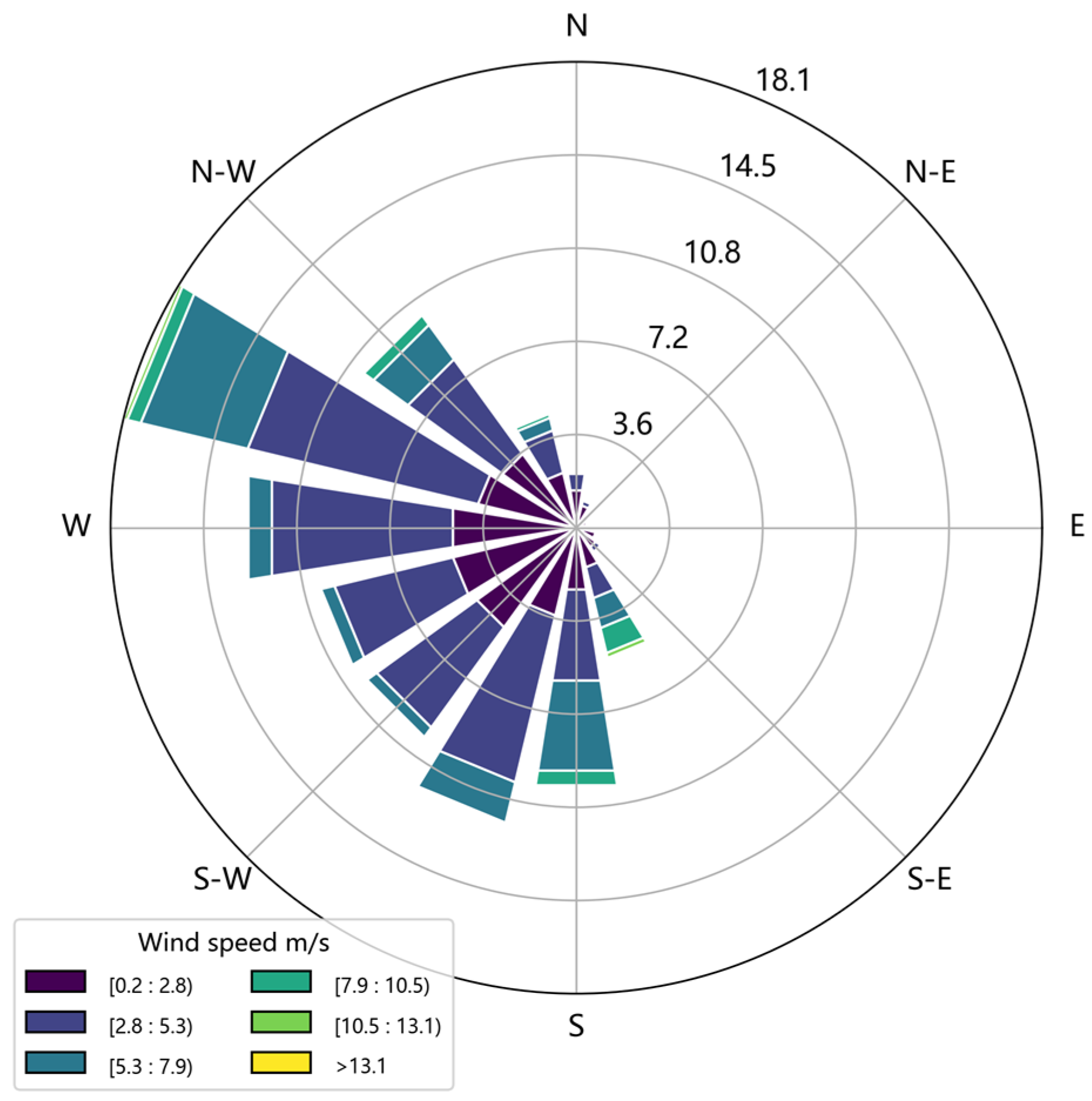
2.2. MERRA-2 Wind Field

Modern-Era Retrospective analysis for Research and Applications (MERRA-2) is a NASA atmospheric reanalysis product [45] which provides long-term, global atmospheric data from 1980 to the present. It is based on the Goddard Earth Observing System Model, Version 5 (GEOS-5), and assimilates a wide range of observations, including satellite, ground-based, and aircraft data.
MERRA-2 includes a wide range of atmospheric parameters, such as temperature, humidity, wind, pressure, precipitation, and aerosol concentrations. It provides hourly, daily, and monthly data at a horizontal resolution of 0.5 degree latitude by 0.625 degree longitude, making it a valuable resource for climate research, weather forecasting, and air quality studies.
In this study, the M2I1NXASM dataset in MERRA-2 was selected with a time resolution of 1 h, downloaded from https://gmao.gsfc.nasa.gov/reanalysis/MERRA-2/ (accessed on 20 February 2024). The U50M and V50M data representing the wind direction are used and linearly interpolated to a grid of 0.01° × 0.01° in this work.

2.3. Emission Estimation

Beirle et al. used wind field information to classify NO2 data by different wind downwards and proposed the “line density” method [21]. This method can effectively avoid the neutralization effect of the opposite wind direction data and help to obtain the dispersion pattern of pollutants clearly. Ammonia, like nitrogen dioxide, is a short-lived gas, so ammonia emissions can be estimated using this method. The “line density” concept was proposed to simplify the two-dimensional problem of the spatial distribution of NH3 concentration to a one-dimensional problem. Integrating the NH3 columns across the respective main wind direction, the two-dimensional mean NH3 columns distribution is reduced to one-dimensional “line densities”.
A simple model function M(x) as a function of the distance x was used to fit the observed NH3 line densities.
M ( x ) = E × ( e G ) ( x ) + B
where E is total NH3 emissions, B is a constant background of NH3, and e(x) is a truncated exponential function:
{ e ( x ) = exp ( ( x X ) / x 0 ) x X e ( x ) = 0 x < X
where X is the location of the emission source relative to a city center, and x0 is the e-folding distance downwind. G(x) is a Gaussian function with standard deviation σ to describe the interference of different factors on the ideal distribution e(x).
G ( x ) = 1 2 π σ exp ( x 2 2 σ 2 )
The parameters, including total emissions E, e-folding distance x0, constant background B, location of the emission source X, and standard deviation σ of G(x), are estimated by the non-linear least-square fit or other algorithms. Least-square fit easily gets stuck in a local minimum, so we used the Differential Evolution optimization algorithm to estimate the parameters in this study.

2.4. Differential Evolution Optimization Algorithm

Differential Evolution (DE) is a stochastic, population-based optimization algorithm belonged to the family of Evolutionary Algorithms. DE was first proposed by Storn and Price [46], and it has been widely used in engineering design, machine learning, and financial modeling to solve some complicated optimization problems, as it is an efficient parallel search algorithm. DE is a population-based stochastic search technique that relies on mutation, crossover, and selection operators at each generation to evolve a collection of candidate solutions toward an optimal state. In this study, NH3 total columns are calculated separately for calm and four different wind direction sectors, for a calm threshold of 2 m/s. For each wind direction sector, line densities are calculated by spatial integration in across-wind direction. So, the mean column distributions (two-dimensional, 2D) are reduced to one-dimensional “line densities” along the respective main wind direction. Then, we use DE algorithm to fit of a simple model function to the observed NH3 line densities in order to determine the parameters (E, x0, B, X, σ) by iteratively adjusting the five parameters to make the calculated line density close to the observed line density. The parameters include NH3 emissions, and the lifetime (τ = x0/w) of NH3 is derived from the mean wind w and e-folding distance x0, where w is the projected mean wind speed on the main wind direction. The basic idea behind DE is to maintain a population of candidate solutions and evolve them iteratively by applying three main operations: mutation, crossover, and selection. At each iteration, a new population is created by applying the mutation operation to the current population. The ith individual vector X i , G of the population in generation G has D components.
X i , G = [ x 1 , i , G , x 2 , i , G , x 3 , i , G , , x D , i , G ]
This involves generating a mutant vector V i , G by adding a scaled difference vector between two randomly chosen population vectors to a third population vector.
V i , G = X r 1 i , G + F ( X r 2 i , G X r 3 i , G )
The crossover operation is used to combine the V i , G with a randomly selected population vector. Then, produce a trial vector U i , G .
U i , G = [ u 1 , i , G , u 2 , i , G , u 3 , i , G , , u D , i , G ]
u j , i , G = { v j , i , G i f ( r a n d i , j [ 0 , 1 ] C r o r j = j r a n d ) x j , i , G o t h e r w i s e
Finally, the selection operation is used to choose between the U i , G and the corresponding original vector for the next generation.
X i , G + 1 = { U i , G i f f ( U i , G ) f ( X i , G ) X i , G o t h e r w i s e
Differential evolution (DE) has some advantages over least squares fitting (LSF). Firstly, DE is more robust than LSF in finding the global optimum solution. LSF gets stuck in a local minimum, while DE can explore the search space more effectively and find the global minimum. Secondly, DE does not require gradient information, which LSF needs. This makes DE suitable for optimization problems, where the objective function is noisy, discontinuous, or has many local minima. Lastly, DE is a simple algorithm that is easy to implement and only requires a few tuning parameters. In contrast, LSF requires careful selection of model parameters and regularization terms. Therefore, this study uses DE instead of least squares fitting to estimate the parameters of M(x).

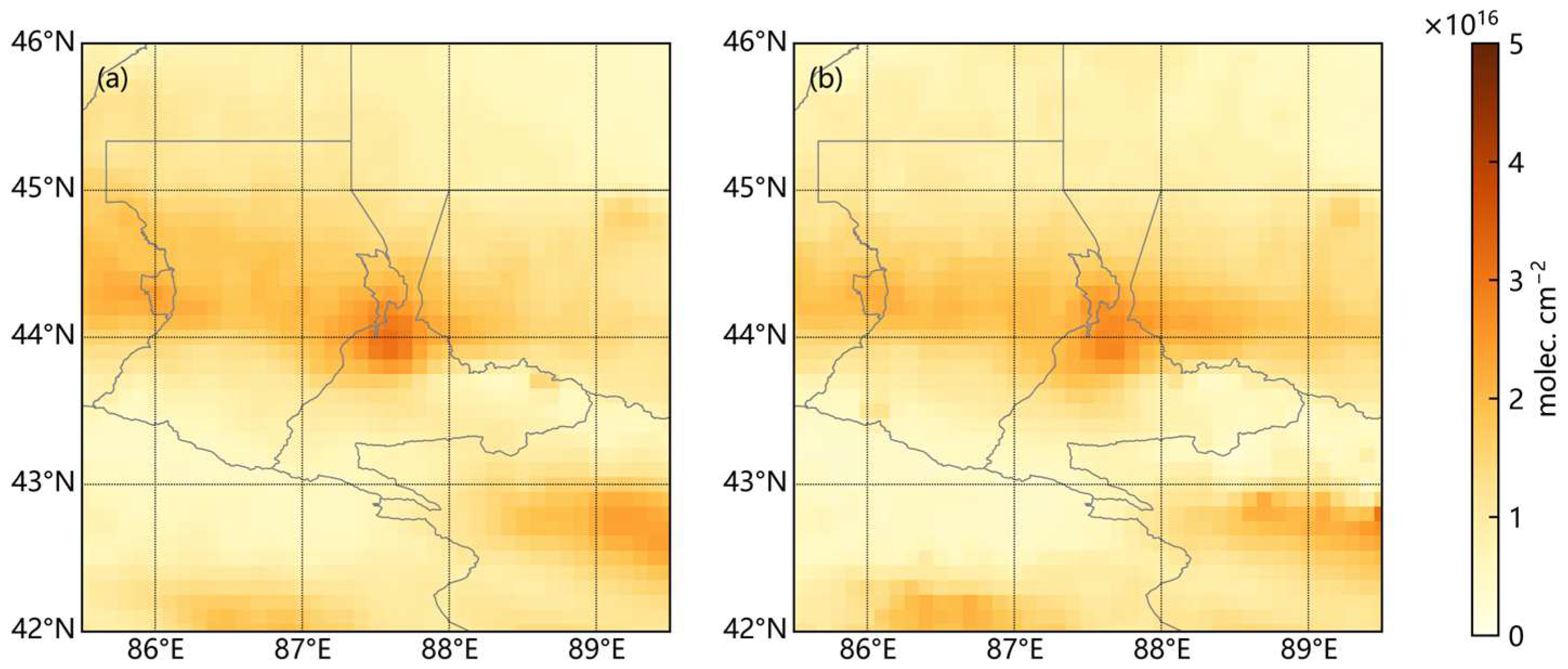
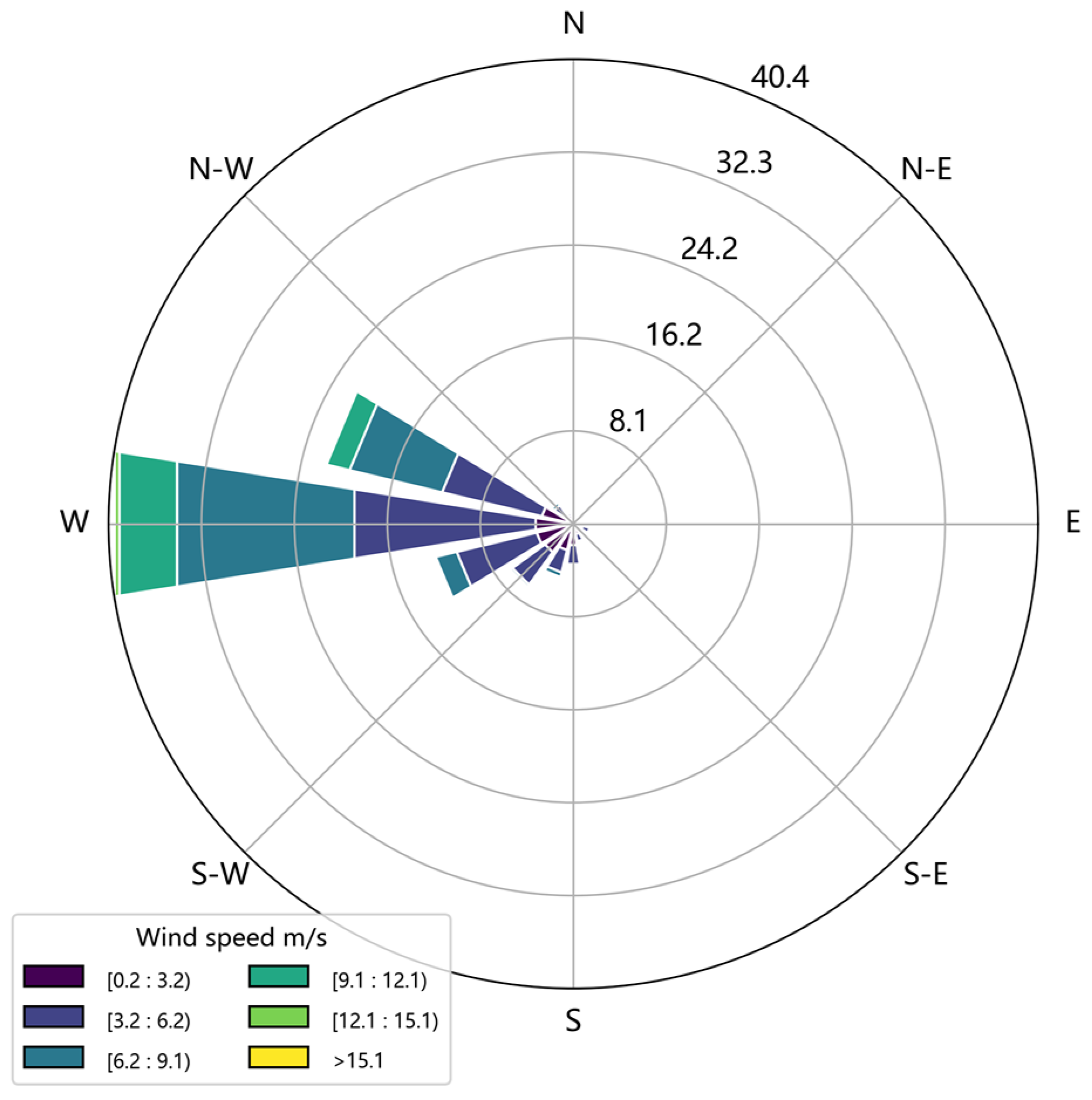
2.5. Selection of Study Area

Urumchi is the capital city of the Xinjiang Uygur Autonomous Region in the northwest of China. It is the largest city in Xinjiang region, and one of the most remote cities away from seas in the world [47]. It had a population of 4 million in 2022. At the end of 2022, there were 700 thousand grass-fed animals in Urumchi [48]. Urumchi is situated in a basin surrounded by the Tianshan Mountains to the north and south, and the city proper is located in the Dabancheng District, which lies in the eastern part of the basin. The city is at an elevation of approximately 800 m above sea level, and has a continental arid climate. The city is also situated along the ancient Silk Road trade route and serves as a hub for transportation and commerce in the region.
Golmud is a city located in the Haixi Mongol and Tibetan Autonomous Prefecture, in the province of Qinghai, China [49]. Golmud had a population of 0.14 million in 2022. At the end of 2022, there were 340 thousand grass-fed animals in Golmud [50]. It is situated in the northeastern part of the Qinghai-Tibet Plateau, at an elevation of 2809 m above sea level. The city is located near the Qilian Mountains to the north and the Kunlun Mountains to the south, surrounded by vast expanses of desert and grassland. The city has a dry and arid climate, with long and cold winter and a short and warm summer. It is an important transportation hub, connecting the western and eastern part of China, and also well known for its rich mineral resources, including salt, potassium, magnesium, and boron.
The city of Urumchi and Golmud are chosen for study for the following reasons: Firstly, NH3 total columns in Urumchi and Golmud are higher than those in the surrounding areas. Secondly, there are no large NH3 sources within 100 km radius of the two cities, so the interference from other sources is minimized. Figure 1 displays the locations of the two cities and the distributions of NH3 total column over China based on the dataset from the study of Van Damme et al. [13]. This dataset is taken from ANNI-NH3-v2.1R-I data, which are the oversampled data of IASI NH3 total columns for 9 years (2008–2016). The blue circles are the locations of Urumchi and Golmud.

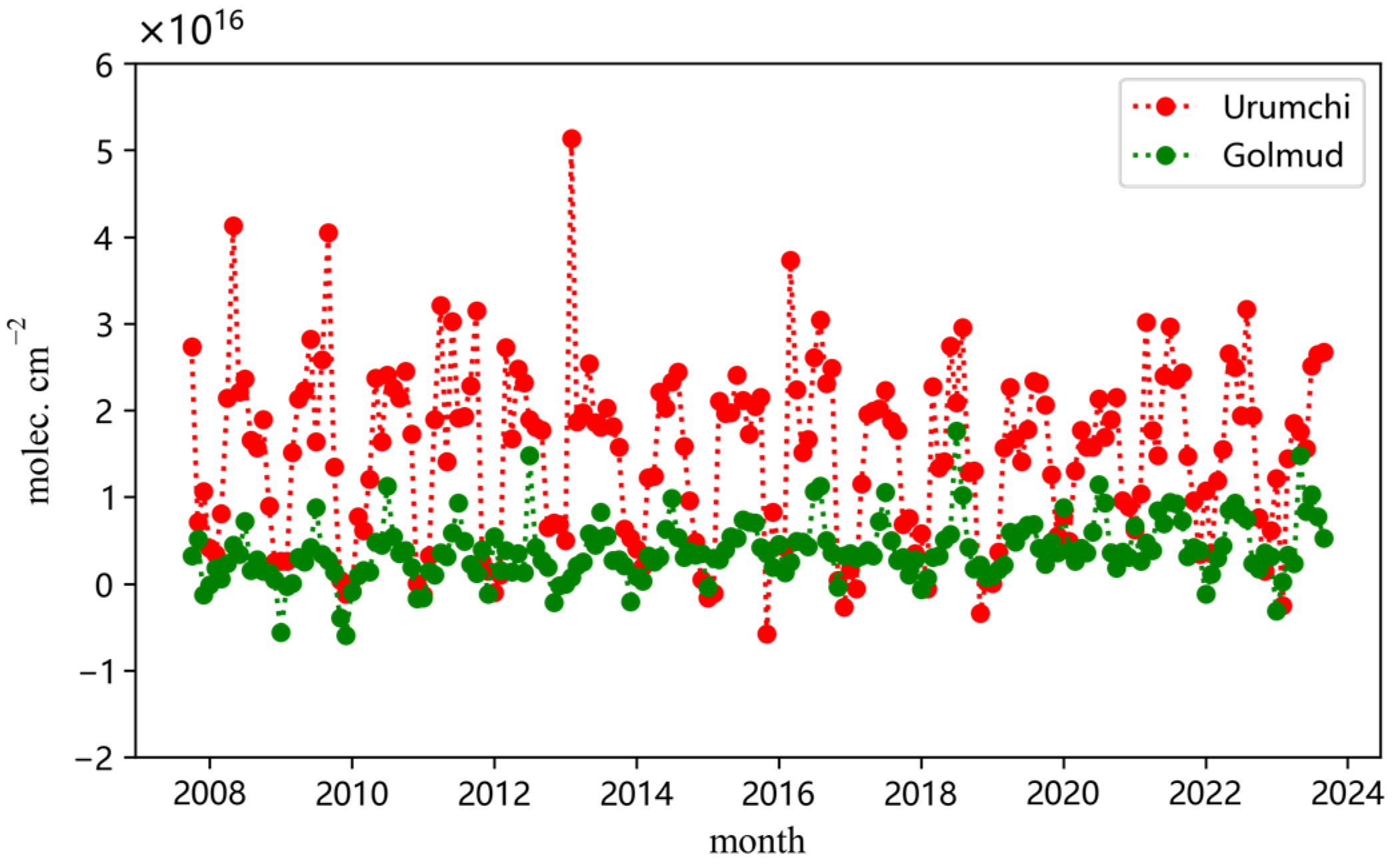
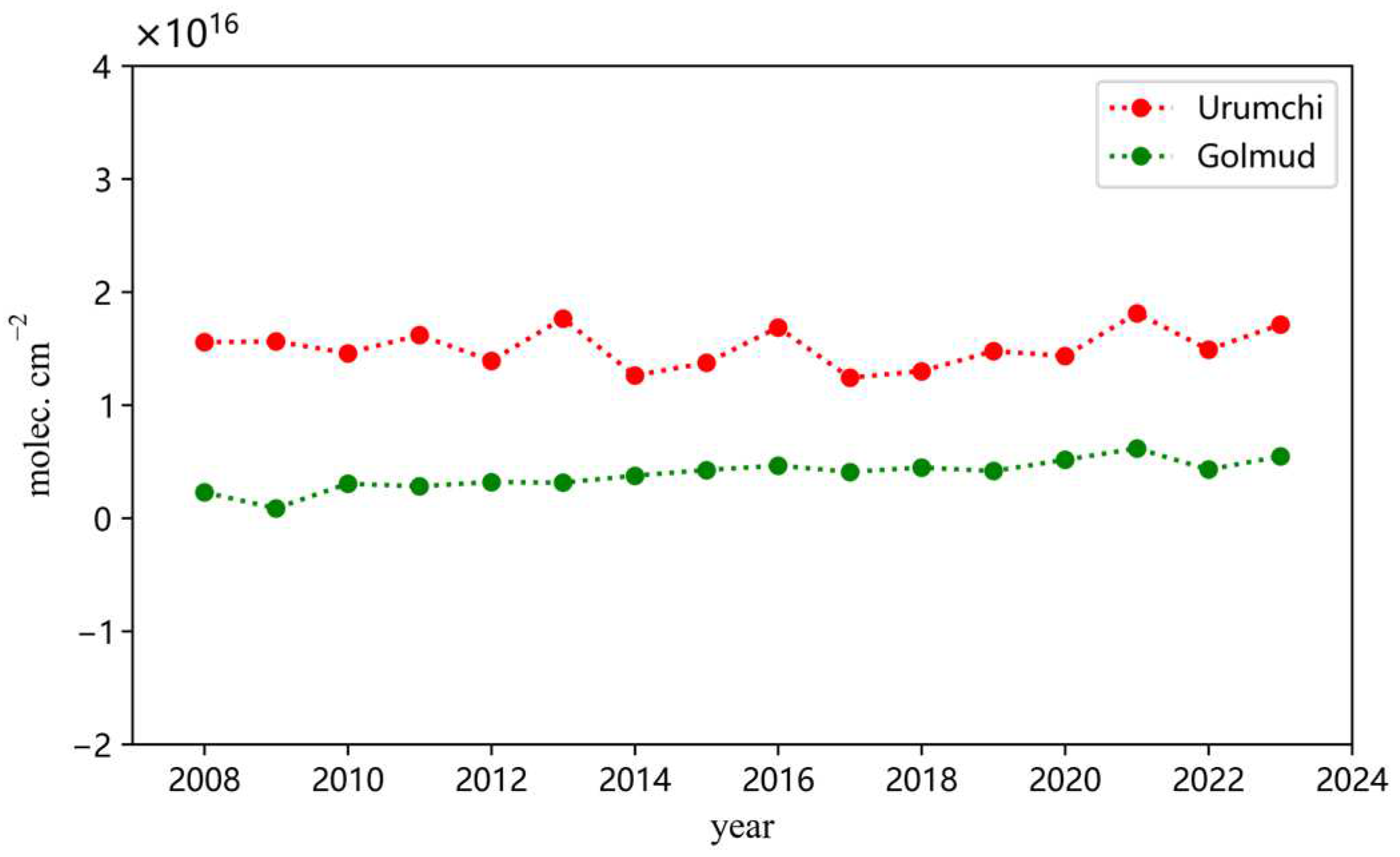
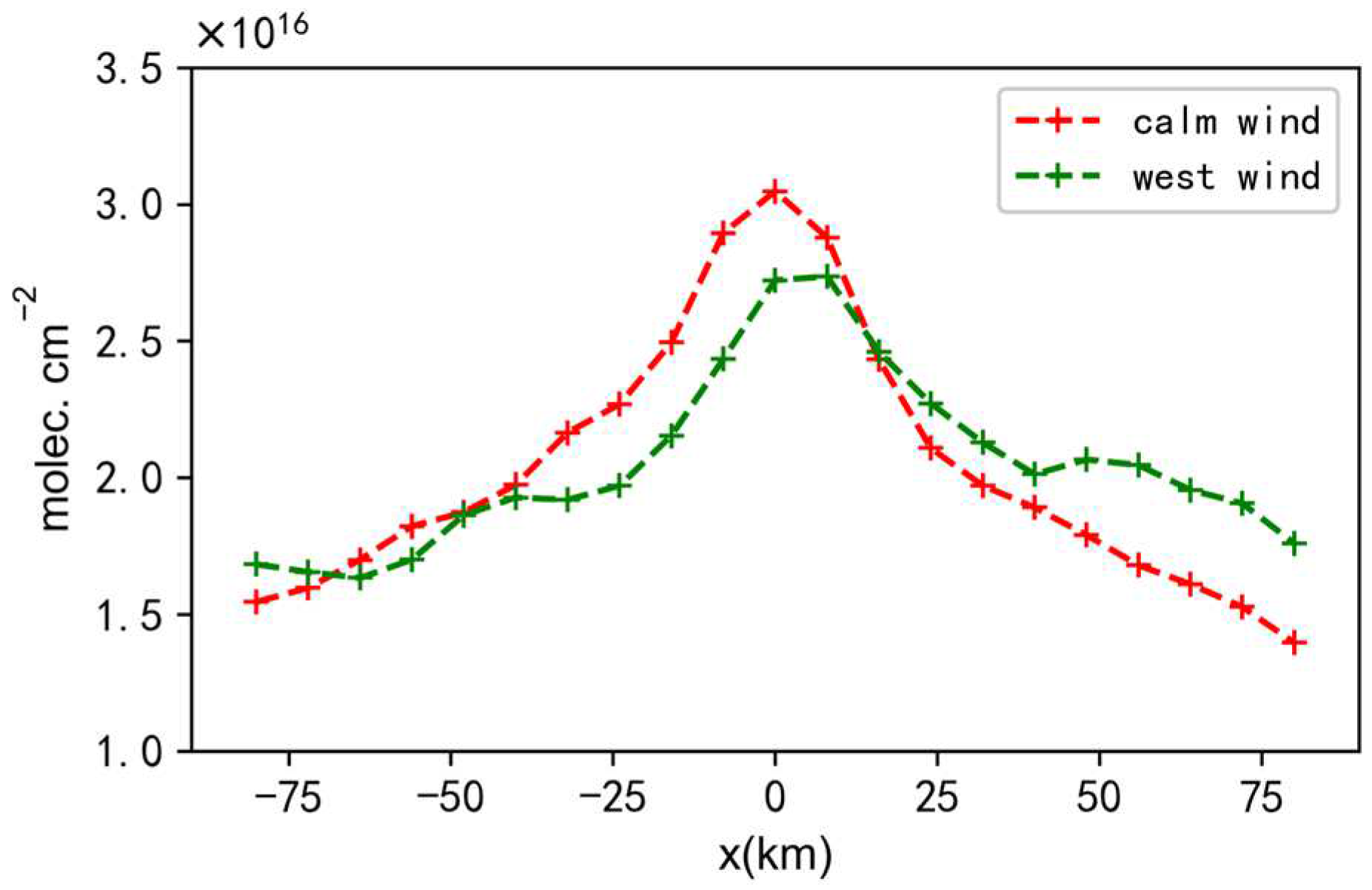
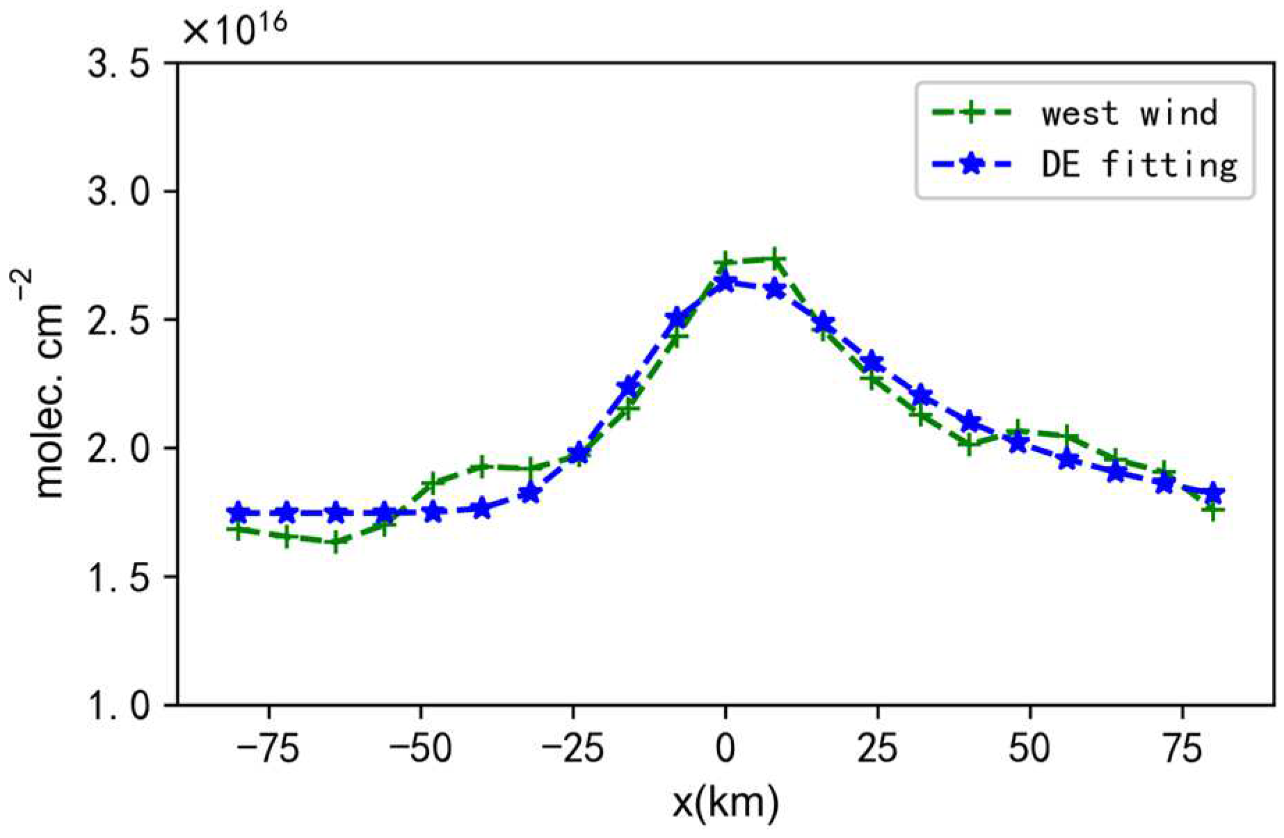
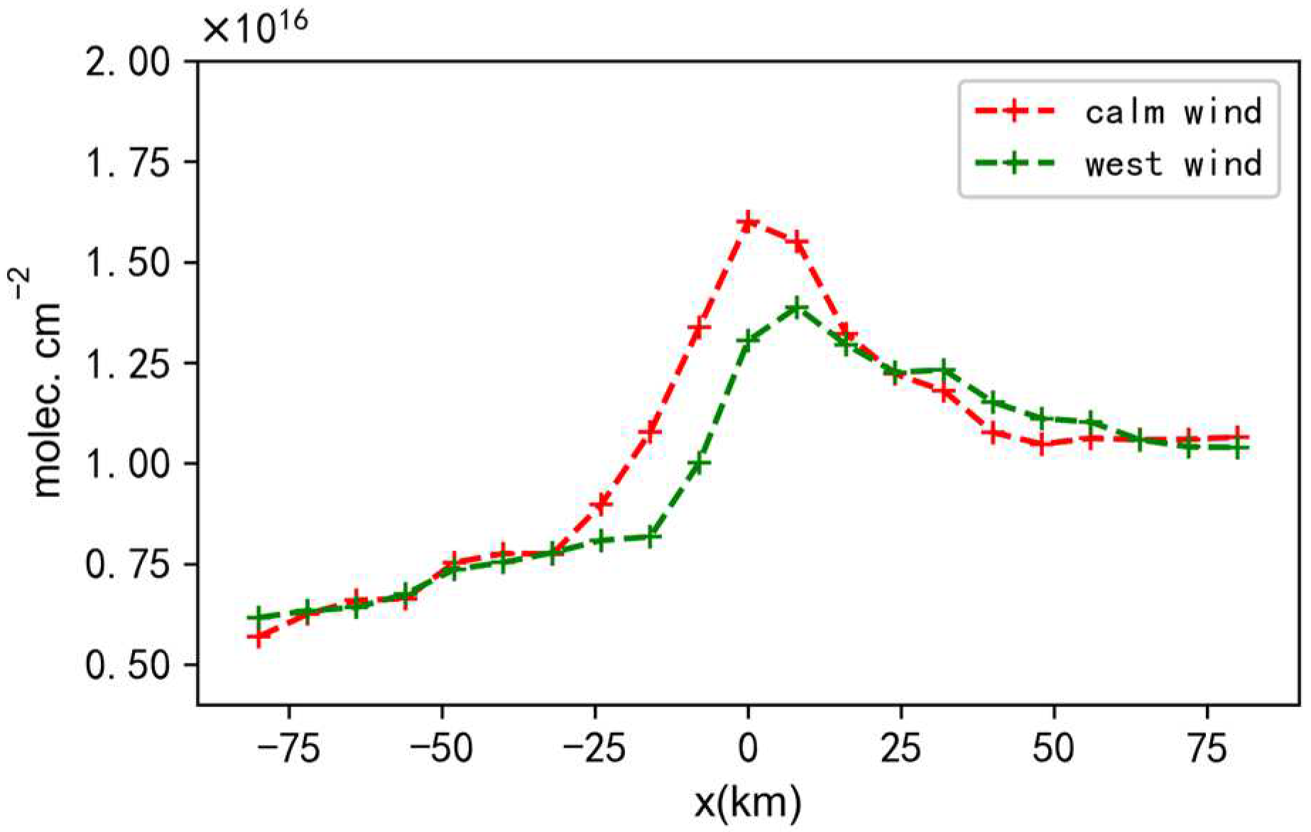
3. Results and Discussion

The monthly averages of NH3 total column in Urumchi and Golmud during from 2008 to 2023 were calculated based on IASI data, as shown in Figure 2. It can be seen that most NH3 total columns in Urumchi were higher than those in Golmud. So the annual averages of NH3 total columns in Urumchi are higher than the corresponding values in Golmud in Figure 3. Also, the annual averages of NH3 total columns in Urumchi show high levels in 2013, 2016, and 2021, with the value of 1.8 × 10¹⁶, 1.7 × 10¹⁶, and 1.8 × 10¹⁶ molec. cm−2, respectively. However, the variation of annual average of NH3 columns in Golmud shows a different pattern, with a slowly increasing trend and no peaks in different years.
Monthly averages of NH3 total columns throughout the observation period from 2008 to 2023 in Urumchi and Golmud were also calculated, as shown in Figure 4. NH3 total columns show obvious seasonal variation in Urumchi, with high concentrations from March to October and low concentrations in winter, such as in January, February, November, and December. Monthly averages of NH3 total columns are about 2.0 × 10¹⁶ molec. cm−2 from March to October, and about 4.7 × 10¹⁵ molec. cm−2 in winter in Urumchi. NH3 total columns also show clear seasonal variation in Golmud, with high concentrations in summer and low concentrations in winter. The monthly average of NH3 total columns reaches its maximum in July in Golmud, with a value of 1.0 × 10¹⁶ molec. cm−2.
Since ammonia is mainly concentrated near the surface, each IASI observation is linked to wind data from the surface to the height of 50 m taken from MERRA-2. We applied the DE method to determine the NH3 emissions and lifetime over Golmud and Urumchi city. Figure 5 plots the wind roses from MERRA-2 wind field data in Urumchi during “ozone season” (May–September) from 2008 to 2023. The main wind direction is west in Urumchi during the study period, so the variation of NH3 distributions under west wind and calm conditions is used to estimate emissions.
The NH3 emissions were estimated from the variation of NH3 distributions under windy and calm conditions. Figure 6 shows the distributions of the mean NH3 columns around Urumchi under calm and west wind conditions during “ozone season” (May–September) from 2008 to 2023. The outflow plume of NH3 in Urumchi clearly displays the distribution patterns of NH3 under different wind directions.
Figure 7 shows NH3 line densities under calm wind (red) and west wind (green) around Urumchi, and abscissa is the distance x to the center of Urumchi city. The maximum of the line density (red) appears in the center of the city under calm winds, and 8 km east of the city center under west wind conditions (green). The shift of the maximum of the two line densities under the two conditions reflects the spread range of the NH3 emission plume.
The fitted parameters by the DE algorithm are emissions E, background B, the e-folding distance x0, the fitted sources located in a polluted background relative to the Urumchi center X, and the standard deviation σ of the Gaussian function to describe the interference of different factors on the ideal distribution e(x). Figure 8 displays the fitted line density using the model function M(x) by the DE algorithm for the Urumchi area. The green line is the observed line density of ammonia under main wind direction, and the blue line is the fitted line density of ammonia.
NH3 emissions can be determined from the NH3 columns downwind decay. The lifetime (τ = x0/w) of NH3 is derived from the mean wind w and e-folding distance x0. For Urumchi, the NH3 emission estimated is 5.84 × 10⁻¹¹ kg·m−2s−1 and the lifetime of NH3 is computed to be 4.31 h during “ozone season” (May–September) from 2008 to 2023.
Figure 9 plots the wind roses from MERRA-2 wind field data in Golmud during “ozone season” (May–September) from 2008 to 2023. The main wind direction is also west in Golmud during the study period, so the variation of NH3 distributions under west wind and calm conditions is used to estimate emissions from Golmud area.
Figure 10 displays the mean NH3 columns around Golmud under calm and west wind conditions during “ozone season” (May–September) from 2008 to 2023. The outflow plume of NH3 in Golmud clearly displays the different distributions of NH3 columns under different wind directions. The different distributions of NH3 columns reflect the different plume dispersion regions under the two wind conditions.
Figure 11 shows NH3 line densities under west wind and calm wind around Golmud (Figure 11). The maximum of line density (red) appears in the center of the city under calm winds, and 7 km east of the city center under west wind conditions (green). The downwind shift of the maximum of line density under west wind also reflects the spread range of the emission plume. Figure 12 displays the fitted line densities using the model function M(x) by the DE algorithm for Golmud area, which is used for estimation of NH3 emissions. The green line is the observed line density of ammonia under the main wind direction, and the blue line is the fitted line density of ammonia. The NH3 emission is 4.19 × 10⁻¹¹ kg·m−2s−1 and the lifetime of NH3 is computed to be 9.19 h during “ozone season” (May–September) from 2008 to 2023 in Golmud.
The NH3 emissions in Golmud is slightly lower than that in Urumchi, as the emission sources are different in the two different areas. Firstly, the intensity of agricultural activities in the two cities is different, as the farming area and animal numbers fed in Urumqi are larger than those in Golmud. Secondly, more inhabitants in Urumqi means more anthropogenic emissions, such as those from transport, biomass burning, waste burning, and industry. These factors lead to high emission intensity from Urumqi city. Furthermore, the different lifetime of NH3 estimated in the two areas reflects the totally different sources and sinks. A shorter atmospheric lifetime of NH3 in Urumqi is likely caused by a higher emission of acidifying compounds (mostly SO2 and NOx) in the atmosphere. Moreover, more precipitation on average in Urumqi means more wet deposition in this area. These factors may explain the difference in ammonia lifetime in the two cities. The accuracy of emissions and lifetimes estimated by this work are highly depended on the accuracy of MERRA-2 wind directions and the satellite observations. There are potential sources of uncertainty contributing to the estimation results. First is the uncertainty of total columns of ammonia from satellite data due to retrieval methods and hardware. Second is fit errors due to calculation of the line density. Third is from wind fields, as wind information is important during fit for determination of the fitted parameters.
Further, in order to validate our results, we compared our results with those in other studies. Table 1 lists the comparison of our results with the emission values reported in some emission inventories. Anthropogenic sources in the REAS emission inventory include power plant, domestic, fertilizer, manure management, industry, road transport, other transport, and miscellaneous sources. Anthropogenic sources in the EDGAR emission inventory include agriculture, power, industry, residential, transportation, and other sources. Anthropogenic sources in the MEIC-PKU-NH3 emission inventory include power plant, industry, residential, transportation, agriculture, and wildfire. In this study, anthropogenic sources in the two cities include agriculture, power, industry, residential, transportation, and other sources, while the natural sources may include soils and plants. Table 1 shows that the NH3 emission of Urumchi derived in this study agrees well with the values from the EDGAR and MEIC-PKU emission inventory, but is less than the value from the REAS emission inventory. While the NH3 emission of Golmud derived in this study is lower than the value from the REAS emission inventory, and higher than the values from the EDGAR and MEIC-PKU emission inventory, the emission estimated in our study is close to the values reported in these emission inventories. The comparison results prove the reliability of the emission estimation method used in this study.
Moreover, Table 2 displays the comparison of the estimated lifetime of NH3 with the values reported in publications. The lifetime of NH3 reported in other studies is in the range between 2.5 and 36 h, and the values estimated in Urumchi and Golmud of 4.31 and 9.19 h fall into this range, which also proves the reliability of the estimation method used in this study.

4. Conclusions

Ammonia is a short-lived trace gas and satellite data are sparse, which makes it difficult to estimate NH3 emissions from urban sources. In this study, we used the DE optimization algorithm to estimate the ammonia emissions and lifetime over two inland cities in China, based on the IASI satellite data and wind fields for the period (May–September) from 2008 to 2023.
The NH3 emission rate estimated is 5.84 × 10⁻¹¹ and 4.19 × 10⁻¹¹ kg·m−2s−1 in the Urumchi and Golmud areas, respectively. The lifetime of NH3 is 4.31 h and 9.19 h, respectively, in these two areas. The different emissions and different lifetime of NH3 estimated in the two cities reflects the distinct sources and sinks in the two areas. Firstly, the intensity of agricultural activities related to manure management and fertilizer application in the two cities is different. Secondly, different numbers of inhabitants means different anthropogenic emissions from transport, biomass burning, waste burning, and industry. Thirdly, different levels of acidifying compounds (mostly SO2 and NOx) in the atmosphere mean different conversion rate to particulate ammonium salts via reaction with acids. Lastly, different weather conditions lead to different dry deposition and wet removal. All these factors result in the different emissions and lifetime of ammonia in the two cities. We compared the NH3 emissions and lifetime estimated in this study with the values in other studies, and the results show the reliability of the method used. This work is one of few quantitative studies of NH3 emissions and lifetime from cities in China using satellite observations. Our study provides a valuable method for quantification of urban ammonia emissions, helping to control ammonia emissions from cities and evaluate the effectiveness of control measures, especially for cities with high concentrations of ammonia.
In summary, satellite observations offer a valuable insight into ammonia emissions and atmospheric processes. While satellite observations can resolve isolated urban sources and estimate the emissions from cities, it is difficult for satellite data to distinguish anthropogenic emissions from natural emissions. This problem can be resolved by conventional emission inventories. Combining satellite observations with ground-based measurements and refining modeling based on emission inventories can contribute to a more comprehensive understanding of ammonia dynamics in the atmosphere.

Author Contributions

Conceptualization, Y.X.; project administration, W.W.; supervision, X.H.; validation, Z.C.; writing—original draft, K.C., Y.C. and Z.Q.; visualization, J.C., J.T., L.L. and Y.Y. All authors have read and agreed to the published version of the manuscript.

Funding

This research was funded by University Natural Sciences Research Project of Anhui Province (Project Number: 2022AH051794, 2022AH051793) and Anhui Provincial New Era Education Quality Project (Project Number: 2022xxsfkc049, 2022tsxwd048).

Institutional Review Board Statement

Not applicable.

Informed Consent Statement

Not applicable.

Data Availability Statement

The IASI ammonia (NH3) total columns dataset (Metop-A https://doi.org/10.25326/10 (accessed on 20 February 2024), Metop-B https://doi.org/10.25326/11 (accessed on 20 February 2024)). The reanalyzed daily IASI ammonia (NH3) total column dataset (Metop-A https://doi.org/10.25326/12 (accessed on 20 February 2024), Metop-B https://doi.org/10.25326/13 (accessed on 20 February 2024)). The MERRA-2 data used in this study have been provided by the Global Modeling and Assimilation Office (GMAO) at NASA Goddard Space Flight Center through the online data portal in the Goddard Earth Sciences Data and Information Services Center, 10.5067/3Z173KIE2TPD. It can be downloaded from website (https://disc.gsfc.nasa.gov/datasets/M2I1NXASM_5.12.4/summary (accessed on 20 February 2024)).

Conflicts of Interest

The authors declare no conflicts of interest. The funders had no role in the design of the study; in the collection, analyses, or interpretation of data; in the writing of the manuscript; or in the decision to publish the results.

References

  1. Diana, M.P.; Roekmijati, W.S.; Suyud, W.U. Why it is often underestimated: Historical study of ammonia gas exposure impacts towards human health. In Proceedings of the 3rd International Conference on Energy, Environmental and Information System (ICENIS 2018), Semarang, Indonesia, 14–15 August 2018; p. 06003. [Google Scholar]
  2. Wyer, K.E.; Kelleghan, D.B.; Blanes-Vidal, V.; Schauberger, G.; Curran, T.P. Ammonia emissions from agriculture and their contribution to fine particulate matter: A review of implications for human health. J. Environ. Manag. 2022, 323, 116285. [Google Scholar] [CrossRef]
  3. Spector, O.; Jacobson, E. Advanced ammonia (NH3) monitoring system for industrial applications. In Proceedings of the Photonics East ‘99, Boston, MA, USA, 21 December 1999. [Google Scholar]
  4. Peng, R.D.; Bell, M.L.; Geyh, A.S.; McDermott, A.; Zeger, S.L.; Samet, J.M.; Dominici, F. Emergency admissions for cardiovascular and respiratory diseases and the chemical composition of fine particle air pollution. Environ. Health Perspect. 2009, 117, 957–963. [Google Scholar] [CrossRef] [PubMed]
  5. Diacono, M.; Montemurro, F. Long-Term Effects of Organic Amendments on Soil Fertility. Sustain. Agric. 2011, 2, 761–786. [Google Scholar]
  6. Shin, M.; Kang, Y.; Park, S.; Im, J.; Yoo, C.; Quackenbush, L.J. Estimating ground-level particulate matter concentrations using satellite-based data: A review. GISci. Remote Sens. 2020, 57, 174–189. [Google Scholar] [CrossRef]
  7. Jiang, L.; He, S.; Zhou, H.; Kong, H.; Wang, J.; Cui, Y.; Wang, L. Coordination between sulfur dioxide pollution control and rapid economic growth in China: Evidence from satellite observations and spatial econometric models. Struct. Chang. Econ. Dyn. 2021, 57, 279–291. [Google Scholar] [CrossRef]
  8. Vîrghileanu, M.; Săvulescu, I.; Mihai, B.-A.; Nistor, C.; Dobre, R. Nitrogen Dioxide (NO2) Pollution monitoring with Sentinel-5P satellite imagery over Europe during the coronavirus pandemic outbreak. Remote Sens. 2020, 12, 3575. [Google Scholar] [CrossRef]
  9. Wang, W.; van der A, R.; Ding, J.; van Weele, M.; Cheng, T. Spatial and temporal changes of the ozone sensitivity in China based on satellite and ground-based observations. Atmos. Chem. Phys. 2021, 21, 7253–7269. [Google Scholar] [CrossRef]
  10. Liu, F.; Duncan, B.N.; Krotkov, N.A.; Lamsal, L.N.; Beirle, S.; Griffin, D.; McLinden, C.A.; Goldberg, D.L.; Lu, Z. A methodology to constrain carbon dioxide emissions from coal-fired power plants using satellite observations of co-emitted nitrogen dioxide. Atmos. Chem. Phys. 2020, 20, 99–116. [Google Scholar] [CrossRef]
  11. Zhang, X.; Liu, J.; Han, H.; Zhang, Y.; Jiang, Z.; Wang, H.; Meng, L.; Li, Y.C.; Liu, Y. Satellite-observed variations and trends in carbon monoxide over Asia and their sensitivities to biomass burning. Remote Sens. 2020, 12, 830. [Google Scholar] [CrossRef]
  12. De Gouw, J.A.; Veefkind, J.P.; Roosenbrand, E.; Dix, B.; Lin, J.C.; Landgraf, J.; Levelt, P.F. Daily satellite observations of methane from oil and gas production regions in the United States. Sci. Rep. 2020, 10, 1379. [Google Scholar] [CrossRef]
  13. Van Damme, M.; Clarisse, L.; Whitburn, S.; Hadji-Lazaro, J.; Hurtmans, D.; Clerbaux, C.; Coheur, P.-F. Industrial and agricultural ammonia point sources exposed. Nature 2018, 564, 99–103. [Google Scholar] [CrossRef]
  14. Irakulis-Loitxate, I.; Guanter, L.; Liu, Y.-N.; Varon, D.J.; Maasakkers, J.D.; Zhang, Y.; Chulakadabba, A.; Wofsy, S.C.; Thorpe, A.K.; Duren, R.M. Satellite-based survey of extreme methane emissions in the Permian basin. Sci. Adv. 2021, 7, eabf4507. [Google Scholar] [CrossRef]
  15. Zhang, X.; Wang, F.; Wang, W.; Huang, F.; Chen, B.; Gao, L.; Wang, S.; Yan, H.; Ye, H.; Si, F. The development and application of satellite remote sensing for atmospheric compositions in China. Atmos. Res. 2020, 245, 105056. [Google Scholar] [CrossRef]
  16. Yi, L.; Jing, W.; Ke, C.; Zhaonan, C.; Dongxu, Y.; Lin, W. Satellite remote sensing of greenhouse gases: Progress and trends. Natl. Remote Sens. Bull. 2021, 25, 53–64. [Google Scholar] [CrossRef]
  17. Elguindi, N.; Granier, C.; Stavrakou, T.; Darras, S.; Bauwens, M.; Cao, H.; Chen, C.; Denier van der Gon, H.; Dubovik, O.; Fu, T. Intercomparison of magnitudes and trends in anthropogenic surface emissions from bottom-up inventories, top-down estimates, and emission scenarios. Earth’s Future 2020, 8, e2020EF001520. [Google Scholar] [CrossRef]
  18. Laughner, J.L.; Cohen, R.C. Direct observation of changing NOx lifetime in North American cities. Science 2019, 366, 723–727. [Google Scholar] [CrossRef]
  19. Marais, E.A.; Pandey, A.K.; Van Damme, M.; Clarisse, L.; Coheur, P.F.; Shephard, M.W.; Cady-Pereira, K.E.; Misselbrook, T.; Zhu, L.; Luo, G.; et al. UK ammonia emissions estimated with satellite observations and GEOS-Chem. J. Geophys. Res. Atmos. 2021, 126, e2021JD035237. [Google Scholar] [CrossRef]
  20. Fu, Y.; Sun, W.; Fan, D.; Zhang, Z.; Hao, Y. An assessment of China’s industrial emission characteristics using satellite observations of XCO2, SO2, and NO2. Atmos. Pollut. Res. 2022, 13, 101486. [Google Scholar] [CrossRef]
  21. Beirle, S.; Boersma, K.F.; Platt, U.; Lawrence, M.G.; Wagner, T. Megacity emissions and lifetimes of nitrogen oxides probed from space. Science 2011, 333, 1737–1739. [Google Scholar] [CrossRef] [PubMed]
  22. Liu, F.; Beirle, S.; Zhang, Q.; Dörner, S.; He, K.; Wagner, T. NOx lifetimes and emissions of cities and power plants in polluted background estimated by satellite observations. Atmos. Chem. Phys. 2016, 16, 5283–5298. [Google Scholar] [CrossRef]
  23. Liu, F.; Beirle, S.; Zhang, Q.; van der A, R.J.; Zheng, B.; Tong, D.; He, K. NOx emission trends over Chinese cities estimated from OMI observations during 2005 to 2015. Atmos. Chem. Phys. 2017, 17, 9261–9275. [Google Scholar] [CrossRef] [PubMed]
  24. Liu, F.; Tao, Z.; Beirle, S.; Joiner, J.; Yoshida, Y.; Smith, S.J.; Knowland, K.E.; Wagner, T. A new method for inferring city emissions and lifetimes of nitrogen oxides from high-resolution nitrogen dioxide observations: A model study. Atmos. Chem. Phys. 2022, 22, 1333–1349. [Google Scholar] [CrossRef]
  25. Zhang, X.; Lu, X.; Chuai, X.; Wang, Z.; Wu, X. Trade-driven relocation of ground-level SO2 concentrations across Chinese provinces based on satellite observations. Environ. Sci. Pollut. Res. 2023, 30, 14619–14629. [Google Scholar] [CrossRef] [PubMed]
  26. Kourtidis, K.; Georgoulias, A.K.; Mijling, B.; van der A, R.; Zhang, Q.; Ding, J. A new method for deriving trace gas emission inventories from satellite observations: The case of SO2 over China. Sci. Total Environ. 2018, 612, 923–930. [Google Scholar] [CrossRef] [PubMed]
  27. Wang, S.; Xing, J.; Chatani, S.; Hao, J.; Klimont, Z.; Cofala, J.; Amann, M. Verification of anthropogenic emissions of China by satellite and ground observations. Atmos. Environ. 2011, 45, 6347–6358. [Google Scholar] [CrossRef]
  28. Zhang, L.; Chen, Y.; Zhao, Y.; Henze, D.K.; Zhu, L.; Song, Y.; Paulot, F.; Liu, X.; Pan, Y.; Lin, Y.; et al. Agricultural ammonia emissions in China: Reconciling bottom-up and top-down estimates. Atmos. Chem. Phys. 2018, 18, 339–355. [Google Scholar] [CrossRef]
  29. Van Damme, M.; Clarisse, L.; Franco, B.; Sutton, M.A.; Erisman, J.W.; Wichink Kruit, R.; van Zanten, M.; Whitburn, S.; Hadji-Lazaro, J.; Hurtmans, D.; et al. Global, regional and national trends of atmospheric ammonia derived from a decadal (2008–2018) satellite record. Environ. Res. Lett. 2021, 16, 055017. [Google Scholar] [CrossRef]
  30. Clarisse, L.; Van Damme, M.; Clerbaux, C.; Coheur, P.F. Tracking down global NH3 point sources with wind-adjusted superresolution. Atmos. Meas. Tech. 2019, 12, 5457–5473. [Google Scholar] [CrossRef]
  31. Clarisse, L.; Van Damme, M.; Gardner, W.; Coheur, P.F.; Clerbaux, C.; Whitburn, S.; Hadji-Lazaro, J.; Hurtmans, D. Atmospheric ammonia (NH3) emanations from Lake Natron’s saline mudflats. Sci. Rep. 2019, 9, 4441. [Google Scholar] [CrossRef]
  32. Dammers, E.; McLinden, C.A.; Griffin, D.; Shephard, M.W.; Van Der Graaf, S.; Lutsch, E.; Schaap, M.; Gainairu-Matz, Y.; Fioletov, V.; Van Damme, M.; et al. NH3 emissions from large point sources derived from CrIS and IASI satellite observations. Atmos. Chem. Phys. 2019, 19, 12261–12293. [Google Scholar] [CrossRef]
  33. Li, B.; Chen, L.; Shen, W.; Jin, J.; Wang, T.; Wang, P.; Yang, Y.; Liao, H. Improved gridded ammonia emission inventory in China. Atmos. Chem. Phys. 2021, 21, 15883–15900. [Google Scholar] [CrossRef]
  34. Hauglustaine, D.A.; Balkanski, Y.; Schulz, M. A global model simulation of present and future nitrate aerosols and their direct radiative forcing of climate. Atmos. Chem. Phys. 2014, 14, 11031–11063. [Google Scholar] [CrossRef]
  35. Shephard, M.W.; Dammers, E.; Cady-Pereira, K.E.; Kharol, S.K.; Thompson, J.; Gainariu-Matz, Y.; Zhang, J.; McLinden, C.A.; Kovachik, A.; Moran, M.; et al. Ammonia measurements from space with the Cross-track Infrared Sounder: Characteristics and applications. Atmos. Chem. Phys. 2020, 20, 2277–2302. [Google Scholar] [CrossRef]
  36. Abeed, R.; Viatte, C.; Porter, W.C.; Evangeliou, N.; Clerbaux, C.; Clarisse, L.; Van Damme, M.; Coheur, P.F.; Safieddine, S. A roadmap to estimating agricultural ammonia volatilization over Europe using satellite observations and simulation data. Atmos. Chem. Phys. 2023, 23, 12505–12523. [Google Scholar] [CrossRef]
  37. Evangeliou, N.; Balkanski, Y.; Eckhardt, S.; Cozic, A.; Van Damme, M.; Coheur, P.F.; Clarisse, L.; Shephard, M.W.; Cady-Pereira, K.E.; Hauglustaine, D. 10-year satellite-constrained fluxes of ammonia improve performance of chemistry transport models. Atmos. Chem. Phys. 2021, 21, 4431–4451. [Google Scholar] [CrossRef]
  38. Whitburn, S.; Van Damme, M.; Clarisse, L.; Turquety, S.; Clerbaux, C.; Coheur, P.-F. Doubling of annual ammonia emissions from the peat fires in Indonesia during the 2015 El Niño. Geophys. Res. Lett. 2016, 43, 11007–11014. [Google Scholar] [CrossRef]
  39. Franco, B.; Clarisse, L.; Stavrakou, T.; Müller, J.-F.; Van Damme, M.; Whitburn, S.; Hadji-Lazaro, J.; Hurtmans, D.; Taraborrelli, D.; Clerbaux, C.; et al. A General Framework for Global Retrievals of Trace Gases From IASI: Application to Methanol, Formic Acid, and PAN. J. Geophys. Res. Atmos. 2018, 123, 13963–13984. [Google Scholar] [CrossRef]
  40. Clarisse, L.; Franco, B.; Van Damme, M.; Di Gioacchino, T.; Hadji-Lazaro, J.; Whitburn, S.; Noppen, L.; Hurtmans, D.; Clerbaux, C.; Coheur, P. The IASI NH3 version 4 product: Averaging kernels and improved consistency. Atmos. Meas. Tech. 2023, 2023, 5009–5028. [Google Scholar] [CrossRef]
  41. Van Damme, M.; Whitburn, S.; Clarisse, L.; Clerbaux, C.; Hurtmans, D.; Coheur, P.F. Version 2 of the IASI NH3 neural network retrieval algorithm: Near-real-time and reanalysed datasets. Atmos. Meas. Tech. 2017, 10, 4905–4914. [Google Scholar] [CrossRef]
  42. Whitburn, S.; Van Damme, M.; Clarisse, L.; Bauduin, S.; Heald, C.L.; Hadji-Lazaro, J.; Hurtmans, D.; Zondlo, M.A.; Clerbaux, C.; Coheur, P.F. A flexible and robust neural network IASI-NH3 retrieval algorithm. J. Geophys. Res. Atmos. 2016, 121, 6581–6599. [Google Scholar] [CrossRef]
  43. Guthrie, S.; Harshfield, A.; Ioppolo, B.; Dunkerley, F.; Manville, C.; Tabaqchali, H.; Giles, S. Impact of Ammonia Emissions from Agriculture on Biodiversity: An Evidence Synthesis; The Royal Society: London, UK, 2018. [Google Scholar]
  44. Liu, X.; Tai, A.P.K.; Fung, K.M. Responses of surface ozone to future agricultural ammonia emissions and subsequent nitrogen deposition through terrestrial ecosystem changes. Atmos. Chem. Phys. 2021, 21, 17743–17758. [Google Scholar] [CrossRef]
  45. Gelaro, R.; McCarty, W.; Suárez, M.J.; Todling, R.; Molod, A.; Takacs, L.; Randles, C.A.; Darmenov, A.; Bosilovich, M.G.; Reichle, R.; et al. The Modern-Era Retrospective Analysis for Research and Applications, Version 2 (MERRA-2). J. Clim. 2017, 30, 5419–5454. [Google Scholar] [CrossRef]
  46. Storn, R.; Price, K. Differential evolution–a simple and efficient heuristic for global optimization over continuous spaces. J. Glob. Optim. 1997, 11, 341–359. [Google Scholar] [CrossRef]
  47. Dong, W.; Zhang, X. Urumqi. Cities 2011, 28, 115–125. [Google Scholar] [CrossRef]
  48. National Bureau of Statistics of China. Statistical Communique on National Economic and Social Development of Urumchi City in 2022. Available online: http://www.urumqi.gov.cn/fjbm/tjj/tjgb/530376.htm (accessed on 20 February 2024).
  49. Wikipedia Contributors. Golmud. Available online: https://en.wikipedia.org/w/index.php?title=Golmud&oldid=1177302641 (accessed on 20 February 2024).
  50. Statistical Communique on National Economic and Social Development of Golmud City in 2022. 2023. Available online: https://www.geermu.gov.cn/details?id=bb5cf28b86ab19500186e9af21bf0195 (accessed on 20 February 2024).
  51. Kurokawa, J.; Ohara, T. Long-term historical trends in air pollutant emissions in Asia: Regional Emission inventory in ASia (REAS) version 3. Atmos. Chem. Phys. 2020, 20, 12761–12793. [Google Scholar] [CrossRef]
  52. Monforti-Ferrario, F.; Crippa, M.; Guizzardi, D.; Muntean, M.; Schaaf, E.; Banja, M.; Pagani, F.; Solazzo, E. EDGAR v6. 1 Global Air Pollutant Emissions; European Commission, Joint Research Centre (JRC). Available online: http://data.europa.eu/89h/df521e05-6a3b-461c-965a-b703fb62313e (accessed on 20 February 2024).
  53. Meng, W.; Zhong, Q.; Yun, X.; Zhu, X.; Huang, T.; Shen, H.; Chen, Y.; Chen, H.; Zhou, F.; Liu, J. Improvement of a global high-resolution ammonia emission inventory for combustion and industrial sources with new data from the residential and transportation sectors. Environ. Sci. Technol. 2017, 51, 2821–2829. [Google Scholar] [CrossRef]
Figure 1. The locations of Urumchi and Golmud and IASI NH3 mean total column distribution of China during from 2008 to 2016. The locations of Urumchi and Golmud are marked by blue circles.
Atmosphere 15 00251 g001
Figure 2. Variation of monthly average of NH3 total columns in Urumchi and Golmud.
Atmosphere 15 00251 g002
Figure 3. Variation of annual average of NH3 total columns in Urumchi and Golmud.
Atmosphere 15 00251 g003
Figure 4. Monthly average of NH3 total columns throughout the observation period from 2008 to 2023 in Urumchi and Golmud.
Atmosphere 15 00251 g004
Figure 5. Wind roses from MERRA-2 wind field data in Urumchi during the study period.
Atmosphere 15 00251 g005
Figure 6. Mean NH3 columns around Urumchi under (a) calm and (b) west wind conditions.
Atmosphere 15 00251 g006
Figure 7. NH3 line densities under calm wind (red) and west wind (green) around Urumchi as a function of the distance x to Urumchi center.
Atmosphere 15 00251 g007
Figure 8. The fitted line density using the model function M(x) by the DE algorithm for the Urumchi area.
Atmosphere 15 00251 g008
Figure 9. Wind roses of MERRA-2 model at Golmud during the research period.
Atmosphere 15 00251 g009
Figure 10. Mean NH3 columns around Golmud under (a) calm and (b) west wind conditions.
Atmosphere 15 00251 g010
Figure 11. NH3 line densities under calm wind (red) and east wind (green) around Golmud as a function of the distance x to Golmud center.
Atmosphere 15 00251 g011
Figure 12. The fitted line density using the model function M(x) by the DE algorithm for the Golmud area.
Atmosphere 15 00251 g012
Table 1. NH3 emissions estimated compared with emission inventories.
MethodSourceUrumchiGolmud
REASv3.2.1 [51]anthropogenic sources2.83 × 10−10 kg·m−2s−11.59 × 10⁻¹⁰ kg·m−2s−1
EDGAR V6.1 [52]anthropogenic sources5.43 × 10−11 kg·m−2s−14.48 × 10⁻¹² kg·m−2s−1
MEIC-PKU-NH3 [53]anthropogenic sources5.06 × 10−11 kg·m−2s−12.22 × 10⁻¹² kg·m−2s−1
This studyanthropogenic sources and natural sources5.84 × 10−11 kg·m−2s−14.19 × 10⁻¹¹ kg·m−2s−1
Table 2. NH3 lifetime estimated compared with those reported in publications.
ReferenceDataMethodLifetime
Van Damme et al., 2018 [13]IASIBox modelSmaller than 12 h
Dammers et al., 2019 [32]CrIS, IASIWind rotation and EMG method∼2.5 h
(Hauglustaine et al., 2014 [34]AeroCom emission data setLMDz-INCA global model∼15 h
Shephard et al., 2020 [35]CrIS2-D EMG method∼2.66 h
Abeed et al., 2023 [36]IASIGEOS-Chem model∼6 h
Evangeliou et al., 2021 [37]IASI, CrISInverse distance weighting∼11.6 h
Whitburn et al., 2016 [38]IASIBox modelbetween 12 and 36h
This studyIASILine density model4.31 h and 9.19 h
Disclaimer/Publisher’s Note: The statements, opinions and data contained in all publications are solely those of the individual author(s) and contributor(s) and not of MDPI and/or the editor(s). MDPI and/or the editor(s) disclaim responsibility for any injury to people or property resulting from any ideas, methods, instructions or products referred to in the content.

