Article

Connecting Global Modes of Variability to Climate in High Mountain Asia

1
Computational Sciences and Engineering Division, Oak Ridge National Laboratory, Oak Ridge, TN 37830, USA
2
Department of Environmental Science, Policy, and Management, University of California Berkeley, Berkeley, CA 94720, USA
3
Global Modeling & Assimilation Office, NASA Goddard Space Flight Center, Greenbelt, MD 20771, USA
4
Goddard Earth Sciences Technology and Research (GESTAR) II, University of Maryland, Baltimore County, Baltimore, MD 21250, USA
*
Author to whom correspondence should be addressed.
Atmosphere 2024, 15(2), 142; https://doi.org/10.3390/atmos15020142
Submission received: 9 November 2023 / Revised: 10 January 2024 / Accepted: 16 January 2024 / Published: 23 January 2024
(This article belongs to the Section Climatology)

Abstract

:
Oscillations in global modes of variability (MoVs) form global teleconnections that affect regional climate variability and modify the potential for severe and damaging weather conditions. Understanding the link between certain MoVs and regional climate can improve the ability to more accurately predict environmental conditions that impact human life and health. In this study, we explore the connection between different MoVs, including the Arctic oscillation (AO), Eurasian teleconnection, Indian Ocean dipole (IOD), North Atlantic oscillation (NAO), and El Niño southern oscillation (Nino34), with winter and summer climates in the High Mountain Asia (HMA) region, including geopotential height at 250 hPa (z250), 2 m air temperature (T2M), total precipitation (PRECTOT), and fractional snow cover area (fSCA). Relationships are explored for the same monthly period between the MoVs and the climate variables, and a lagged correlation analysis is used to investigate whether any relationship exists at different time lags. We find that T2M has a negative correlation with the Eurasian teleconnection in the Inner Tibetan Plateau and central China in both winter and summer and a positive correlation in western China in summer. PRECTOT has a positive correlation with all MoVs in most regions in winter, especially with the IOD, and a negative correlation in summer, especially with the Eurasian teleconnection. Snow cover in winter is positively correlated with most indices throughout many regions in HMA, likely due to wintertime precipitation also being positively correlated with most indices. Generally, the AO and NAO show similar correlation patterns with all climate variables, especially in the winter, possibly due to their oscillations being so similar. Furthermore, the AO and NAO are shown to be less significant in explaining the variation in HMA climate compared to other MoVs such as the Eurasian teleconnection. Overall, our results identify different time windows and specific regions within HMA that exhibit high correlations between climate and MoVs, which might offer additional predictability of the MoVs as well as of climate and weather patterns in HMA and throughout the globe.

1. Introduction

1.1. The Importance of High Mountain Asia

High Mountain Asia (HMA) is considered to be Earth’s third pole and one of its main “water towers” [1]. HMA has been hypothesized to influence global weather patterns through its impact on teleconnections [2]. Global modes of variability (MoVs) have been shown to influence weather and climate for HMA and the surrounding region. For instance, [3,4] demonstrated the importance of the Eurasian teleconnection in driving the planetary-scale Rossby-wave propagation that causes the intraseasonal variability over central Asia and the northern part of India. Other studies have investigated climate variations over HMA by the impact of the Indian Ocean dipole (IOD) and El Niño southern oscillation (Nino34) [5,6,7,8], the North Atlantic oscillation (NAO) [9,10], the central Indian Ocean mode [11], and the boreal summer intraseasonal oscillation [12,13]. The influence of global MoVs on weather patterns within the HMA region has not been thoroughly investigated historically, but such studies are becoming more common [2,12,13,14,15,16].

1.2. Previous Studies on MoVs and HMA

Studies that have investigated relationships between MoVs and climate patterns in HMA include Jiang et al. (2014) [12] and Hatsuzuka et al. (2017) [13], who looked at the northward propagation of the boreal summer intraseasonal oscillation, which originates in the northern Indian Ocean and tends to dissipate near the foot of the Himalayas and brings high humidity along the southern slope of the Himalayas and Tibetan Plateau, leading to enhanced precipitation events. Yu and Zhou (2004) [14] examined the impacts of winter NAO on cooling trends over subtropical Eurasia and found a high correlation in March between positive NAO values and lower temperatures within HMA. Lü et al. (2008) [15] investigated the Arctic oscillation (AO) and the autumn/winter snow depth over the Tibetan Plateau and found that there is a high positive correlation in winter and a high negative correlation in autumn months. Jiang et al. (2019) [16] explored the impacts of the IOD and Nino34 on snow depth over the Tibetan Plateau and found that there were high positive correlations in December, especially during certain years. Specifically, this study found that in the winter of 1997–1998, there was a simultaneous increase in the IOD and the Nino34 indices as well as a corresponding increase in snow depth, indicating that the IOD and Nino34 may have more impact on snow depth over the Tibetan Plateau when they are both anomalously positive. Wu and Qian (2003) [17] investigated the relationship between the Tibetan winter snow and the Asian summer monsoon and rainfall and found that in low snow years, there is high rainfall over south and southeast Asia, and, in heavy snow years, the opposite occurs.

1.3. The Simultaneous Investigation of Multiple MoVs and Climate Variables in HMA

Although various studies have been conducted to explore relationships between MoVs and climate or weather in HMA, there are no studies to the best of our knowledge that simultaneously investigate the relationships between different MoVs and all the climate variables included in our study, such as temperature, precipitation, and snow. We hypothesize that it is important to investigate these three variables simultaneously since temperature and precipitation can directly impact snow; therefore, these variables are linked to the climate system. In this study, we aim to explore five MoVs that have been hypothesized to influence weather and climate regimes over HMA and their relationships with four climate variables in the region. These MoVs include the AO, Eurasian teleconnection, IOD, NAO, and Nino34. The hydrometeorologically important climate variables to be explored in this study include geopotential height at 250 hPa (z250), 2 m air temperature (T2M), total precipitation (PRECTOT), and fractional snow cover area (fSCA). We calculate first-order correlations between each of the MoVs and each of the climate variables to identify regional relationships (e.g., [16]) and the potential predictability of the weather and climate patterns of the variables of interest (e.g., [18]).
The questions addressed in this study are as follows: (1) What regions have a statistically significant relationship between climate variables and MoVs? (2) What are the implications of any relationships found for both scientific understanding as well as for predictability on weather, seasonal, or climate timescales? The investigation was completed for winter (December, January, February, or DJF) and summer (June, July, August, or JJA) seasons since these seasons are important for snow cover extent in HMA and the Indian summer monsoon. To address these questions, it was important to investigate how large-scale atmospheric patterns, as expressed through the geopotential height anomalies at 250 hPa, or z250, affect the impact of MoVs on weather and climate in HMA. Therefore, the z250 data were obtained for a much larger domain than the HMA region because it was hypothesized that any apparent large-scale patterns that can impact the HMA region can be much farther away (potentially 1000s of km).
The paper is set up as follows: Section 2 will discuss the HMA region and the materials and the methods used to conduct this analysis, Section 3 will present an overview of the correlation results, Section 4 will provide a discussion of the main findings and their implications for the broader community, and Section 5 will summarize our conclusions.

2. Materials and Methods

The data in this study describing the MoVs were obtained from the National Oceanic and Atmospheric Administration (NOAA) Earth System Research Laboratory (ESRL) Physical Sciences Laboratory, and the data for the climate variables were obtained from the Modern-Era Retrospective Analysis for Research and Applications, version 2 (MERRA-2; [19]). The next sections explain these datasets in more detail. The abbreviations used in this study are explained in Table 1.

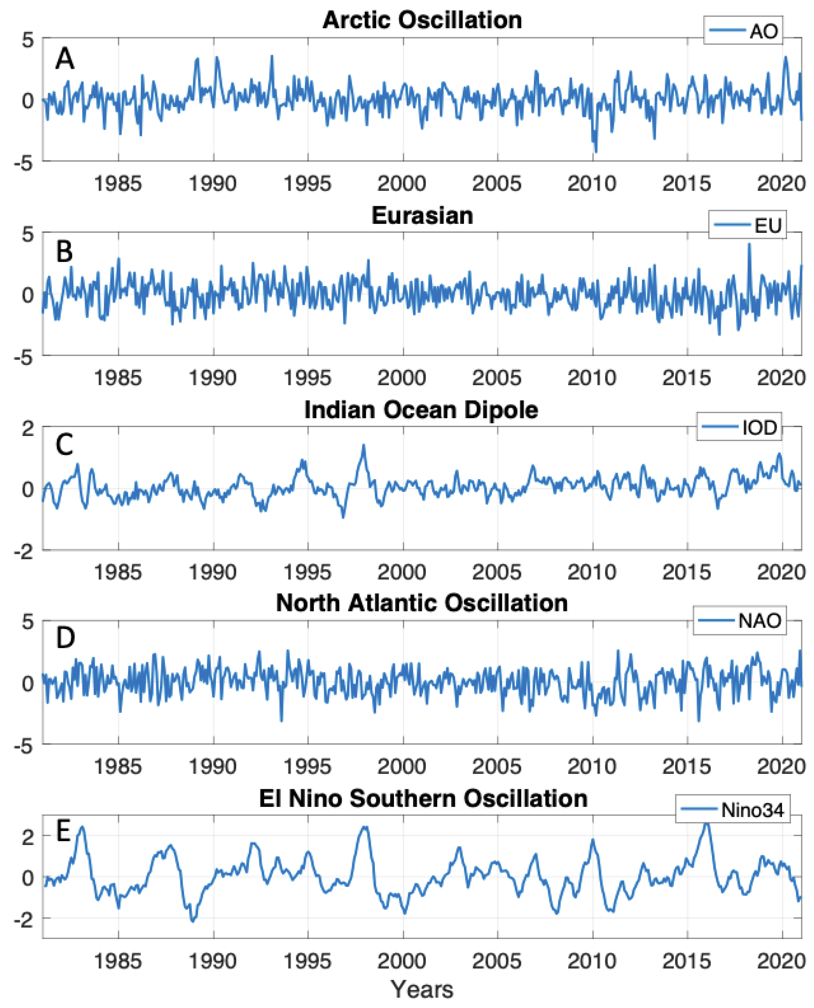
2.1. Modes of Variability

MoVs can affect global and regional climates on different spatial and temporal scales, have important impacts on human activities and ecosystems, and are a useful tool for simplifying the understanding of the climate system [20]. This section briefly describes each of the five MoVs investigated here. The monthly data used to represent the AO, Eurasian teleconnection, IOD, NAO, and Nino34 were obtained directly from the NOAA ESRL database (http://psl.noaa.gov/; accessed on 1 July 2021) for the period January 1981–December 2020. The five timelines are shown in Figure 1.
Figure 1. Global modes of variability (MoVs) investigated in this study, shown on a monthly timescale. The years explored for each index span from January 1981 to December 2020. The timelines shown above are the (A) Arctic Oscillation (AO), (B) Eurasian teleconnection, (C) Indian Ocean Dipole (IOD), (D) North Atlantic Oscillation (NAO), and (E) El Niño southern oscillation (Nino34).
Atmosphere 15 00142 g001
The AO is an oscillation of atmospheric pressure between the Arctic and the mid-latitudes of the North Pacific and North Atlantic. The AO is an important mode of climate variability for the Northern Hemisphere [21] because when the AO is strongly positive, a strong mid-latitude jet stream steers storms northward, reducing cold air outbreaks in the mid-latitudes, which can include the HMA region. The Eurasian teleconnection is one of the major MoVs in the Northern Hemisphere winter and features a mid-tropospheric, west–east-oriented wave train over Eurasia [22]. This pattern may be the most important mid-tropospheric teleconnection pattern of the interannual variations of the East Asian winter monsoon [23]. The IOD, also known as the Indian Niño, is an irregular oscillation of sea surface temperatures in which the western Indian Ocean becomes alternately warmer (positive phase) and then colder (negative phase) than the eastern part of the ocean. The IOD affects the strength of monsoons over the Indian subcontinent [24]. The NAO is a close relative of the AO [21] and is commonly defined as a weather phenomenon over the North Atlantic Ocean of fluctuations in the difference of atmospheric pressure at sea level between the Icelandic Low and the Azores High. It has been suggested that the NAO influences the strength and direction of westerly winds and the location of storm tracks across the North Atlantic [25]. The Nino34 (also commonly known as ENSO) is an episodic departure from expected sea surface temperatures in the equatorial Pacific Ocean [20]. These warmer or cooler-than-normal ocean temperatures can affect weather patterns around the world by influencing high- and low-pressure systems, winds, and precipitation. Nino34 is the largest source of interannual climate variability on a global scale and arises from interactions between the ocean and the atmosphere in the tropical Pacific [20], and may bring much-needed moisture to a region while causing extremes of too much or too little water in others.

2.2. Region of Focus

There are two regions of analysis in this study: a larger domain that covers 60 W–120 E and 5 S–90 N (Figure 2 and Figure 3) and a smaller domain that covers 65 E–105 E and 20 N-45 N (Figure 4, Figure 5, Figure 6, Figure 7, Figure 8 and Figure 9). The larger domain is used to examine spatial correlations between MoVs and the z250 data to investigate how large-scale atmospheric patterns affect the MoVs’ impact on weather and climate in HMA. This is because these large-scale patterns impact the HMA region from potentially 1000s of km away. The smaller domain is used to examine spatial correlations between MoVs and HMA climate variables, such as temperature, precipitation, and snow cover. We refer to HMA as the region that includes parts of China, Afghanistan, Pakistan, Nepal, India, Bangladesh, Myanmar, Kazakhstan, and Tajikistan and stretches across several mountain ranges, including the Himalayas, Hindu Kush, Karakoram, and Inner Tibetan Plateau.

2.3. MERRA-2

MERRA-2 is the dataset used for investigating the climate variables in this study. MERRA-2 is NASA’s most recent global atmospheric reanalysis product [19,26]. We obtained information from MERRA-2 on four variables for the period January 1981–December 2020. The first variable we obtained from MERRA-2 was the geopotential height at 250 hPa (H250 from the “Single-Level Diagnostics” collection; GMAO 2015a), referred to as z250 for the remainder of this paper. The second variable obtained from MERRA-2 was 2 m air temperature (T2M from the “Single-Level Diagnostics” collection [27]). The third variable obtained from MERRA-2 was total precipitation (PRECTOT from the “Surface Flux Diagnostics” collection; [28]); however, MERRA-2 uses observation-based precipitation data as forcing for the land surface parameterization [29], and the precipitation forcing data derived from this approach are archived as the output variable called PRECTOTCORR, which is available as part of the “Surface Flux Diagnostics” collection [28]. For our analysis, we used the PRECTOTCORR variable, and refer to it as PRECTOT for the remainder of this paper. The final variable obtained from MERRA-2 was snow cover area fraction (FRSNO from the “Land Surface Diagnostics” collection and called fSCA for the remainder of this paper; [30]). It is important to note that the spatial resolution of the MERRA-2 data (~0.5 degrees) can be sufficient to capture medium-to-large-scale features, but are not adequate to resolve fine-scale features that can be present in the complex topography of the HMA region. Yet, we chose MERRA-2 as the dataset to investigate the climate variables because it provides spatially and temporally consistent information that other forms of data may not provide (e.g., see Massoud et al., 2023 [18] on data coverage for the HMA region).

2.4. Correlation Tests

The relationships between the MoVs and the climate data examined in this study were first calculated as the correlation of the long-term vector of each mode of climate variability (monthly data from January 1981 to December 2020, as shown in Figure 1) with the time vector in each grid cell of the climate variables of interest. Correlations were estimated using the “corr” function in MATLAB (www.mathworks.com/help/stats/corr.html [31]; accessed on 1 July 2021). In Figure 2 and Figure 3, the anomalies of the z250 data are estimated to calculate this correlation. The anomalies were estimated by removing the monthly climatology (i.e., the long-term mean value for each calendar month throughout the length of the available data record). For the remainder of the results, grids with less than 90% confidence (estimated through the “corr” function p-value output) are masked out in these figures so that the shown colors in Figure 2, Figure 3, Figure 4, Figure 5, Figure 6, Figure 7, Figure 8 and Figure 9 only display regions that were significantly correlated. In these figures, red indicates a positive correlation and blue depicts a negative correlation.
To investigate if there were any time lags that showed a higher level of correlation between an MoV and the climate data, we also applied a time-shift on the data and tested for lagged cross-correlations between the MoV at time t and the climate variables at time t+lag (and t-lag), where lag is the number of months that were shifted for the correlation analysis. This can explain, for example, how well the IOD value in December can help predict T2M in June, how well the Nino34 value in July can predict PRECTOT one year later, or how well the fSCA in December can help predict the Eurasian teleconnection in March. To do this, we used the “xcorr” function in MATLAB (https://www.mathworks.com/help/matlab/ref/xcorr.html; accessed on 1 July 2021), which is similar to the “corr” function but applies a moving window for the time lag and computes a lagged cross-correlation for each time window. We set a maximum time lag of 6 months to check for any lagged relationships that may be present in the data. To generate a timeline for each climate variable that can be used in the time-lagged cross-correlation test with the MoV data, a spatial average of the whole domain was used for each climate variable at each time step.

3. Results

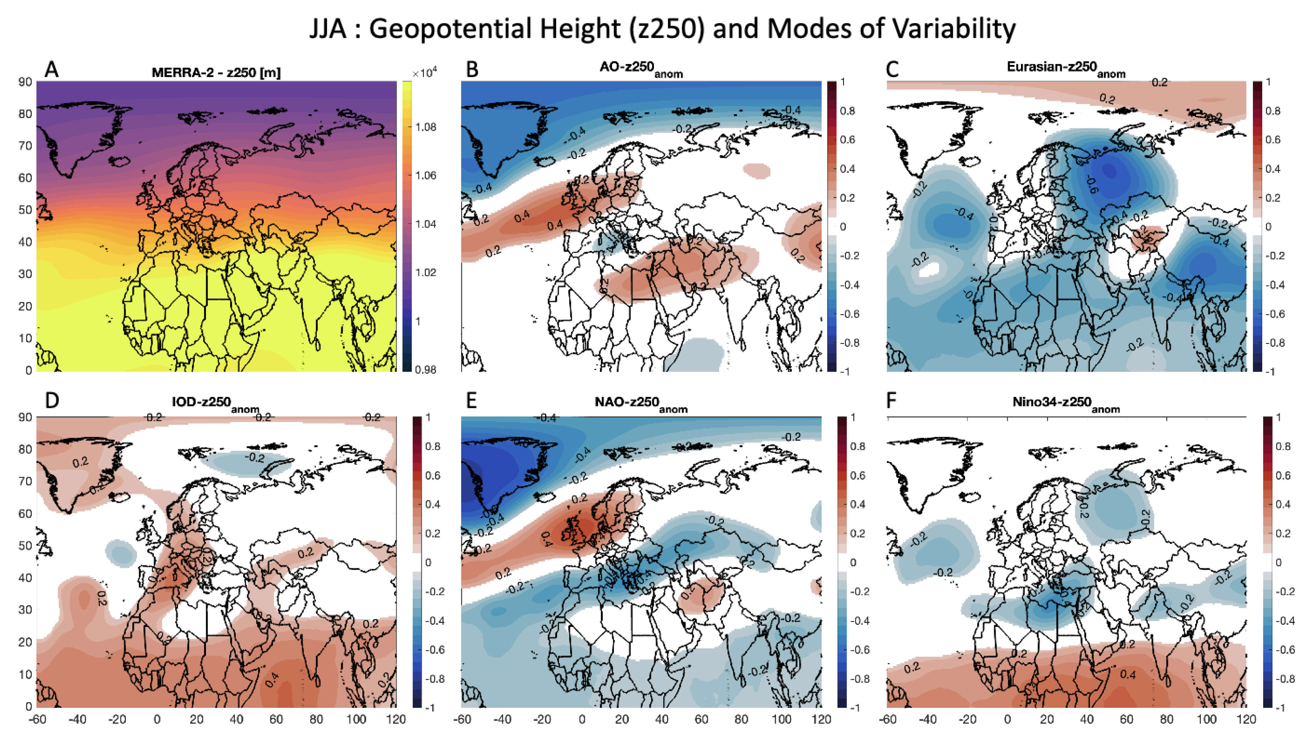
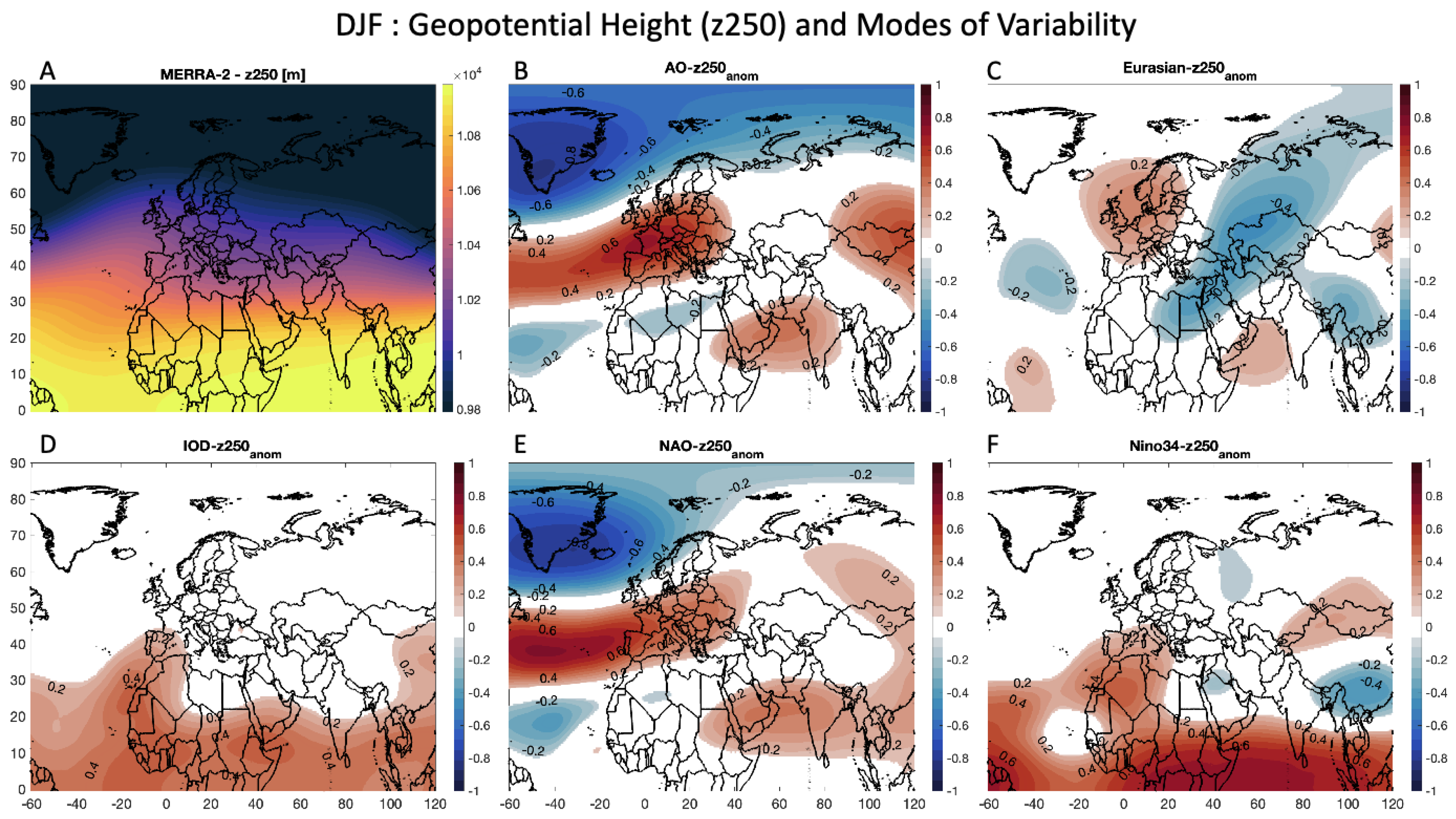
3.1. Correlating Modes of Climate Variability with Geopotential Height (z250)

The results in this paper are split up by season, and we separate the correlation analysis for the winter (DJF) and summer (JJA) seasons. Figure 2 and Figure 3 display the results for the z250 data. In Figure 2A, information on mean wintertime z250 is shown, with high latitudes (e.g., 40° N and higher) showing lower geopotential height values of less than 10,000 m (or 10 km) and tropical latitudes showing values close to 11,000 m (or 11 km). When estimating the correlation in each grid cell to the MoV data from Figure 1, different regions emerged as potentially having a significant relationship. Figure 2B shows the correlation between the AO and z250 anomalies, and the region spanning the Arctic Ocean and Greenland shows a significant negative correlation (lower than −0.2 in most regions and lower than −0.6 over Greenland). There is also a region that spans from the North Atlantic through most of Europe (greater than 0.6 in some regions) and a region in Eastern Asia (greater than 0.4) that show a pattern of positive correlation between the AO and z250 anomalies in the winter. Figure 2C shows the correlation between the Eurasian teleconnection and z250 anomalies in the winter, and, again, the region over Europe has a positive correlation (greater than 0.2). There is also a broad region spanning Russia, the Middle East, and parts of North Africa that have a negative correlation (less than −0.4) between the Eurasian teleconnection and the z250 anomalies. Figure 2D shows the correlation between the IOD and z250 anomalies in the winter, with all regions in the tropics having a positive correlation (greater than 0.4). The relationship of wintertime NAO to z250 (Figure 2E) shows a very similar pattern to that of the AO (Figure 2A), and the relationship of wintertime Nino34 to z250 (Figure 2F) shows a very similar pattern to that of the IOD (Figure 2D), with the only exception being in the southeast Asia region, where a negative correlation was found (as low as −0.4).
Figure 2. Wintertime (DJF) relationship between the various MoVs explored in this study and geopotential height. (A) DJF geopotential height at 250 hPa (z250) from MERRA-2, with units [m]. Correlation of DJF z250 with the (B) AO, (C) Eurasian teleconnection, (D) IOD, (E) NAO, and (F) Nino34 at each grid cell. Grids with less than 90% confidence are masked out in these figures. Red indicates a positive correlation and blue depicts a negative correlation.
Atmosphere 15 00142 g002
Figure 3A shows information on mean summertime z250, with high latitudes (e.g., 40° N and higher) again showing lower geopotential height values of just slightly over 10,000 m (or 10 km) and tropical latitudes showing values higher than 11,000 m (or 11 km). Summertime z250 values were consistently higher than those in the winter. When looking at the correlation of summertime z250 anomalies with the MoVs (Figure 3B–F), many of the relationships are very similar to those shown for the wintertime in Figure 2. For example, the AO (Figure 3B) and NAO (Figure 3E) show roughly an identical pattern to their counterparts in Figure 2B,E, except for a northward shift in the positive correlation seen over Europe and a band of negative correlation between the NAO and z250 anomalies stretching from the Atlantic through southern Europe and into central Asia (Figure 3E). The relationship for the IOD (Figure 3D) is also very similar to its counterpart in Figure 2, with positive values seen throughout the globe and with an extension of positive relationships throughout Europe and over Greenland (greater than 0.2). The relationship with the Eurasian teleconnection (Figure 3C) is mostly negative throughout the domain, with a peak over western Russia (less than −0.6). For Nino34 (Figure 3F), the tropical latitudes have a positive correlation (greater than 0.4), with various regions having negative correlations (e.g., North Atlantic, Mediterranean Sea, West Russia, and East Asia).
Figure 3. Like Figure 2, but for the summertime (JJA) geopotential height at 250 hPa (z250).
Atmosphere 15 00142 g003

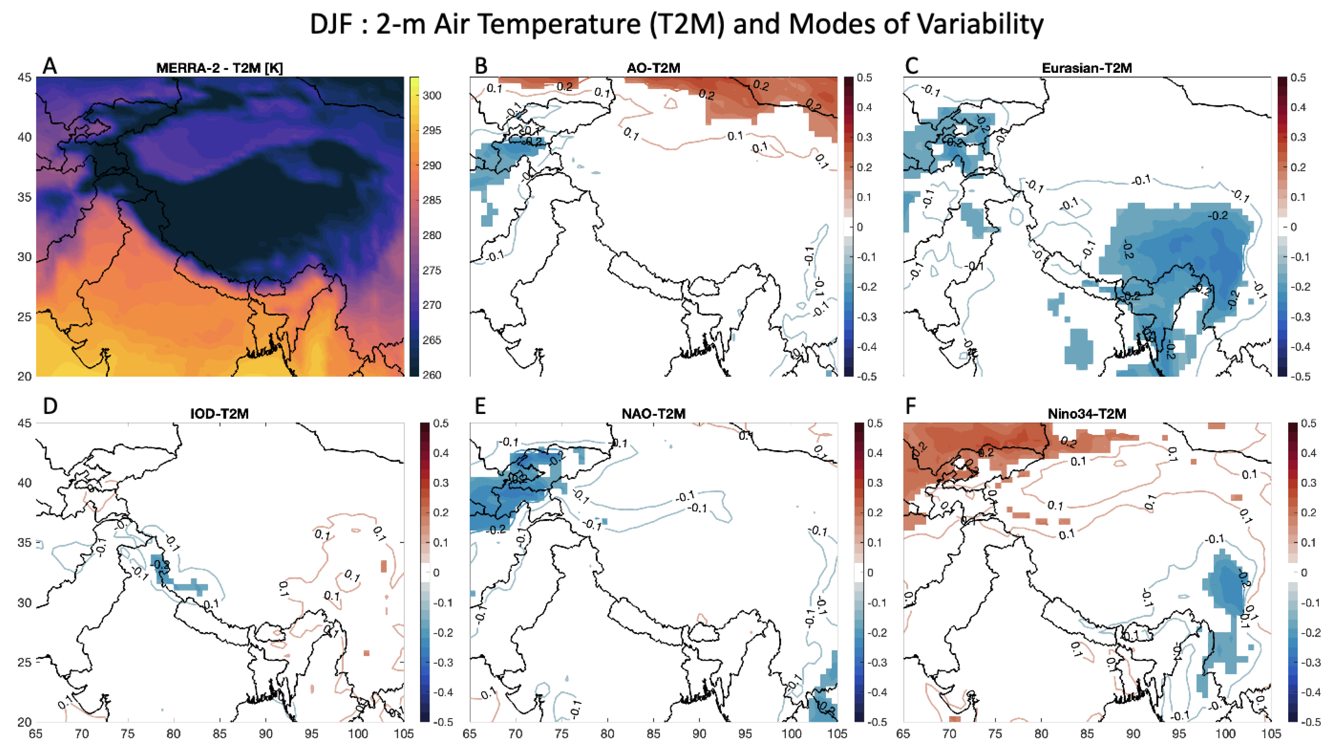
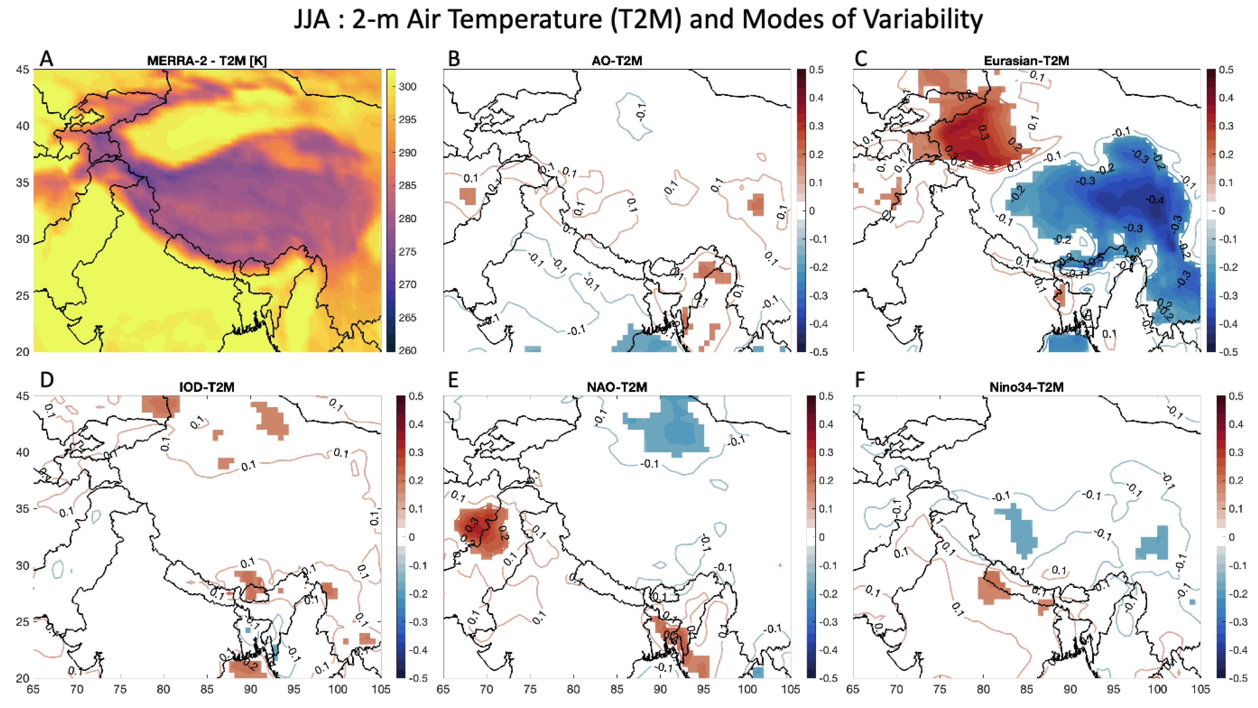
3.2. Correlating Modes of Climate Variability with Temperature (T2M)

Figure 4 and Figure 5 display the results for the T2M over the HMA region. In Figure 4A, information on mean wintertime T2M data is shown, with high altitudes (e.g., mountain ranges and the Inner Tibetan Plateau) exhibiting temperatures that are below freezing and regions with low elevation (e.g., the Indian subcontinent) having higher temperatures of up to 295 K. When determining the correlation in each grid cell to each MoV, no noticeable regions emerged as potentially having a significant relationship with the IOD (Figure 4D). For the AO (Figure 4B), Eurasian teleconnection (Figure 4C), and NAO (Figure 4E), there is a negative correlation with wintertime T2M (less than −0.2) in the Hindu Kush, the mountainous regions near Afghanistan. For the Eurasian teleconnection (Figure 4C), there is also a region of negative correlation in the Inner Tibetan Plateau and East India (less than −0.2). For Nino34 (Figure 4F), there is a region of positive correlation in the northwest portion of the domain (higher than 0.2) and a small region of negative correlation in central China (less than −0.2).
Figure 5A shows information on mean summertime T2M in HMA, again with high altitudes exhibiting temperatures that are close to freezing and regions with low elevation having temperatures higher than 300 K. The AO (Figure 5B), IOD (Figure 5D), and Nino34 (Figure 5F) show no significant relationship with summertime T2M in HMA. However, the Eurasian teleconnection (Figure 5C) shows a strong dipole, with regions near western China having a positive correlation (greater than 0.3) and a large portion of the Inner Tibetan Plateau and South China having a negative correlation (less than −0.4). The NAO (Figure 5E) plot shows small regions between Afghanistan and Pakistan and in Bangladesh that have positive correlations (greater than 0.3).
Figure 4. Wintertime (DJF) relationship between the various MoVs explored in this study and 2 m air temperature (T2M). (A) DJF T2M from MERRA-2, with units [K]. Correlation of DJF T2M with the (B) AO, (C) Eurasian teleconnection, (D) IOD, (E) NAO, and (F) Nino34 at each grid cell. Grids with less than 90% confidence are masked out. Red indicates a positive correlation and blue depicts a negative correlation.
Atmosphere 15 00142 g004
Figure 5. Like Figure 4, but for summertime (JJA) 2 m air temperature (T2M).
Atmosphere 15 00142 g005

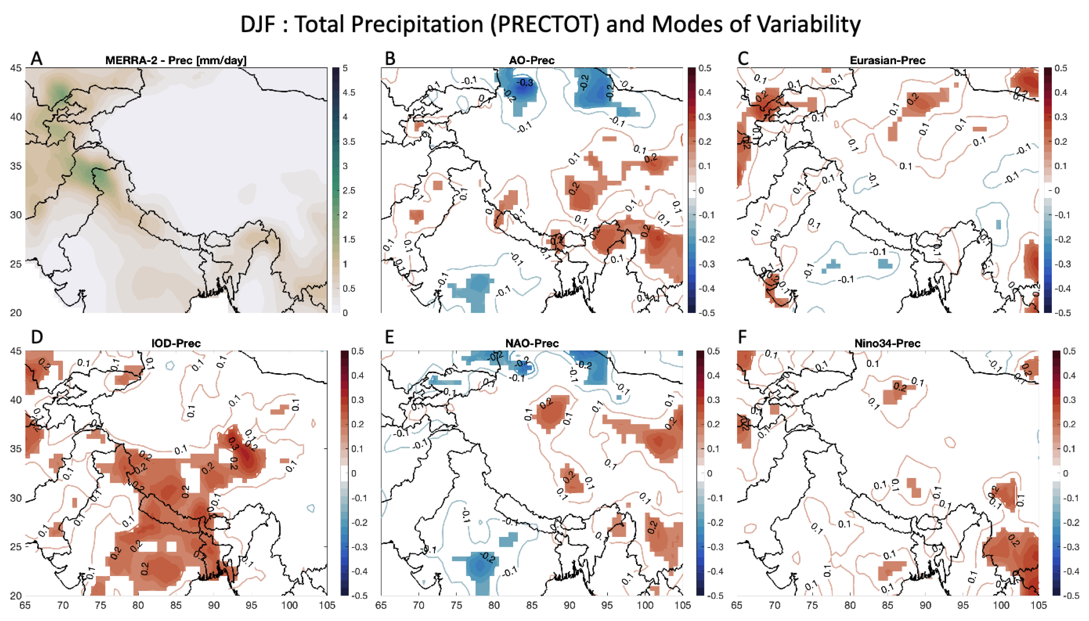
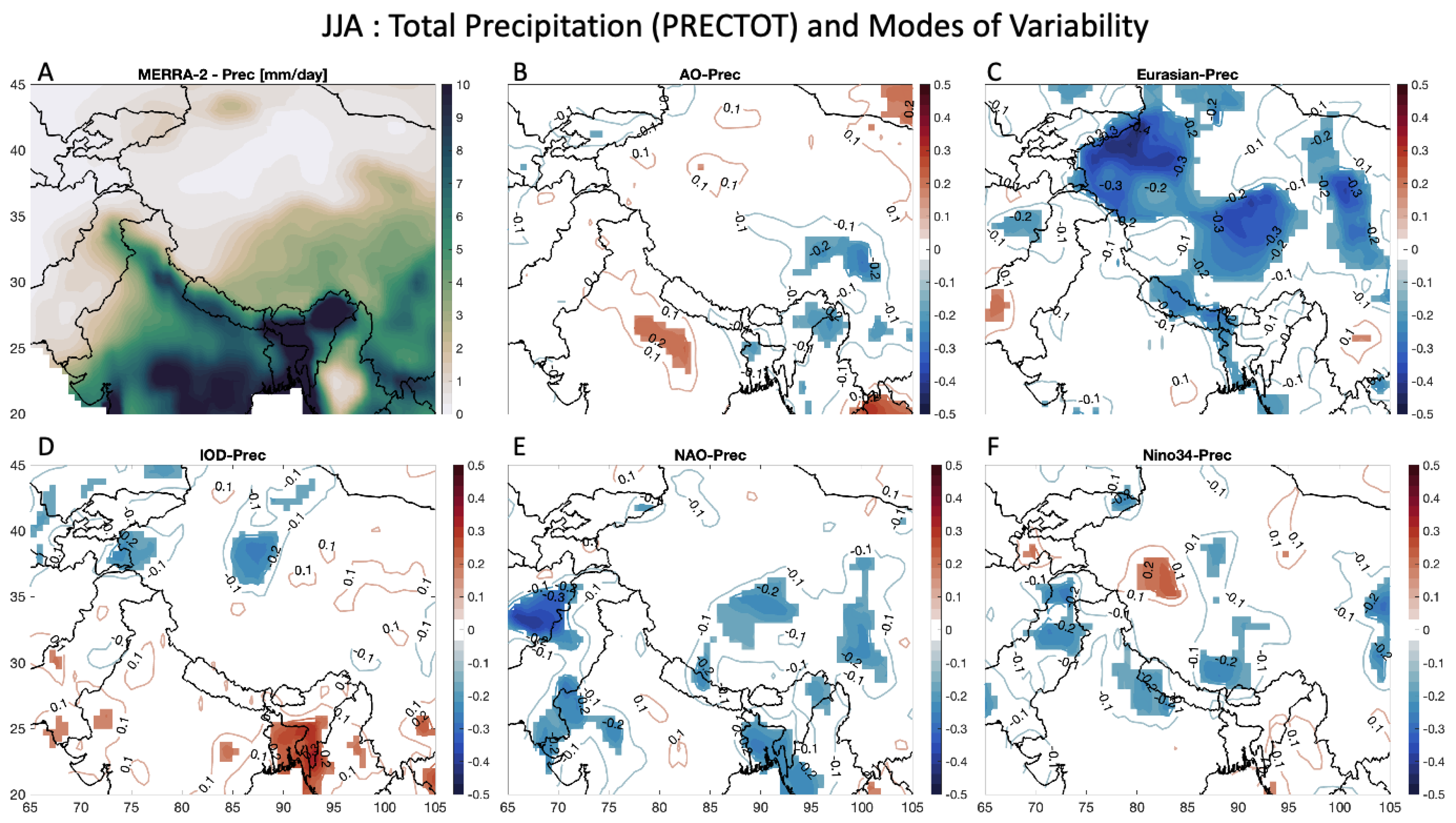
3.3. Correlating Modes of Climate Variability with Precipitation (PRECTOT)

Figure 6 and Figure 7 display the results for the PRECTOT over the HMA region. In Figure 6A, information on mean wintertime PRECTOT data is shown, with regions with high topographic variability (e.g., Hindu Kush and Karakoram) exhibiting slightly higher precipitation rates of up to 5 mm/day and the remainder of the domain showing values of less than 1 mm/day. When determining the correlation in each grid cell to each MoV, no noticeable regions emerged as potentially having a significant relationship with the Eurasian teleconnection (Figure 6C) or Nino34 (Figure 6F), except for a few regions throughout the domain that show a positive correlation (e.g., South China for Nino34). For the AO (Figure 6B) and NAO (Figure 6E), the patterns are very similar, with some regions in China having positive correlations (greater than 0.2) and some regions in North China and India having negative correlations (as low as −0.3). For the IOD (Figure 6D), there is a broad region through India and western China (and through the Himalayan mountain range) that has a positive correlation (up to 0.3).
Figure 6. Wintertime (DJF) relationship between the various MoVs explored in this study and total precipitation (PRECTOT). (A) DJF PRECTOT from MERRA-2, with units [mm/day]. Correlation of DJF PRECTOT with the (B) AO, (C) Eurasian teleconnection, (D) IOD, (E) NAO, and (F) Nino34 at each grid cell. Grids with less than 90% confidence are masked out. Red indicates a positive correlation and blue depicts a negative correlation.
Atmosphere 15 00142 g006
Figure 7A shows information on mean summertime PRECTOT in HMA, with much higher precipitation rates shown in the domain compared to the wintertime, mostly due to the impacts of the Indian summer monsoon. Some regions in the Indian subcontinent experience precipitation rates higher than 10 mm/day in the summer (Figure 7A), with many other parts of the domain seeing rates as high as 5 mm/day. When estimating the relationship of summertime PRECTOT with the MoVs, most relationships are significantly negative, such as that with the Eurasian teleconnection (Figure 7C), which has a negative correlation pattern in most of western China and the Himalayas (as low as −0.4). The other indices have many smaller regions with negative correlation patterns, such as the NAO (Figure 7E) and Nino34 (Figure 7F). There are also small positive correlation patterns seen for the AO (Figure 7B) in India (higher than 0.2) and for the IOD (Figure 7D) in Bangladesh (higher than 0.3).
Figure 7. Like Figure 6, but for summertime (JJA) total precipitation (PRECTOT). Note: The maximum value of PRECTOT in Figure 7A is just over 10 mm/day.
Atmosphere 15 00142 g007

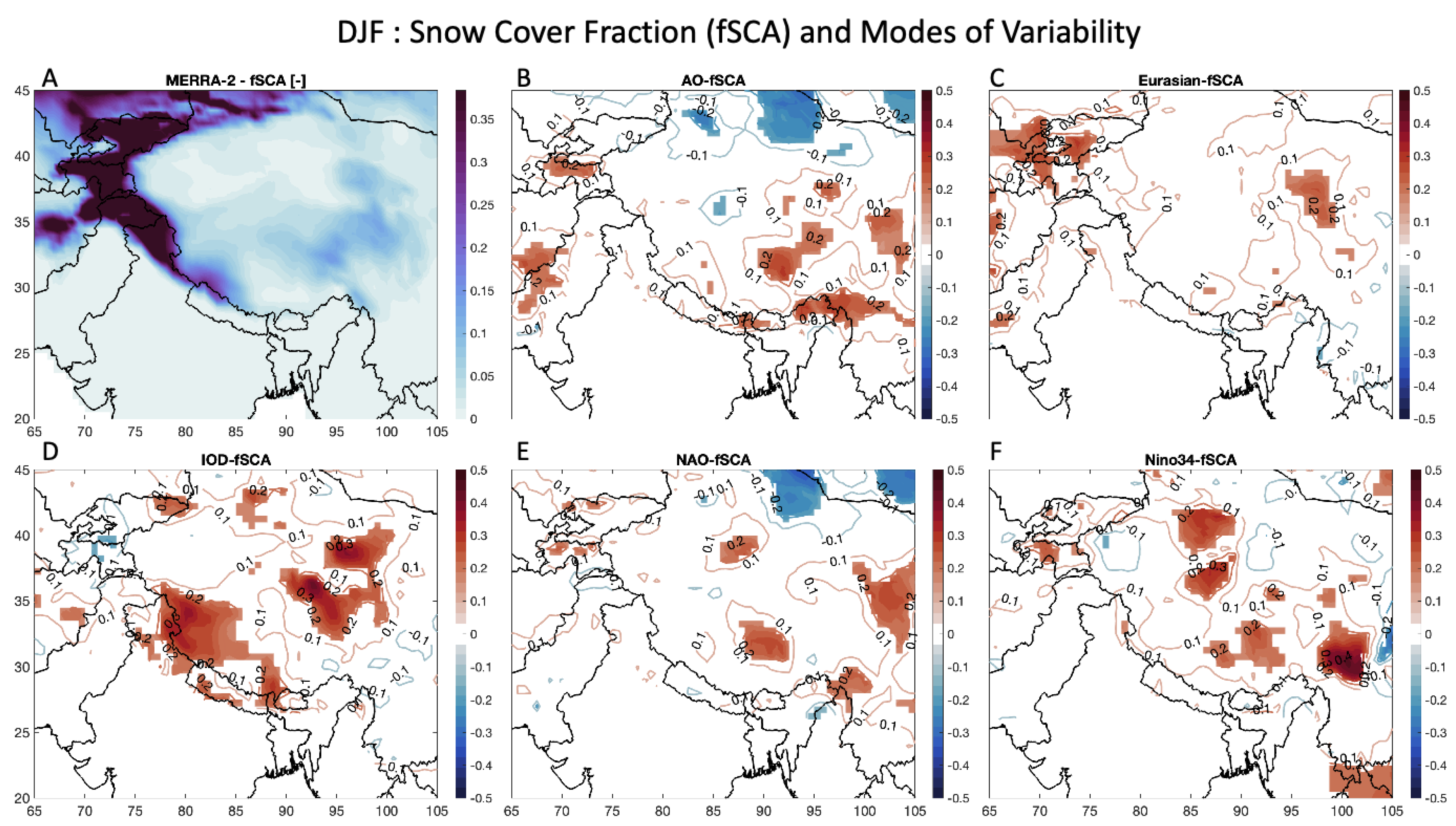
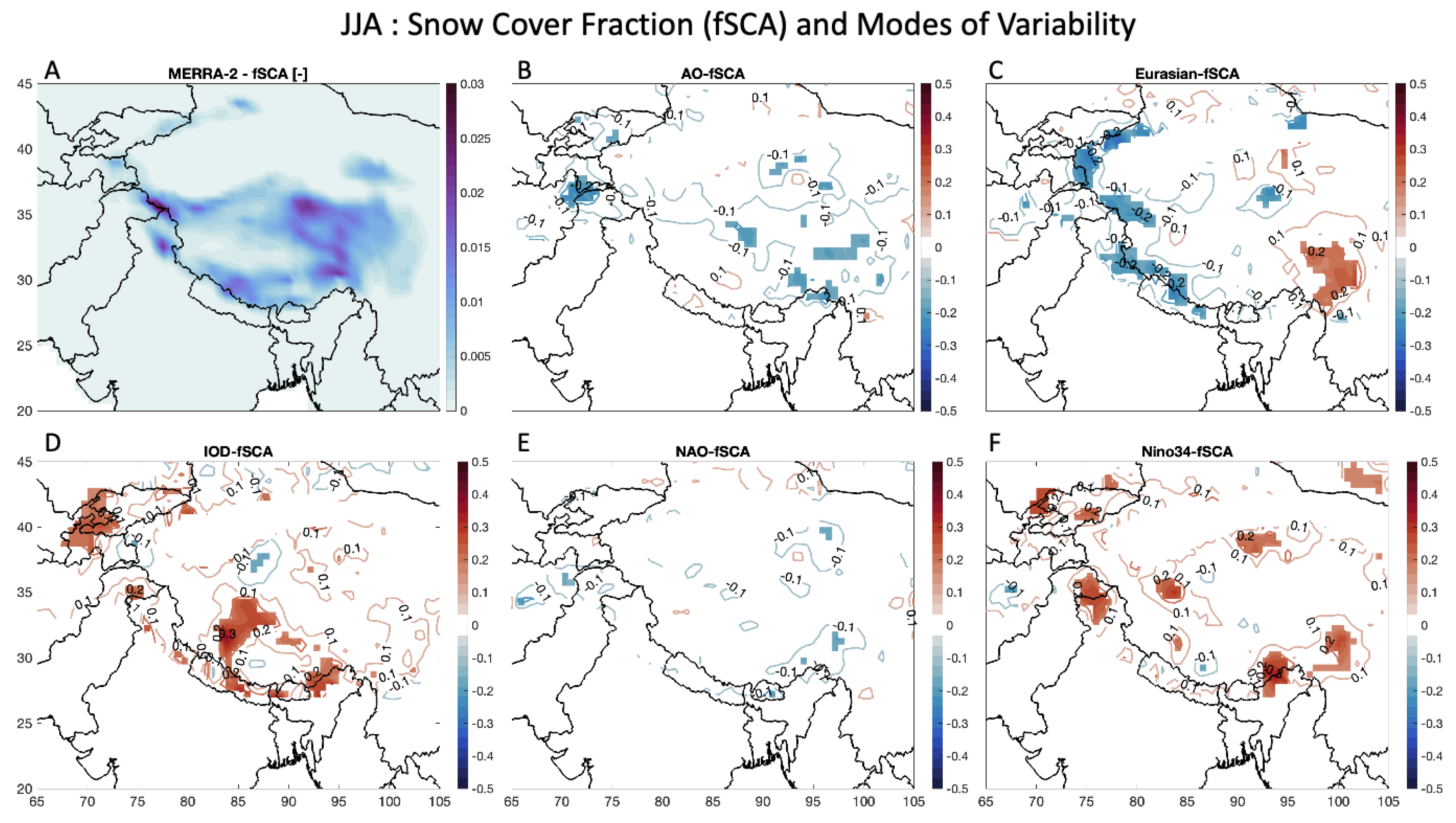
3.4. Correlating Modes of Climate Variability with Fractional Snow Cover Area (fSCA)

Figure 8 and Figure 9 display the results for fSCA over the HMA region. In Figure 8A, information on mean wintertime fSCA data is shown, and regions with high elevation are shown to have noticeable fSCA values, with regions of high topographic variability (e.g., Hindu Kush and Karakoram) exhibiting the highest fSCA values (e.g., greater than 0.35 and in some locations up to 1). When determining the correlation in each grid cell to each MoV, no noticeable regions emerged as having a significant relationship with the Eurasian teleconnection (Figure 8C), except for small regions of positive correlation, e.g., the northwest part of the domain (higher than 0.2). For the other indices, many regions of positive correlations are shown, such as for the IOD (Figure 8D) in the Himalayas and central China (higher than 0.3) and other various regions for the AO (Figure 8B), NAO (Figure 8E), and Nino34 (Figure 8F), such as in China (higher than 0.4).
Figure 9A shows information on mean summertime fSCA in HMA, with much lower snow cover shown in the domain compared to the wintertime, mostly due to the higher temperatures experienced in the summer. Some regions in the Himalayas and Inner Tibetan Plateau experience fSCA higher than 0.02 in the summer (Figure 9A), with the remainder of the domain seeing close to 0 snow cover area. When estimating the relationship of summertime fSCA with the MoVs, no noticeable regions emerged as potentially having a significant relationship with the AO (Figure 9B) or NAO (Figure 9E), except for the AO, which has a small region of negative correlation in the Hindu Kush region (lower than −0.2). The Eurasian teleconnection (Figure 9C) has different regions of negative correlation (as low as −0.2), such as in the Himalayas and the Karakoram, and a region of positive correlation (higher than 0.2) near central China. For the IOD (Figure 9D) and Nino34 (Figure 9F), there are some regions with positive correlation (as high as 0.3) throughout HMA, such as the Himalayas for the IOD and the Karakoram for Nino34.
Figure 8. Wintertime (DJF) relationship between the various MoVs explored in this study and fractional snow cover area (fSCA). (A) DJF fSCA from MERRA-2, with no units [-]. Correlation of DJF fSCA with the (B) AO, (C) Eurasian teleconnection, (D) IOD, (E) NAO, and (F) Nino34 at each grid cell. Grids with less than 90% confidence are masked out. Red indicates a positive correlation and blue depicts a negative correlation.
Atmosphere 15 00142 g008
Figure 9. Like Figure 8, but for summertime (JJA) fractional snow cover area (fSCA).
Atmosphere 15 00142 g009

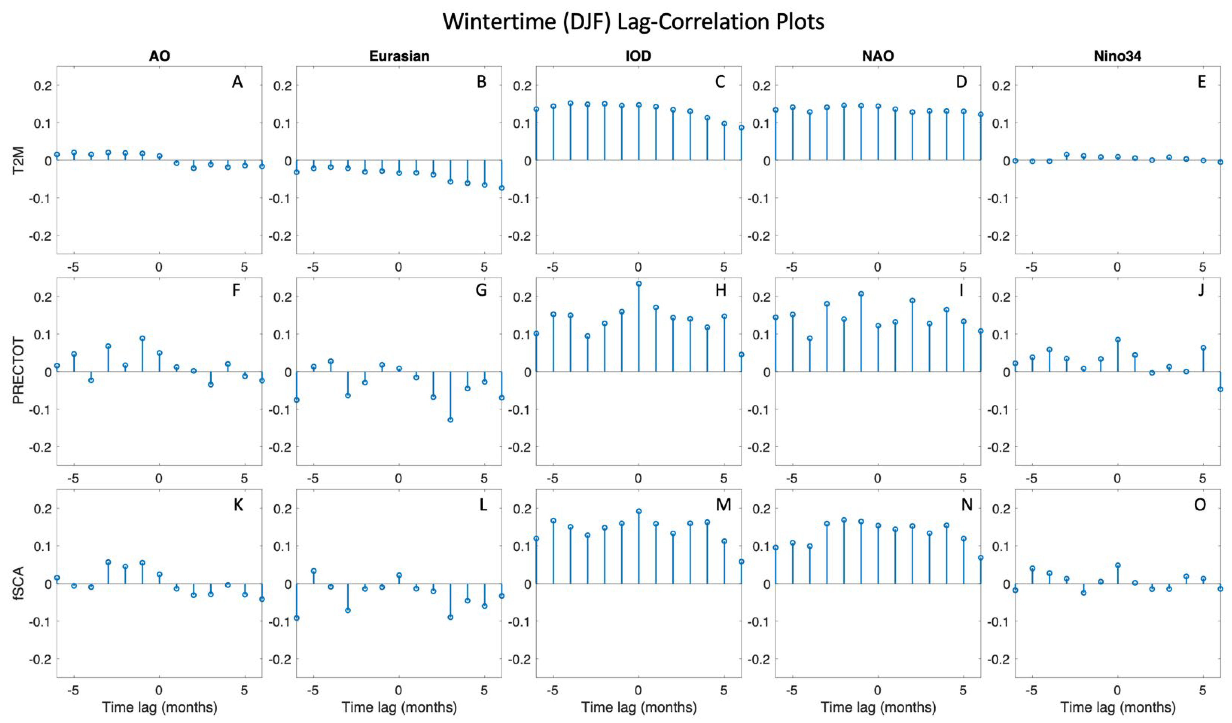
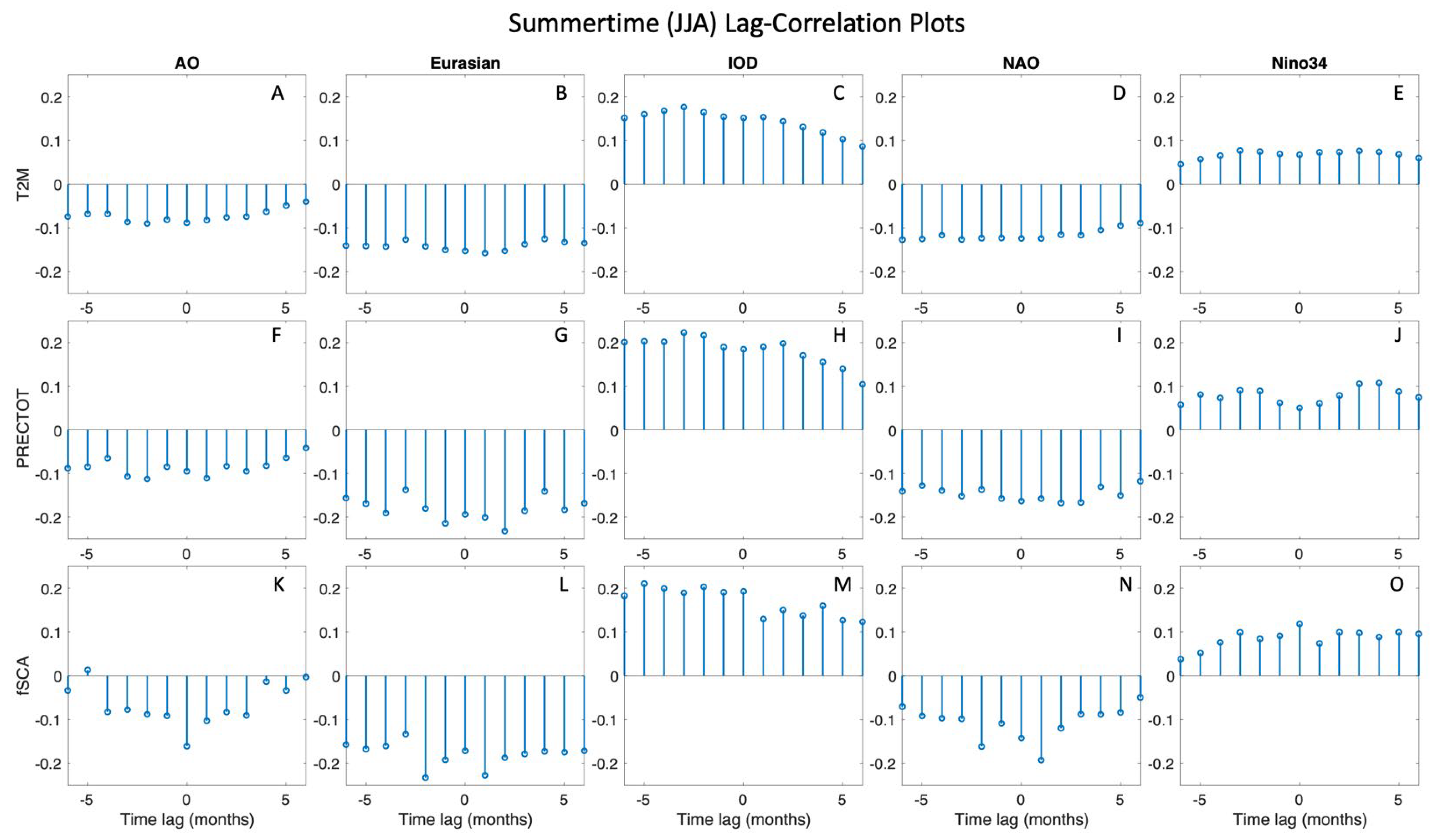
3.5. Time-Lagged Cross-Correlation of MoVs with Climate Variables

Figure 10 shows the results from the time-lagged cross-correlation analysis of the MoVs with the spatially averaged climate variable timelines during the winter (DJF) months. These figures show the strength of the signal at each time window. A peak in the negative time lag can indicate that knowing the MoV can help predict the climate variable, whereas a peak in the positive time lag can indicate that knowing the climate variable can help predict the MoV. For T2M during the winter (Figure 10A–E), the lagged cross-correlation with the AO, Eurasian, and Nino34 data did not show any strong correlations, whereas for the IOD and NAO, there is a low-to-moderate correlation, with a peak of ~0.15 at the 0-month mark. Similar patterns can be seen for the relationships of the MoVs with wintertime precipitation (Figure 10F–J) and snow cover (Figure 10 K–O), with peak correlations of ~0.2 at the 0-month mark. This positive lagged cross-correlation between the IOD and NAO and the climate variables can indicate that higher T2M, PRECTOT, and fSCA can be expected on average in the HMA region whenever the IOD and NAO are in the positive phases in the winter. These results reinforce those shown in Figure 6 and Figure 8.
Figure 10. Winter (DJF) time-lag cross-correlation plots for each MoV and climate variable pair are shown here. The spatial means of the climate variables were taken at each time step and used for this analysis. At a time lag of 0, the value shows the lagged cross-correlation between the MoV and the climate variable at the same time steps (0 lag). For negative time lags, the value shows the lagged cross-correlation between the MoV prior to the timestep of the climate variable (e.g., lagged cross-correlation between AO at time t and T2M at time t+lag). For positive time lags, the value shows the lagged cross-correlation between the MoV after the timestep of the climate variable (e.g., lagged cross-correlation between AO at time t+lag and T2M at time t). The maximum time lag analyzed in this plot is 6 months (AO).
Atmosphere 15 00142 g010
Figure 11 shows the results from the time-lagged cross-correlation analysis of the MoVs with the spatially averaged climate variable timelines during the summer (JJA) months. In the summertime (Figure 11), there seems to be more predictability than in the winter (Figure 10). For T2M during the summer (Figure 11A–E), the lagged cross-correlation with the AO, Eurasian teleconnection, and NAO had negative relationships, whereas the correlations with the IOD and Nino34 had positive relationships, with peaks at the 0-month mark of nearly −0.2 and +0.2, respectively. Very similar results can be seen for summertime precipitation (Figure 11F–J) and snow cover (Figure 11K–O). This positive lagged cross-correlation between the IOD and Nino34 and the climate variables can indicate that higher T2M, PRECTOT, and fSCA can be expected on average in the HMA region whenever the IOD and Nino34 are in the positive phases in the summer. The opposite can be expected for the AO, Eurasian teleconnection, and NAO, where lower T2M, PRECTOT, and fSCA can be expected on average in the HMA region whenever these MoVs are positive in the summer. These results reinforce those shown in Figure 5, Figure 7 and Figure 9.
Figure 11. Same as in Figure 10, but for summer (JJA) time-lag cross-correlation results (AO).
Atmosphere 15 00142 g011

4. Discussion

4.1. Implications of Evident Correlations between MoVs and Climate in HMA

In this section, we aim to answer some of the questions regarding the search for evidence that shows relationships between the considered MoVs and climate variables in HMA. If any relationships exist, this work also searches for specific regions that exhibit significant correlations. If this is found, we aim to explore the implications of these relationships for both scientific understanding as well as for predictability.
To this end, there are some obvious patterns and relationships that emerge. For example, Figure 4 shows the relationship between wintertime T2M and the MoVs explored in this study, and the mountain ranges just north of Afghanistan, also known as the Karakoram and Hindu Kush regions, show a significant negative correlation for the AO (Figure 4B), Eurasian teleconnection (Figure 4C), and NAO (Figure 4E). This is also shown for a large region in central China and eastern India for the Eurasian teleconnection. This implies that when either the AO, Eurasian teleconnection, or NAO is in the positive phase of their oscillation, colder temperatures can be expected in these regions of HMA in the winter. As for summertime T2M, a similar finding can be seen in Figure 5C, which shows a significant negative correlation with the Eurasian teleconnection in the Inner Tibetan Plateau and central and southern China, but a significant positive correlation in northwestern China. This finding suggests that when the Eurasian teleconnection is in the positive (negative) phase of its oscillation, colder temperatures can be expected in the Inner Tibetan Plateau and central China (northwestern China) in the summer.
For exploring relationships between MoVs and wintertime precipitation in HMA, Figure 6 shows that there are some regions that have a significant positive correlation with the IOD (Figure 6D), such as India, the Himalayas, and the Inner Tibet Plateau. Furthermore, the remaining MoVs also have a positive correlation with wintertime precipitation in various regions, especially some regions within China for the AO (Figure 6B) and NAO (Figure 6E). In India, however, there is a region that shows a negative correlation with the AO and NAO. These results imply that when any of the MoVs are in the positive phase of their oscillation, especially the IOD, wetter conditions can be expected in most of the HMA region in the winter. For summertime precipitation (Figure 7), there are mostly negative correlations with the MoVs, especially the Eurasian teleconnection (Figure 7C). This indicates that when the MoVs are in their positive phase in the summer, drier conditions can be expected in different parts of HMA. The exception here is shown in the Indian subcontinent, where summertime PRECTOT has a significant positive correlation with the AO (Figure 7B) and IOD (Figure 7D).
As for the relationships between MoVs and wintertime fSCA in HMA, Figure 8 shows evidence of similar relationships as those shown for wintertime precipitation in Figure 6. That is, some regions have a significant positive correlation with the IOD (Figure 8D), such as the Himalayas and Inner Tibet Plateau, and the remaining MoVs also have a positive correlation with wintertime fSCA in various regions, especially some regions in the Karakoram and within China for the AO (Figure 8B), Eurasian teleconnection (Figure 8C), NAO (Figure 8E), and Nino34 (Figure 8F). These results highlight similar patterns as those for wintertime precipitation, which imply that when any of the MoVs are in the positive phase of their oscillation, especially the IOD, more snow cover can be expected in most of the HMA region in the winter. For summertime fSCA (Figure 9) in HMA, there are rare clear relationships that emerge in our study that exhibit any patterns or significant correlations, except for the Eurasian teleconnection (Figure 9C), which shows a negative correlation in the Himalayas, and the IOD (Figure 9D) and Nino34 (Figure 9F), which show a positive correlation in some parts of HMA, indicating that there could be some predictability of summertime snow cover in these regions associated with the Eurasian teleconnection, IOD, or Nino34.

4.2. Connecting Results to Previous Findings and Underlying Physical Mechanisms

When the AO is strongly positive, a strong, mid-latitude jet stream steers storms northward, reducing cold air outbreaks in the mid-latitudes [21]. This is confirmed by our results in Figure 2B and Figure 3B, which show a northward shift of a positive correlation pattern between the AO and z250 between winter and summer over Europe. Figure 4B and Figure 6B also confirm this, with regions in the northernmost part of the domain showing a positive correlation between the AO and wintertime temperature and a negative correlation with precipitation. This may be explained by the AO being characterized by non-seasonal, sea-level pressure anomalies of one sign in the Arctic balanced by anomalies of the opposite sign centered at about 37–45° N [21]. When the AO index is positive, surface pressure is high in the polar region. This helps the middle latitude jet stream to blow strongly and consistently from west to east, thus keeping cold Arctic air locked in the polar region. When the AO index is negative, there tends to be low pressure in the polar region, weaker zonal winds, and greater movement of frigid polar air into middle latitudes [21].
For the Eurasian teleconnection, the results in Figure 5C, Figure 7C, and Figure 9C show positive correlations with temperatures and negative correlations with precipitation and snow cover in the summer in western China, near the Hindu Kush and Karakoram regions. Therefore, in this region, we find that the positive phase of the Eurasian teleconnection may cause higher temperatures as well as less rainfall, which results in less overall snow cover in the summer. These results reinforce previous findings that state that the Eurasian teleconnection explains up to 20% of the interannual variance of surface temperature over East Asia and that the positive phase of the Eurasian teleconnection produces less precipitation over eastern and central Asia [22].
When the IOD is in the positive phase, sea-surface temperatures and precipitation in the western Indian Ocean region are higher than normal, with a corresponding cooling of waters in the eastern Indian Ocean [24]. When the IOD is in the negative phase, the opposite conditions occur, with warmer water and greater precipitation in the eastern Indian Ocean and cooler and drier conditions in the west. Our results extend the understanding of the IOD’s impact on weather and climate in HMA, and Figure 4D, Figure 6D, and Figure 8D indicate that when the IOD is in the positive phase, there are lower temperatures as well as higher precipitation rates that result in a higher snow cover area in HMA in the winter.
For the NAO, like the AO, a positive phase can cause mid-latitude jet streams to shift northward, reducing precipitation rates and decreasing cold air outbreaks, which, in turn, causes higher temperatures. Our results show that a positive NAO phase in the winter can result in lower temperatures over some parts of HMA, such as the Hindu Kush region (Figure 4E), and a positive phase in the summer can result in higher temperatures and lower precipitation rates in this region (Figure 5E and Figure 7E), which can lead to lower snow cover (Figure 9E) in this region. This can be explained by the fact that westerly winds blowing across the Atlantic bring moist air into Europe and, in years when westerlies are strong, summers are cooler, winters are mild, and rain is frequent [32]. If westerlies are suppressed, the temperature is more extreme in summer and winter, leading to heat waves, deep freezes, and reduced rainfall. However, these correlations for the NAO are generally higher for regions in Europe [32] compared to the results reported here for the HMA region.
A positive Nino34, or the El Niño phase, coincides with colder temperatures in the southeast and warmer temperatures in the northwest parts of the domain in the winter (Figure 4F) and can be related to warmer conditions over India and cooler conditions in the Karakoram and Inner Tibetan Plateau in the summer (Figure 5F). Our results show evidence that during the El Niño phase, wetter conditions can be expected in the winter (Figure 6F), which can result in more snow cover (Figure 8F), and drier conditions are expected in the summer (Figure 7F); yet, higher amounts of snow cover (Figure 9F) could be due to the cooler temperatures (Figure 5F), which could result in more precipitation falling as snow or less overall snowmelt. Our results match those reported in [2], which showed that the positive phases of Nino34 have been shown to increase precipitation in the western Himalayan region during the winter, attributed to increased convergence over southeastern Asia due to increased subsidence over the maritime continent [33,34]. Furthermore, [35] explains that increased precipitation in central southwest Asia during winter-season El Niño years is mainly attributed to a deepened trough over central southwest Asia, with cyclonic circulation that enhances southwesterly flows and moist air advection from the Indian Ocean basin into central southwest Asia.
In a broader context, [33] found that the interannual variability of precipitation in northwestern India is influenced by the AO, NAO, and Nino34 modes, and reported that wetter conditions are associated with the positive phase of AO/NAO and the warm phase of Nino34, which match the findings in our study shown for the winter (e.g., Figure 6B,E,F). Their study also reported a physical mechanism for such an effect, by which western disturbances are intensified over northwestern India by the intensification of the Asian westerly jet stream over the Middle East during the positive phase of AO/NAO and the shift and intensification of the Asian jet to the lower latitudes during the warm phase of Nino34. Furthermore, [16] reported high correlations in December between the IOD and Nino34 and snow depth, which match the results we find here for snow cover (Figure 8D,F).

4.3. Potential Sources of Predictability

The results shown here do hint at relationships in the Earth’s climate system that can offer some sources of predictability, and a deeper look into the results may provide additional details. For example, the impact of the Eurasian teleconnection is emphasized in Figure 2C and Figure 3C, which seem to provide some clues to explain the correlations of HMA temperature and precipitation for both seasons. When the Eurasian teleconnection is in the positive phase, south-westerlies over the western side of HMA and northwesterlies over the eastern side of HMA can be expected in winter (Figure 2C), and anticyclonic circulation is feasible in summer (Figure 3C). This pattern can lead to warmer conditions over the western side and cooler conditions over the eastern side of HMA in both seasons, consistent with Figure 4C and Figure 5C. This pattern (i.e., Figure 2C and Figure 3C) may not have a clear effect on precipitation in winter, but a negative effect on precipitation is possible in summer due to the anticyclonic circulation cell, matching well with Figure 6C and Figure 7C.
Another method that was implemented in this study to gain insight into predictability was the lag of the period in which the lagged cross-correlations were made (Figure 10 and Figure 11). In the results shown in Figure 2, Figure 3, Figure 4, Figure 5, Figure 6, Figure 7, Figure 8 and Figure 9, correlations were estimated from the same months the data were obtained in (e.g., DJF AO correlated with DJF T2M or JJA IOD correlated with JJA fSCA). These results represented the spatial variability of the correlation maps, but the temporal relationships were constrained to those in the same months. However, modes of climate variability can impact weather patterns many months or years later, or, the alternative can happen, where the state of the climate system may impact modes of climate variability many months later. For example, the development of a strong El Niño (i.e., strongly positive Nino34 index) can be accompanied by wet or dry conditions in various places of the globe several months later [20]. Or, conversely, it is speculated that the state of the snow cover extent in HMA can affect the formation of MoVs by accelerating or delaying their oscillations and magnitudes. For instance, it has been shown that the amount of Tibetan winter snow can impact the Asian summer monsoon and rainfall where, in low snow years, there is high rainfall over south and southeast Asia and, in heavy snow years, the opposite occurs [17]. Hence, the time-lagged cross-correlation analysis shown in Figure 10 and Figure 11 can provide some details regarding predictability on different timescales.
Although these time-lagged cross-correlations considered different temporal windows of correlation, the spatial characteristics of that analysis were restricted to cover the spatially averaged dynamics of the climate variables seen for the whole HMA domain. So, future studies can utilize time lags in investigations of the lagged cross-correlations between different MoVs and the climate in HMA for specific regions of HMA. This more defined spatiotemporal analysis may shed some light on the predictability of climate variables many months ahead of time and for specific regions within HMA and can potentially offer some clues on the different sources of predictability that exist in Earth’s climate system, especially pertaining to the HMA region. For example, the Eurasian teleconnection has a well-defined relationship with wintertime temperature and precipitation in specific regions, and there is a clear signal in the relationship between the IOD and wintertime precipitation and snow cover in specific regions of HMA. Information from these specific regions can be extracted for a more refined test using the lag-correlation analysis examined in this study, and a higher level of predictability can potentially be identified that relates these MoVs to the climate variables at precise time lags and for specific locations.

4.4. Caveats of the Current Study

The dynamics investigated in the data here can allow us to understand how teleconnections in the Earth system affect climate variables throughout the globe on a monthly timescale, which allows us to probe the limits of predictability that can be relevant for S2S forecasting. Future studies can look at how teleconnections in the Earth system affect climate variables throughout the globe on different timescales, such as days or years, which can be beneficial for weather forecasting or climate studies, respectively. Furthermore, future investigations can consider different climate variables that may have an impact on conditions characteristic to or associated with specific weather events, such as humidity and soil moisture for droughts and heat waves or wind speed and direction associated with winter storms.
Spatially, the results presented here cover the broad HMA region. Figure 2, Figure 3, Figure 4, Figure 5, Figure 6, Figure 7, Figure 8 and Figure 9 show correlation results spatially, which allows one to understand the relationships between MoVs and climate variables for each grid cell. However, Figure 10 and Figure 11 show lagged cross-correlation results for spatially averaged climate variable dynamics. It is assumed that considering more local regions for the lagged cross-correlation analysis in Figure 10 and Figure 11 may generate stronger signals that show more robust relationships between the MoVs and the climate variables in specific domains within HMA.
An important factor in our study is the use of MERRA-2 data, which has been shown to have potential biases in temperature, precipitation, and snow cover for HMA [18,36,37]. We hypothesize that using other reanalysis data in this investigation, such as ERA5, would result in similar findings [38]. However, other data sources, such as model data or information from remote sensing can still present their own issues like resolution and data consistency and completeness. The benefit of using MERRA-2 is that it offers a systematic and consistent source of information for the climate variables investigated in this study. Future work on this topic can incorporate different streams of data to have a more thorough investigation into each climate variable and its relationship with the different MoVs in this study.
Another caveat in this study relates to the regions within HMA that have persistent as well as ephemeral snow cover. Variability in fSCA will only be in the ephemeral regions, which, for the most part, will not have snow in JJA. Therefore, many of the results in Figure 8 and Figure 9 are subject to this caveat, and any relationships of fSCA with MoVs may be diminished because of this lack of variability in fSCA. However, the first-order correlations of fSCA with the MoVs considered here are still presented and discussed in this paper for completeness. An alternative to using snow cover information (fSCA) could be to use snow water equivalent (SWE); however, from investigations conducted outside of this paper, we found that the correlations of fSCA and SWE with different MoVs were nearly identical. For this reason, we chose to use the fSCA variable.
Lastly, an important caveat in this study is the assumption that there have not been any temporal changes or trends in the strength of the MoVs or in the dynamics of the climate data. In other words, this study assumed that the long-term MoV dynamics and their impact on subsequent climate variables are stationary. There might not be enough years in the data to thoroughly test for this assumption. Therefore, the results presented in this paper implicitly assume stationarity in time for the MoVs and the climate data.

5. Conclusions

This study explored the relationships between various modes of climate variability and climate variables in the HMA region for the winter and summer seasons. We found that the correlation patterns between the MoVs and z250 remain mostly unchanged between winter and summer for most climate variables considered.

5.1. Summary of Results for Individual Climate Variables

-
MoVs and Temperature:
Between the MoVs and T2M, we found that when either the AO, Eurasian teleconnection, or NAO is in the positive phase of their oscillation, colder temperatures can be expected in the Karakoram and Hindu Kush regions in the winter. Furthermore, when the Eurasian teleconnection is in the positive (negative) phase of its oscillation, colder temperatures can be expected in the Inner Tibetan Plateau and central China (northwestern China) in the summer.
-
MoVs and Precipitation:
Between the MoVs and PRECTOT, we found that when any of the MoVs are in the positive phase of their oscillation, especially the IOD, wetter conditions can be expected in most of the HMA region (except for the Indian subcontinent) in the winter. For summertime precipitation, we found that when the MoVs are in their positive phase in the summer, drier conditions can be expected in different parts of HMA (again except for the Indian subcontinent).
-
MoVs and Snow cover:
Between the MoVs and fSCA, like with precipitation, we found that when any of the MoVs are in the positive phase of their oscillation, especially the IOD, more snow cover can be expected in most of the HMA region in the winter. As for summertime fSCA, no clear relationships emerged in our study that exhibit any patterns or significant correlations, except for some predictability of summertime snow cover in the Himalayas and Karakoram associated with the Eurasian teleconnection, IOD, or Nino34.

5.2. Summary of Results for Individual MoVs

-
Arctic Oscillation (AO):
We also showed that the AO and NAO generally show very similar correlation patterns for all climate variables, especially in the winter. More specifically, we found that when the AO is strongly positive, there is a northward shift of a positive correlation pattern between the AO and z250 between winter and summer over Europe. Furthermore, we saw a positive correlation between the AO and wintertime temperature in the northern parts of the domain and a negative correlation in the Karakoram and Hindu Kush regions. Lastly for the AO, our results showed a negative correlation with precipitation in the Inner Tibet Plateau and a positive correlation in the Indian subcontinent in the winter, and the opposite is true in the summer. For the relationship between snow cover and the AO, similar results were found as those for precipitation.
-
North Atlantic Oscillation (NAO):
As for the NAO, a positive NAO phase in the winter can result in lower temperatures over some parts of HMA, such as the Hindu Kush region, and a positive phase in the summer can result in higher temperatures and lower precipitation rates, which can lead to lower snow cover in this region. Generally, results shown for the NAO in the winter match those for the AO in the winter.
-
Eurasian teleconnection:
We found that the positive phase of the Eurasian teleconnection in the summer may cause higher temperatures as well as less rainfall near the Karakoram, which results in less overall snow cover. In the Inner Tibet Plateau, the positive phase of the Eurasian teleconnection in the summer may cause lower temperatures. Furthermore, the positive phase of the Eurasian teleconnection in the winter may cause lower temperatures.
-
Indian Ocean Dipole (IOD):
For the IOD, we found that when the IOD is in the positive phase, there are lower temperatures as well as higher precipitation rates, which result in a higher snow cover area in HMA in the winter. In the summer, we found that when the IOD is in the positive phase, there are higher precipitation rates in the Indian subcontinent and a higher snow cover area mountain regions of HMA.
-
El Niño Southern Oscillation (Nino34):
Lastly, we found that a positive Nino34, or the El Niño phase, coincides with colder temperatures in the southeast and warmer temperatures in the northwestern parts of the domain in the winter, and can be related to warmer conditions over India and cooler conditions in the Karakoram and Inner Tibetan Plateau in the summer. During the El Niño phase, wetter conditions can be expected in the winter, which can result in more snow cover, and drier conditions are expected in the summer, though with higher amounts of snow cover, which could be due to the cooler temperatures.

5.3. Closing Thoughts

We also investigated the effect of time lag on the cross-correlations since MoVs can impact weather patterns many months later, or, alternatively, the state of the climate system may impact MoVs many months later. Our discussion aimed to explore some of the physical mechanisms that explain the results reported here and tried to connect our findings to the broader literature. Our results helped highlight specific regions within HMA or specific time windows that experience a correlation between climate and different modes of variability and shed light on future areas of research that can uncover a fundamental scientific understanding of these phenomena, with the aim of potentially finding different sources of predictability in the Earth system.

Author Contributions

Conceptualization, E.C.M., Y.-K.L., L.C.A. and M.G.; methodology, E.C.M. and Y.-K.L.; validation, E.C.M., Y.-K.L., L.C.A. and M.G.; formal analysis, E.C.M. and Y.-K.L.; investigation, E.C.M., Y.-K.L., L.C.A. and M.G.; resources, E.C.M. and Y.-K.L.; data curation, E.C.M. and Y.-K.L.; writing—original draft preparation, E.C.M.; writing—review and editing, E.C.M., Y.-K.L., L.C.A. and M.G.; visualization, E.C.M.; funding acquisition, E.C.M., L.C.A. and M.G. All authors have read and agreed to the published version of the manuscript.

Funding

This work was supported by the NASA Understanding Changes in High Mountain Asia Program (grant no. 80NSSC20K1301). The APC was generously funded by the journal (Atmosphere–MDPI).

Institutional Review Board Statement

Not applicable.

Informed Consent Statement

Not applicable.

Data Availability Statement

The data used to represent the AO, Eurasian teleconnection, IOD, NAO, and Nino34 were obtained from the NOAA ESRL database (http://psl.noaa.gov/, accessed on 1 November 2023). MERRA-2 data can be downloaded at no cost from https://disc.gsfc.nasa.gov/datasets?project=MERRA-2, accessed on 1 November 2023.

Acknowledgments

The authors thank Andrea Molod and Rolf Reichle for their comments that helped shape the manuscript. The authors acknowledge support from the NASA Understanding Changes in High Mountain Asia Program (grant no. 80NSSC20K1301) as well as for the generous data sharing and broader discussions that helped shape this paper. This manuscript was authored by UT-Battelle, LLC, under contract DE-AC05-00OR22725 with the US Department of Energy (DOE). The publisher, by accepting the article for publication, acknowledges that the US government retains a nonexclusive, paid-up, irrevocable, worldwide license to publish or reproduce the published form of this manuscript or allow others to do so for US government purposes. The DOE will provide public access to these results of federally sponsored research in accordance with the DOE Public Access Plan (http://energy.gov/downloads/doe-public-access-plan, accessed on 1 November 2023).

Conflicts of Interest

The authors declare no conflicts of interest.

References

  1. Immerzeel, W.W.; Lutz, A.F.; Andrade, M.; Bahl, A.; Biemans, H.; Bolch, T.; Hyde, S.; Brumby, S.; Davies, B.J.; Elmore, A.C.; et al. Importance and vulnerability of the world’s water towers. Nature 2020, 577, 364–369. [Google Scholar] [CrossRef] [PubMed]
  2. Nash, D.; Carvalho, L.M.V.; Jones, C.; Ding, Q. Winter and spring atmospheric rivers in High Mountain Asia: Climatology, dynamics, and variability. Clim. Dyn. 2022, 58, 2309–2331. [Google Scholar] [CrossRef] [PubMed]
  3. Ding, Q.; Wang, B. Intraseasonal Teleconnection between the Summer Eurasian Wave Train and the Indian Monsoon. J. Clim. 2007, 20, 3751–3767. [Google Scholar] [CrossRef]
  4. Lim, Y.-K. The East Atlantic/West Russia (EA/WR) teleconnection in the North Atlantic: Climate impact and relation to Rossby wave propagation. Clim. Dyn. 2014, 44, 3211–3222. [Google Scholar] [CrossRef]
  5. Stuecker, M.F.; Timmermann, A.; Jin, F.; Chikamoto, Y.; Zhang, W.; Wittenberg, A.T.; Widiasih, E.; Zhao, S. Revisiting ENSO/Indian Ocean Dipole phase relationships. Geophys. Res. Lett. 2017, 44, 2481–2492. [Google Scholar] [CrossRef]
  6. Sang, Y.-F.; Singh, V.P.; Xu, K. Evolution of IOD-ENSO relationship at multiple time scales. Theor. Appl. Clim. 2018, 136, 1303–1309. [Google Scholar] [CrossRef]
  7. Power, K.; Axelsson, J.; Wangdi, N.; Zhang, Q. Regional and Local Impacts of the ENSO and IOD Events of 2015 and 2016 on the Indian Summer Monsoon—A Bhutan Case Study. Atmosphere 2021, 12, 954. [Google Scholar] [CrossRef]
  8. Meena, N.K.; Diwate, P.; Pandita, S. Evidence of ENSO and IOD Interplay in Continental Climatic Records from Southern Himalaya (Renuka Lake), India. J. Geosci. Res. 2022, 7, 1–9. [Google Scholar]
  9. Li, J.; Yu, R.; Zhou, T.; Wang, B. Why is there an early spring cooling shift downstream of the Tibetan Plateau? J. Clim. 2005, 18, 4660–4668. [Google Scholar] [CrossRef]
  10. Li, J.; Yu, R.; Zhou, T. Teleconnection between NAO and climate downstream of the Tibetan Plateau. J. Clim. 2008, 21, 4680–4690. [Google Scholar] [CrossRef]
  11. Zhou, L.; Murtugudde, R.; Chen, D.; Tang, Y. A Central Indian Ocean mode and heavy precipitation during the Indian summer monsoon. J. Clim. 2017, 30, 2055–2067. [Google Scholar] [CrossRef]
  12. Jiang, X.; Li, T.; Wang, B. Structures and mechanisms of the northward propagating boreal summer intraseasonal oscillation. J. Clim. 2004, 17, 1022–1039. [Google Scholar] [CrossRef]
  13. Hatsuzuka, D.; Fujinami, H. Effects of the South Asian monsoon intraseasonal modes on genesis of low pressure systems over Bangladesh. J. Clim. 2017, 30, 2481–2499. [Google Scholar] [CrossRef]
  14. Yu, R.; Zhou, T. Impacts of winter-NAO on March cooling trends over subtropical Eurasia continent in the recent half century. Geophys. Res. Lett. 2004, 31, L12204 1–4. [Google Scholar] [CrossRef]
  15. Lü, J.; Ju, J.; Kim, S.; Ren, J.; Zhu, Y. Arctic Oscillation and the autumn/winter snow depth over the Tibetan Plateau. J. Geophys. Res. Atmos. 2008, 113. [Google Scholar] [CrossRef]
  16. Jiang, X.; Zhang, T.; Tam, C.; Chen, J.; Lau, N.; Yang, S.; Wang, Z. Impacts of ENSO and IOD on snow depth over the Tibetan Plateau: Roles of convections over the Western North Pacific and Indian Ocean. J. Geophys. Res. Atmos. 2019, 124, 11961–11975. [Google Scholar] [CrossRef]
  17. Wu, T.-W.; Qian, Z.-A. The Relation between the Tibetan winter snow and the Asian summer monsoon and rainfall: An observational investigation. J. Clim. 2003, 16, 2038–2051. [Google Scholar] [CrossRef]
  18. Massoud, E.C.; Andrews, L.; Reichle, R.; Molod, A.; Park, J.; Ruehr, S.; Girotto, M. Seasonal forecasting skill for the High Mountain Asia region in the Goddard Earth Observing System. Earth Syst. Dyn. 2023, 14, 147–171. [Google Scholar] [CrossRef]
  19. Gelaro, R.; McCarty, W.; Suárez, M.J.; Todling, R.; Molod, A.; Takacs, L.; Randles, C.A.; Darmenov, A.; Bosilovich, M.G.; Reichle, R.; et al. The modern-era retrospective analysis for research and applications, version 2 (MERRA-2). J. Clim. 2017, 30, 5419–5454. [Google Scholar] [CrossRef]
  20. Hernández, A.; Martin-Puertas, C.; Moffa-Sánchez, P.; Moreno-Chamarro, E.; Ortega, P.; Blockley, S.; Cobb, K.M.; Comas-Bru, L.; Giralt, S.; Goosse, H.; et al. Modes of climate variability: Synthesis and review of proxy-based reconstructions through the Holocene. Earth-Sci. Rev. 2020, 209, 103286. [Google Scholar] [CrossRef]
  21. Ambaum, M.H.P.; Hoskins, B.J.; Stephenson, D.B. Arctic oscillation or North Atlantic oscillation? J. Clim. 2001, 14, 3495–3507. [Google Scholar] [CrossRef]
  22. Liu, Y.; Wang, L.; Zhou, W.; Chen, W. Three Eurasian teleconnection patterns: Spatial structures, temporal variability, and associated winter climate anomalies. Clim. Dyn. 2014, 42, 2817–2839. [Google Scholar] [CrossRef]
  23. Wang, L.; Chen, W. An intensity index for the East Asian winter monsoon. J. Clim. 2014, 27, 2361–2374. [Google Scholar] [CrossRef]
  24. Saji, N.H.; Yamagata, T. Possible impacts of Indian Ocean dipole mode events on global climate. Clim. Res. 2003, 25, 151–169. [Google Scholar] [CrossRef]
  25. Visbeck, M.; Chassignet, E.P.; Curry, R.G.; Delworth, T.L.; Dickson, R.R.; Krahmann, G.; Hurrell, J.W.; Kushnir, Y.; Ottersen, G. The North Atlantic Oscillation: Climatic significance and environmental impact. Geophys. Monogr. 2003, 134, 211–234. [Google Scholar]
  26. Bosilovich, M.G.; Lucchesi, R.; Suarez, M. Bosilovich, M.G.; Lucchesi, R.; Suarez, M. MERRA-2: File Specification. GMAO Office Note No. 9 (Version 1.1), 2016, 73p. Available online: http://gmao.gsfc.nasa.gov/pubs/office_notes (accessed on 1 August 2021).
  27. Global Modeling and Assimilation Office (GMAO). MERRA-2 tavgM_2d_slv_Nx: 2d, Monthly Mean, Time-Averaged, Single-Level, Assimilation, Single-Level Diagnostics V5.12.4; Goddard Earth Sciences Data and Information Services Center (GES DISC): Greenbelt, MD, USA, 2015. [Google Scholar] [CrossRef]
  28. Global Modeling and Assimilation Office (GMAO). MERRA-2 tavgM_2d_flx_Nx: 2d, Monthly Mean, Time-Averaged, Single-Level, Assimilation, Surface Flux Diagnostics V5.12.4; Goddard Earth Sciences Data and Information Services Center (GES DISC): Greenbelt, MD, USA, 2015. [Google Scholar] [CrossRef]
  29. Reichle, R.H.; Liu, Q.; Koster, R.D.; Draper, C.S.; Mahanama, S.P.P.; Partyka, G.S. Land surface precipitation in MERRA-2. J. Clim. 2017, 30, 1643–1664. [Google Scholar] [CrossRef]
  30. Global Modeling and Assimilation Office (GMAO). MERRA-2 tavgM_2d_lnd_Nx: 2d, Monthly Mean, Time-Averaged, Single-Level, Assimilation, Land Surface Diagnostics V5.12.4; Goddard Earth Sciences Data and Information Services Center (GES DISC): Greenbelt, MD, USA, 2015. [Google Scholar] [CrossRef]
  31. Press, W.H.; Teukolsky, S.A.; Vetterling, W.T.; Flannery, B.P. Numerical Recipes in C, 2nd ed.; Cambridge University Press: Cambridge, UK, 1992. [Google Scholar]
  32. Hurrell, J.W. Decadal trends in the North Atlantic Oscillation: Regional temperatures and precipitation. Science 1995, 269, 676–679. [Google Scholar] [CrossRef]
  33. Yadav, R.K.; Kumar, K.R.; Rajeevan, M. Increasing influence of ENSO and decreasing influence of AO/NAO in the recent decades over northwest India winter precipitation. J. Geophys. Res. Atmos. 2009, 114. [Google Scholar] [CrossRef]
  34. Cannon, F.; Carvalho, L.M.V.; Jones, C.; Bookhagen, B. Multi-annual variations in winter westerly disturbance activity affecting the Himalaya. Clim. Dyn. 2014, 44, 441–455. [Google Scholar] [CrossRef]
  35. Rana, S.; McGregor, J.; Renwick, J. Dominant modes of winter precipitation variability over Central Southwest Asia and inter-decadal change in the ENSO teleconnection. Clim. Dyn. 2019, 53, 5689–5707. [Google Scholar] [CrossRef]
  36. Yoon, Y.; Kumar, S.V.; Forman, B.A.; Zaitchik, B.F.; Kwon, Y.; Qian, Y.; Rupper, S.; Maggioni, V.; Houser, P.; Kirschbaum, D.; et al. Evaluating the Uncertainty of Terrestrial Water Budget Components over High Mountain Asia. Front. Earth Sci. 2019, 7, 120. [Google Scholar] [CrossRef] [PubMed]
  37. Liu, Y.; Margulis, S.A. Deriving Bias and Uncertainty in MERRA-2 Snowfall Precipitation over High Mountain Asia. Front. Earth Sci. 2019, 7, 280. [Google Scholar] [CrossRef]
  38. Mehmood, S.; Ashfaq, M.; Kapnick, S.; Gosh, S.; Abid, M.A.; Kucharski, F.; Batibeniz, F.; Saha, A.; Evans, K.; Hsu, H.-H. Dominant controls of cold-season precipitation variability over the high mountains of Asia. NPJ Clim. Atmos. Sci. 2022, 5, 65. [Google Scholar] [CrossRef]
Table 1. Abbreviations used in this study. Note: The total precipitation variable listed here is “PRECTOT”, but, as indicated in the text, the variable from MERRA-2 that is used to represent total precipitation is the corrected version, or “PRECTOTCORR”.
AbbreviationName
MoVMode of Variability
HMAHigh Mountain Asia
AOArctic Oscillation
EurasianEurasian Teleconnection
IODIndian Ocean Dipole
NAONorth Atlantic Oscillation
Nino34El Niño Southern Oscillation
z250Geopotential Height at 250 hPa
T2M2 m Air Temperature
PRECTOTTotal Precipitation
fSCAFractional Snow Cover Area
Disclaimer/Publisher’s Note: The statements, opinions and data contained in all publications are solely those of the individual author(s) and contributor(s) and not of MDPI and/or the editor(s). MDPI and/or the editor(s) disclaim responsibility for any injury to people or property resulting from any ideas, methods, instructions or products referred to in the content.

