An Improved Version of the Prewhitening Method for Trend Analysis in the Autocorrelated Time Series

Abstract

Nonparametric trend detection tests like the Mann–Kendall (MK) test require independent observations, but serial autocorrelation in the datasets inflates/deflates the variance and alters the Type-I and Type-II errors. Prewhitening (PW) techniques help address this issue by removing autocorrelation prior to applying MK. We evaluate several PW schemes—von Storch (PW-S), Slope-corrected PW (PW-Cor), trend-free prewhitening (TFPW) proposed by Yue (TFPW-Y), iterative TFPW (TFPW-WS), variance-corrected TFPW (VCTFPW), and newly proposed detrended prewhitened with modified trend added (DPWMT). Through Monte Carlo simulations, we constructed a lag-1 autoregressive (AR(1)) time series and systematically assessed the performance of different PW methods relative to sample size, autocorrelation, and trend slope. Results indicate that all methods tend to overestimate weak trends in small samples (n < 40). For moderate/high trends, the slopes estimated from the VCTFPW and DPWMT series close (within a ± 20% range) to the actual trend. VCTFPW shows slightly lower RMSE than DPWMT at mid-range lag-1 autocorrelation (ρ1 = 0.3 to 0.6) but fluctuates for ρ1 ≥ 0.7. Original series and TFPW-Y fail to control Type-I error with increasing ρ₁, while VCTFPW and DPWMT maintained Type-I errors below the significance level (α = 0.05) for large samples. Apart from TFPW-Y, all PW methods resulted in weak power of the test for weak trends and small samples. TFPW-WS showed high power of the test but only for strong autocorrelated data combined with strong trends. In contrast, VCTFPW failed to preserve the power of the test at high autocorrelation (≥0.7) due to slope underestimation. DPWMT restores the power of the test for 0.1 ≤ ρ1 ≤ 0.9 for moderate/strong trends. Overall, the proposed DPWMT approach demonstrates clear advantages, providing unbiased slope estimates, reasonable Type-I error control, and sufficient power in detecting linear trends in the AR(1) series.

1. Introduction

Trend analysis tools, both parametric and nonparametric, are very helpful in understanding climate change in hydrologic and atmospheric research. In contrast to non-parametric trend tests (for e.g., Mann–Kendall test and Spearman’s rho test), parametric tests (e.g., generalized least-square method) are more efficient [1] but require independent and Gaussian distributed datasets. Nonparametric trend tests, on the other hand, only assume data independence, can tolerate outliers [2] and deviations from the Gaussian distribution in the data [3], and are more suitable for atmospheric measurements [4].

The Mann–Kendall (MK) test is a very widely used distribution-free test proposed by [5,6], based on the rank correlation between the observed value and their respective observed time. Even though the MK test is fairly efficient and robust, it still requires the data to be independent [7], which is why the MK statistics are based on the widely accepted presumption that the data are serially uncorrelated. Unfortunately, most of the atmospheric time series do not meet this condition of serial independence and may possess multiple orders of autocorrelation [8]. Several previous studies [8,9,10,11] reported that autocorrelation in the time series increases the probability of rejecting the null hypothesis even if there is no statistical trend. Refs. [1,12] also found that positive autocorrelation tends to inflate the variance of the MK statistic, increases the Type-I errors, and may lead to the false positive outcome. Conversely, negative autocorrelation can deflate the variance of the test statistic, potentially reducing the power to detect trends. Therefore, it is crucial to consider and address autocorrelation when analyzing trends in time series data to ensure accurate and reliable results.

To mitigate the influence of serial correlation on trend analysis, one prominent technique known as ‘prewhitening’ is generally applied, which removes autocorrelation from datasets. assuming a certain correlation model, typically the lag-1 autoregressive (AR(1)) model [8]. The Effective Sample Size (ESS) is another approach that accounts for the autocorrelation by computing the effective size of samples. Hamed and Ramachandra Rao [1] provided an empirical formula for computing the ESS that modifies the variance of the MK test to eliminate the effect of autocorrelation. Yue et al. [9] investigated the capability of this variance-corrected approach in removing the lag-1 autocorrelation from the data. He found that the approach can remove the lag-1 autocorrelation significantly, but the Type-I error after correction was still much higher than the significance level of the test. On the other hand, von Storch [8] and Yue and Wang [10] showed that AR(1) model is quite capable of removing the lag-1 autocorrelation from the data, which is why the PW technique is one of the most popular techniques in removing the autocorrelation from the atmospheric and hydrological datasets. Although, for the time series with time granularity ≤3 months, the seasonal correlation would affect the efficiency of the AR(1) model. However, employing seasonal MK (or MK test on deseasonalized data) is quite useful in mitigating the negative effect of seasonality in trend detection. Numerous AR(1) model-based PW schemes [8,9,11,13] have been proposed to nullify the influence of autocorrelation in the MK statistics.

In the present work, we propose a new PW scheme based on the AR(1) process. The main objectives of this study are (i) to understand the sensitivity of serial autocorrelation with the exiting trend in the time series; (ii) to examine the effects of various prewhitening schemes on the statistical significance of MK test and the magnitude of Sen’s slope; (iii) to examine and compare the performance of various prewhitening schemes in relation to the sample size, lag-1 autocorrelation, and the existing trend in the time series.

2. Materials and Methods

2.1. The Mann–Kendall Test with Sen’s Slope

The MK test, a rank-based statistical approach, is widely used to check any monotonic upward or downward trend in the time series of interest [5,6,14]. It is a nonparametric test, which means it does not require distributional assumptions. The MK test is very useful in atmospheric studies, where most atmospheric measurements deviate from the Gaussian distribution. The MK test for a time series y_k {k = 1, 2, …, n} of length ‘n’ is computed mathematically as follows [14]:

$$S=\sum _{j=1}^{n-1}\sum _{i=j+1}^{n}sgn\left(y_i-y_j\right)$$

(1)

where,

$$sgn\left(y_i-y_j\right)=\left\{\begin{array}{c}1if{y}_i>y_j\\ 0if{y}_i=y_j\\ -1if{y}_i<y_j\end{array}\right\}$$

(2)

If n ≤ 10, the exact S statistic is applied using the probability table available in Gilbert [14] (Table A18, page 272). For n > 10, the MK standardized test statistic (Z_MK) is computed using the variance of S (Var(S)) as follows:

$$Var\left(S\right)={\displaystyle \frac{n\left(n-1\right)\left(2n-5\right)}{18}}$$

(3)

$$Z_{MK}=\left\{\begin{array}{ll}(S-1)/\sqrt{Var\left(S\right)}& ifS>0\\ 0& ifS=0\\ (S+1)/\sqrt{Var\left(S\right)}& ifS<0\end{array}\right\}$$

(4)

in the presence of ties in the data, the Var(S) is modified as:

$$Var\left(S\right)=\left(n\left(n-1\right)\left(2n-5\right)-\sum _{k=1}^p{q}_k\left(q_k-1\right)(2q_k+5)\right)/18$$

(5)

where p is the total number of tied groups in the dataset, and q_k is the number of data points contained in the kth tied group.

The positive (negative) refers to a monotonic upward (downward) trend. The MK test is used to test the null hypothesis (H₀) of no trend against the alternative hypothesis (H₁) of the presence of the monotonic trend. The significance of any trend with significance level α is tested by a two-tailed test. If |Z_MK| ≥ Z_1-α/2, the H₀ is rejected, and H₁ is accepted. For a significant trend, Sen’s slope [15] can be used to estimate the slope as follows:

$$slope=median\left({\displaystyle \frac{y_i-y_j}{i-j}}\right)for\forall j>i;i=1:n-1andj=2:n$$

(6)

The MK test is based on the assumption that observations are serially independent over time, even though the majority of the atmospheric measurements contain positive autocorrelation. Many previous studies [1,9,10,11,13,16,17] have shown that the positive autocorrelation in the time series significantly increases the Type-I error and thus increases the probability of a false positive outcome. Therefore, to achieve robust test results, there should be no autocorrelation in the time series.

2.2. The Prewhitening Methods

The first prewhitening method was proposed by von Storch [8] (referred to as PW-S), which basically removes the lag-1 autocorrelation (ρ₁) from the original data Y at the time t:

$$Y_t^{PW}=Y_t-{\rho }_1{Y}_{t-1}$$

(7)

This PW method results in a low number of Type-I errors and only works well when there is no trend in the time series [9,10]. If any trend exists in the time series, this method will erase a considerable portion of the existing trend and reduce the power of the MK test.

To handle this problem, ref. [9] suggested the removal of AR(1) process on the detrended time series with steps as: (i) estimating Sen’s slope (β^Y) on the original data; (ii) removing the trend to generate a trend free (detrended) time series A_t^TF (Equation (8)); (iii) removing the lag-1 autocorrelation ρ₁ on A_t^TF to obtain a trend-free prewhitened time series A_t^TFPW (Equation (9)); and (iv) adding the trend back in to generate the Yue’s trend-free prewhitened time series Y_t^TFPW (Equation (10)):

$$A_t^{TF}=Y_t-{\beta }^{Y}t$$

(8)

$$A_t^{TFPW}=A_t^{TF}-{\rho }_1{A}_{t-1}^{TF}$$

(9)

$$Y_t^{TFPW-Y}=A_t^{TFPW}+{\beta }^{Y}t$$

(10)

This approach recovers the power of test at the cost of increased number of false positive cases.

During that time, ref. [13] proposed an iterative TFPW (TFPW-WS) applied the MK test on the prewhitened series with a correction factor of (1-ρ₁)⁻¹ for the unbiased calculation of slope. This correction factor is also applied in another prewhitening (known as TFPW-Cor) to preserve the same trend between the original and prewhitened time series. TFPW-WS method restores the Type-I error without compromising the power of the test and sustains the same trend as the original time series. However, the main hurdle in detecting trends in the real-time series data is that the trend and the serial correlation are interconnected, and thus the presence of one parameter alters the estimation of the other parameter [9], which is why the MK test on the original time series with positive autocorrelation tends to overestimate the trend. The previously mentioned PW methods failed to reduce the high variance of slope estimators caused by the serial correlation.

The authors of [11] proposed a variance-corrected TFPW (VCTFPW) approach to address this problem. This method corrects both the serial and slope variances and provides unbiased slope estimates at the expense of medium Type-I and -II errors.

2.3. A New Joint PW Algorithm

In the previous section, the advantages and disadvantages of various existing prewhitening methods were described. The Storch PW method (also known as PW) has low Type-I error, but it removes a significant portion of the trend and can cause false negative results. The TFPW-Y method is quite the opposite of the PW approach—it increases the power of the test at the cost of the Type-I error and therefore enhances the probability of false positive outcomes.

TFPW-WS keeps low Type-I errors and high test power but lacks the ability to estimate the actual trend. On the other hand, the VCTFPW approach works well for unbiased slope estimation but cannot restore the low Type-I and Type-II errors [4]. In this study, we propose a new algorithm (Joint-PW) that involves the PW, TFPW-Y, TFPW-WS, and VCTFPW methods and contains the benefits of all approaches. The procedure of the Joint-PW method is as follows.

Step 1: To estimate the effect of correlation, we first calculate that partial correlation for lag = 1, 2, …, 20 of the time series (Y_t) and confirm that autocorrelations at lag > 1 are not significant at 95% confidence level. If the lag-1 autocorrelation (ρ₁) is negligible (<0.05) [4], we do not apply any prewhitened scheme and use the MK test on the original time series. Otherwise, the ρ₁ is removed from the original time series, and its slope is corrected to obtain a trend-corrected prewhitened time series Y_t^PW-Cor following [13] as:

$$Y_t^{\mathrm{P}\mathrm{W}-\mathrm{C}\mathrm{o}\mathrm{r}}=\left(Y_t-{\rho }_1{Y}_{t-1}\right)/\left(1-{\rho }_1\right)$$

(11)

Step 2: Estimate the Sen’s slope on the Y_t^PW-Cor time series β₁^PW and remove that slope from the original time series to obtain the corrected prewhitened trend free time series Y_t^TF-Cor as follows:

$$Y_t^{\mathrm{T}\mathrm{F}-\mathrm{C}\mathrm{o}\mathrm{r}}=Y_t-{\beta }_1^{PW}t$$

(12)

Step 3: We replace the original time series with Y_t^TF-Cor and repeat steps 1 and 2 until the difference between ρ₁ as well as β₁^PW of the two successive iterations becomes less than 0.001. Suppose that after n iterations, ρ₁ⁿ⁻¹ − ρ₁ⁿ < 0.001 and β₁^PW,n−1 − β₁^PW,n < 0.001, we stop the further iteration process and use Y_t^PW-Cor,n as Y_t^PW for further processing.

Step 4: Detrend the Y_t^PW series to obtain the processed trend-free prewhitened series Y_t^TFPW as:

$$Y_t^{TFPW}=Y_t^{PW}-{\beta }_1^{PW}t$$

(13)

Step 5: Previous publications have reported that all PW approaches greatly increase the variance of the time series. To correct the variance of transformed PW series for lag-1 autocorrelation, ref. [12] calculate the limiting values of variance inflation factor (VIF) for an infinite sample size (Equation (14)) and correct the trend estimate (Equation (15)) as follows:

$$\underset{n\to \mathrm{\infty }}{\mathit{lim}}VIF={\displaystyle \frac{1+{\rho }_1}{1-{\rho }_1}}$$

(14)

$${\beta }^{\prime }={\displaystyle \frac{\beta }{\sqrt{VIF}}}$$

(15)

For the original time series, the modified slope estimator is:

$${\beta }_{mod}={\displaystyle \frac{{\beta }_{Org}}{\sqrt{\left(1+{\rho }_1/1-{\rho }_1\right)}}}$$

(16)

Step 6: Add the corrected slope estimator of the original time series (β_Mod) to the Y_t^TFPW data, and we will obtain the detrended prewhitened with modified trend added (DPWMT) time series for the trend analysis:

$$Y_t^{DPWMT}=Y_t^{TFPW}+{\beta }_{Mod}t$$

(17)

2.4. Monte Carlo Simulation

To understand the performance of the new method in comparison to previous PW schemes, we construct various linear trend superimposed (β) AR(1) time series (Y_t) with lag-1 autocorrelation (ρ₁) using the Monte Carlo simulation as follows:

$$A_t={\mu }_A+{\rho }_1\left(A_{t-1}-{\mu }_A\right)+{\sigma }_A\sqrt{1-{\rho }^2}{\xi }_t$$

(18)

$$Y_t=A_t+\beta t$$

(19)

where μ_A = mean of A_t and ξ_t = white noise series following normal distribution with mean μ_ξ = 0 and variance σ_ξ² = 1.

The simulation generated N = 5000 time series of AR(1) processes with μ_A = 1 and σ_A = 0.25 for each sample size n = 20 (+10) + 100 with different given ρ₁ = 0 (+0.1) + 0.9. Then, a trend with slope β = 0.00 (±0.001) ± 0.01 is superimposed onto each of the generated series.

The two-tailed rejection ratio for each prewhitening method can be calculated by:

$$Rejectionratio=N_{rej}/N\{\mathrm{t}\mathrm{y}\mathrm{p}\mathrm{e}\mathrm{I}\mathrm{e}\mathrm{r}\mathrm{r}\mathrm{o}\mathrm{r}\mathrm{i}\mathrm{f}\mathsf{\beta }=0;\mathrm{P}\mathrm{o}\mathrm{w}\mathrm{e}\mathrm{r}\mathrm{o}\mathrm{f}\mathrm{t}\mathrm{e}\mathrm{s}\mathrm{t}\mathrm{i}\mathrm{f}\mathsf{\beta }\ne 0\}$$

(20)

where N = 5000 is the total number of AR(1) simulated time series, and N_rej is the number of series for which the null hypothesis of assuming the nonexistence of trend is rejected by the test. To assess the accuracy of the estimators, root-mean-square errors (RMSEs) are employed, defined as $\sqrt{\sum {\left({\beta }^{\prime }-\beta \right)}^2/N}$, where β′ is the slope estimated from PWs, providing a measure of the combined squared bias and variance of the estimators.

3. Results and Discussion

3.1. Effect of Trend on the Autocorrelation

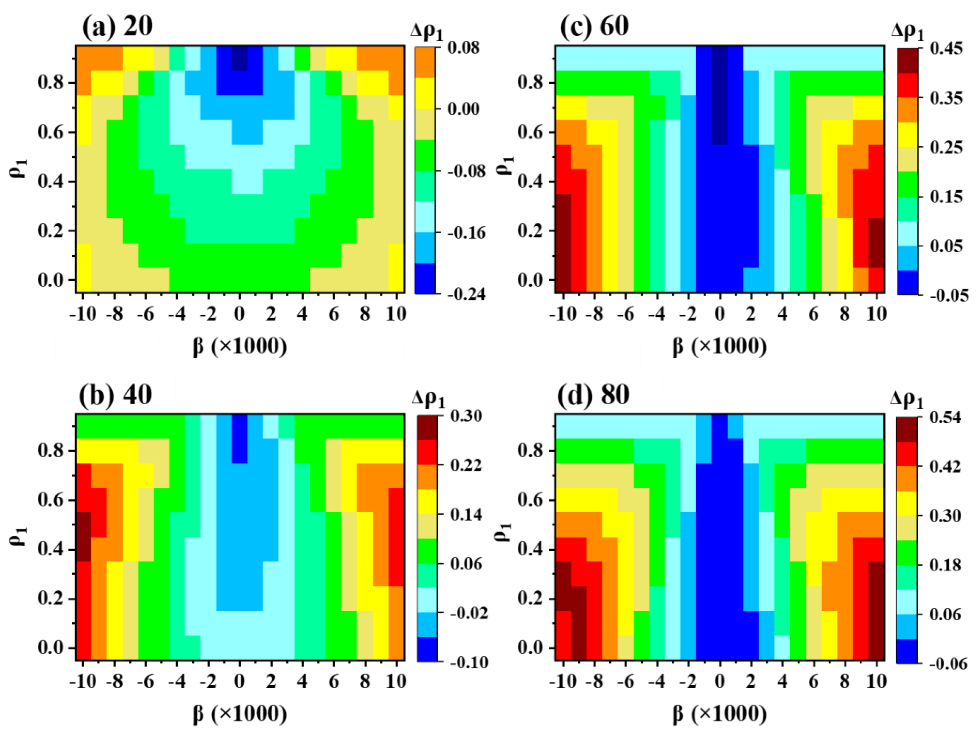
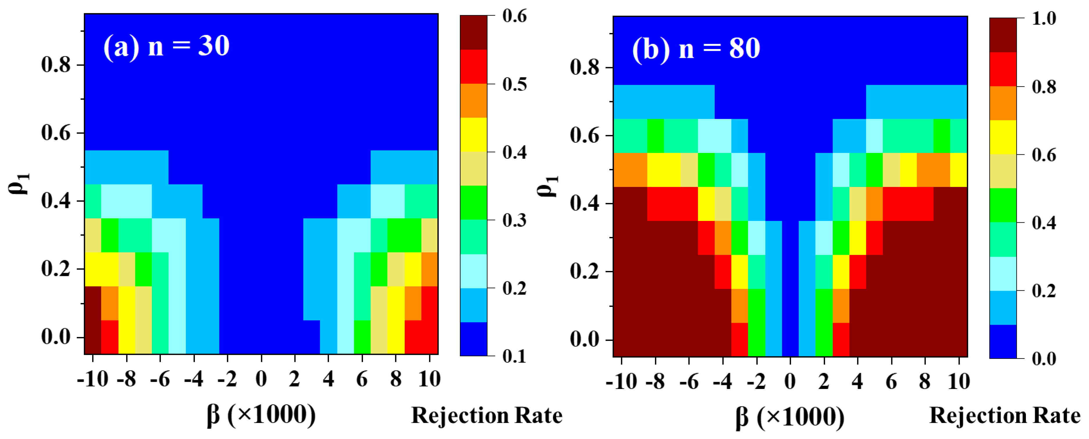
Figure 1 demonstrates the relationship between the trend and the lag-1 autocorrelation (∆ρ₁ = ρ_T − ρ₁; where ρ_T represents the lag-1 autocorrelation after incorporating the trend in the AR(1) series). The findings indicate that weak trends (less than 0.003) have a minimal impact on ρ₁. However, a medium-to-strong trend exhibits a notable impact on ρ₁. The significance of this effect varies depending on the sample size, with a more pronounced impact observed in larger series.

For small samples, the effect of a strong trend on ρ₁ is not particularly significant. However, as the series size increases, the influence becomes considerably more prominent. In the case of medium ρ1 values (ranging from 0.3 to 0.6), a strong trend (β > 0.006) leads to an almost twofold increase in the lag-1 autocorrelation. Furthermore, for low ρ₁ values (ranging from 0.0 to 0.3), the inclusion of a strong trend results in ρ₁ shifting to the upper medium range (0.4 to 0.6).

It is worth noting that when examining detrended data that already exhibited a high level of correlation (greater than 0.8), the resulting ρ_T values were very high (>0.95). The instances where ρ₁ = 0.9 and ρ_T surpassed 0.98 for medium to high trends highlight a potential challenge for trend analysis using the Mann–Kendall (MK) statistic, even after prewhitening the time series.

Figure 1 highlights the sensitivity and complexity of the lag-1 autocorrelation to both the magnitude of the trend and the length of the time series, and derive a definitive empirical formula to precisely remove the effect of autocorrelation in such cases is very challenging.

3.2. Performance of Prewhitening Schemes

3.2.1. Slope Estimation

Figure 2 presents the Sen’s slope estimated using different prewhitening (PW) methods. It is observed that at weak trends, none of the mentioned time series is able to accurately reproduce the actual slope value. Instead, they tend to overestimate the trend, especially when the sample size is small. This overestimation is a result of errors introduced by the series due to the combination of small trends (β = 0.002) and limited sample size (n = 30).

As the actual trend of the series increases, the performance of all PW methods improves as the rejection rate increases. For series with moderate to high trends and a sufficient sample length (β ≥ 0.006 and n ≥ 60), the slopes estimated from the original (ORG), VCTFPW, and DPWMT series are close (within a ±20% range) to the actual trend. However, PW-S struggles to maintain the actual trend when confronted with high serial autocorrelation, resulting in a significant underestimation of the slope due to the loss of prominent trends during the ρ₁ removal process.

PW-Cor preserves the trend of the original series until ρ₁ > 0.5, after which it begins to deviate as the serial correlation increases. TFPW-WS follows a similar pattern to PW-Cor but exhibits extraordinary divergence at ρ₁ ≥ 0.7. To maintain the figure scale, this pronounced deviation is depicted separately (see Figure 3).

Figure 3 showcases the RMSE calculated from the TFPW-WS slope estimator. The RMSE remains relatively low for TFPW-WS when the lag-1 autocorrelation is low (ρ₁ > 0.5). However, the error escalates exponentially as ρ₁ increases. This divergence in slope estimation is particularly pronounced in series with limited sample sizes, potentially stemming from the iterative process of TFPW-WS on highly correlated data. Consequently, a sufficiently large sample size is necessary to mitigate this issue.

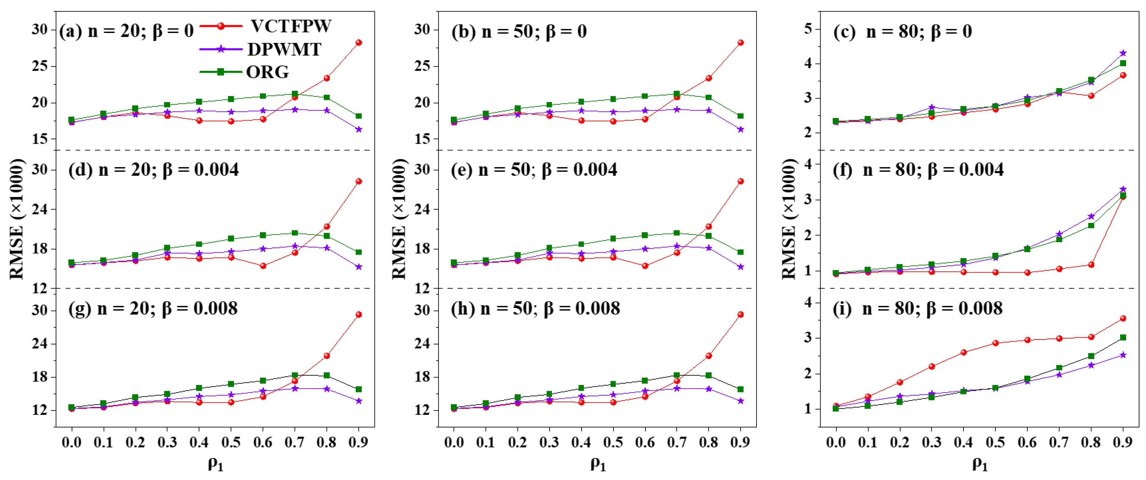
Figure 4 compares the root-mean-square error (RMSE) of the three slope estimators: original series (ORG), VCTFPW, and DPWMT. The results show that VCTFPW performs better than both ORG and DPWMT when the series has moderate lag-1 autocorrelation (ρ₁ between 0.3 and 0.6). However, VCTFPW’s RMSE increases significantly when ρ₁ exceeds 0.6. Conversely, the DPWMT exhibits stable performance across varying levels of ρ₁ and often has a lower RMSE compared to ORG. While VCTFPW yields lower RMSE than DPWMT for mid-range values of lag-1 autocorrelation, the difference is not large enough to outweigh the fluctuations observed in the slope estimation of VCTFPW at mid-high ρ₁.

These fluctuations indicate the underestimation of the slope as ρ₁ increases (as shown in Figure 2). In addition, it is also noted that the length of the series significantly influences RMSE, with longer time series exhibiting notably lower RMSE compared to shorter ones. This indicates an enhanced accuracy in both the estimated slope (β′) and the actual slope (β) for time series with a large sample size. Overall, the DPWMT time series should be used to estimate the trend of a series to obtain an unbiased slope estimation.

3.2.2. Type-I Error

Figure 5 presents the performance evaluation of different PWs in terms of their ability to reject the null hypothesis that assumes the presence of a statistically significant trend. Among the evaluated methods, all series except the original (ORG) and TFPW-Y demonstrate satisfactory results. However, the ORG and TFPW-Y series are more likely to reject the null hypothesis, leading to false positive results. Both the ORG and TFPW-Y series are particularly sensitive to serial correlation, and their Type-I error rates increase significantly as the lag-1 autocorrelation coefficient rises. This means that these series are more prone to incorrectly detecting a trend when none exists due to the influence of autocorrelation.

PW-S and VCTFPW exhibit Type-I error rates that remain consistently below the significance level (α = 0.05). However, the other prewhitening methods, such as PW-Cor, TFPW-WS, and DPWMT, have Type-I error rates slightly higher than the predetermined significance level for the smaller sample sizes. However, as the sample size increases, the Type-I error rates converge to an acceptable level, suggesting improved performance and better control over false positives with larger datasets.

3.2.3. Power of the Test

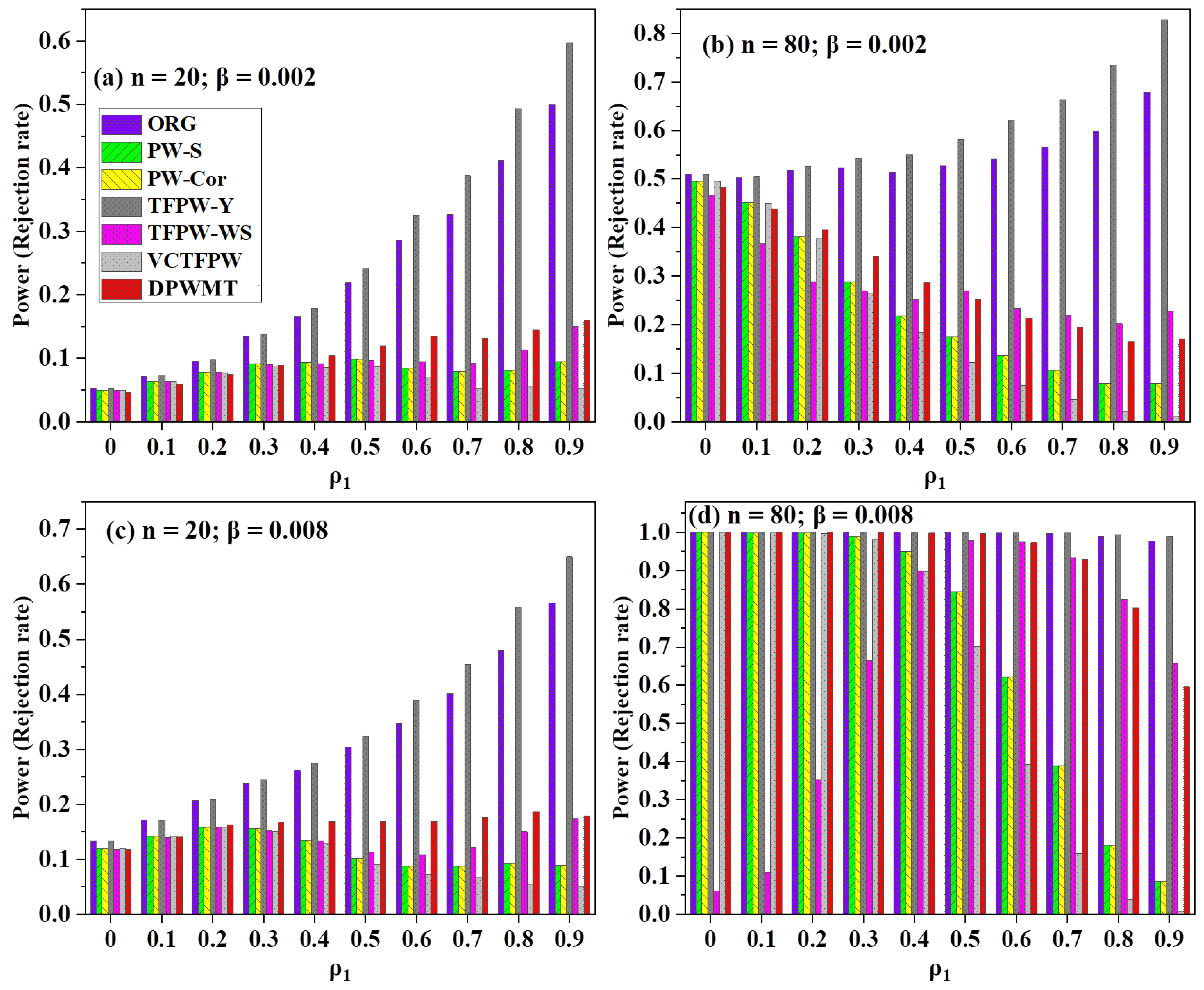
The statistical powers of different prewhitening (PW) methods in detecting significant trends were assessed (Figure 6). The results show that the methods varied in their ability to detect trends. The original series (ORG) and TFPW-Y exhibit moderate power at low sample sizes, but their power exhibits considerable fluctuations as the lag-1 autocorrelation (ρ₁) increases, particularly demonstrating reduced power for weak autocorrelated series. Conversely, the remaining PW methods fail to provide sufficient power for weak trend slopes and short time series.

As the sample size increases, all PW methods exhibit a notable improvement in power for weak serial autocorrelation (ρ₁) but experience a subsequent decrease in power as ρ₁ continues to rise. Notably, the DPWMT and TFPW-WS methods demonstrate relatively higher power retention as the serial correlation increases compared to PW-S, PW-Cor, and VCTFPW. However, for strong trends and longer time series, PW-S, PW-Cor, and VCTFPW struggle to sustain power as ρ₁ increases, with power levels dropping to less than 40% at ρ₁ ≥ 0.7. In contrast, the new method remains suboptimal but maintains approximately 80% power at ρ₁ = 0.8 and around 60% power at ρ₁ = 0.9, enabling the detection of the most significant trends.

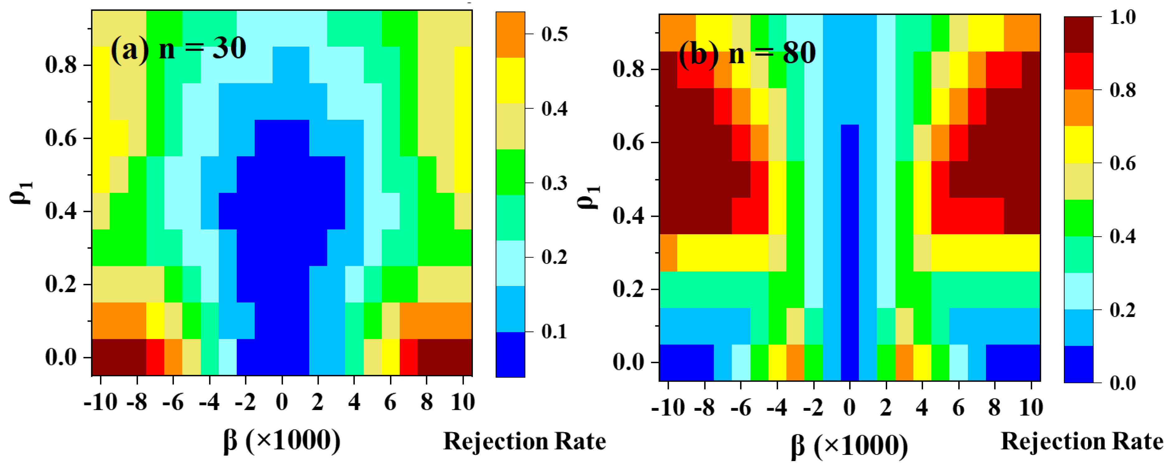
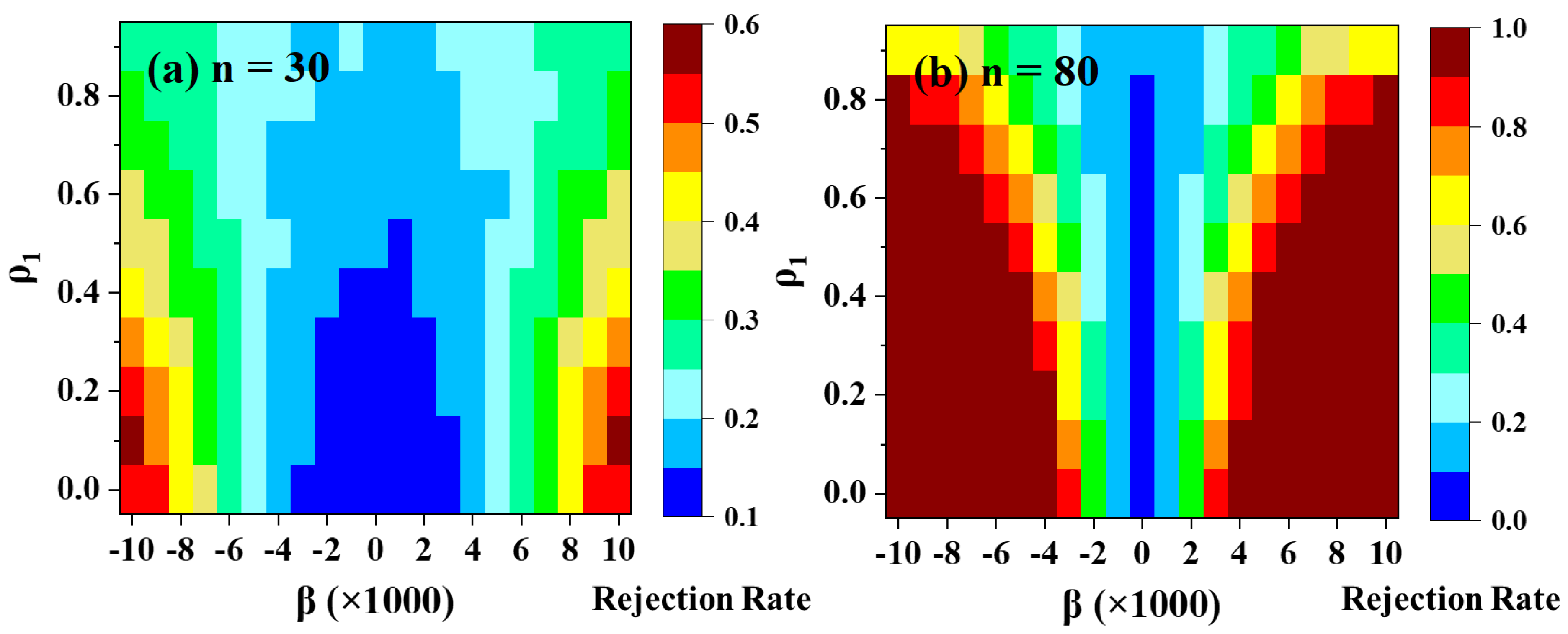
A detailed analysis of TFPW-WS, VCTFPW, and the new method is presented in Figure 7, Figure 8 and Figure 9, focusing on their performance relative to lag-1 autocorrelation, trend size, and the length of the series. For short time series (n = 30), TFPW-WS and DPWMT exhibit limited power for low trends (β = ±0.001 to ±0.004), gradually improving to moderate power for medium to strong trends (β = ±0.004 to ±0.01). In contrast, VCTFPW demonstrates weak power across the entire range of trends, except for scenarios involving weak lag-1 autocorrelation combined with strong trends.

The behavior of the aforementioned methods in longer time series (n = 80) presents intriguing findings. TFPW-WS displays strong power for medium to high serial correlation (ρ₁ > 0.5) in the presence of strong trends yet struggles to maintain power for weak ρ1. Conversely, VCTFPW exhibits a reversed pattern, with higher power observed at low ρ₁, gradually diminishing to moderate levels as ρ₁ increases. The increased test power of TFPW-WS at ρ₁ > 0.5 can be attributed to its divergent behavior at high ρ₁, resulting in elevated slope values, as previously discussed. On the other hand, VCTFPW’s failure to restore power at high ρ₁ may stem from its tendency to underestimate trend magnitudes for highly autocorrelated samples.

Ultimately, the new method proves superior, consistently maintaining the highest power across the entire range of ρ₁ for medium to high trends, making it the recommended approach for unbiased slope estimation and accurate trend detection.

3.3. Case Study

The new PW scheme, along with other PWs, is tested for the particle size distribution and black carbon mass concentration over Mukteshwar (MUK) (29.47° N, 79.6° S; 2.18 km above mean sea level) in India. Further, we analyzed the size distribution data measured at the Pallas-Sodankylä Global Atmosphere Watch (GAW) Station (67.97° N, 24.12° S; 0.56 km above mean sea level) in northern Finland in the subarctic region. The particle size distribution was measured using a differential mobility particle sizer (DMPS assembled by the Finnish Meteorological Institute). The particle number concentrations were calculated in three size bins: nucleation mode N_Nuc (7 to 25 nm particles), Aitken mode N_Ait (25 to 90 nm particles), and accumulation mode N_Acc (90 to 800 nm particles). The black carbon (BC) concentration was calculated using a seven-wavelength aethalometer (Magee Scientific AE-31). The details of the instrument and measurement are available in the previous publications [18].

To address the seasonality in the data, the seasonal MK test [19] is utilized for four seasons: winter (December–February); spring (March–May); summer (June–August); and Autumn (September–November). The annual trends were calculated from the average of seasonal trends and considered statically significant (SS) only if the trends of all seasons were homogeneous at a 90% confidence level and SS at a 95% confidence level [14].

Table 1. Comparison of MK trend results from different prewhitening schemes. ρ_ORG is the lag−1 autocorrelation of the original time series. The statistically significant trends are given in bold.

Parameter (Station) [Year]	Season	ρORG	Slope in %/Year (Z Statistic)
			ORG	PW-S	PW-Cor	TFPW-Y	TFPW-WS	VCTFPW	DPWMT
NNuc (FIN) [2005–2020]	Winter	0.33	0.81 (2.02)	0.63 (0.98)	0.94 (0.98)	0.90 (2.28)	0.91 (1.54)	0.67 (1.53)	0.57 (1.60)
	Spring	0.18	−2.04 (−3.64)	−1.07 (−1.93)	−1.96 (−1.93)	−2.04 (−5.34)	−1.94 (−2.84)	−1.20 (−2.46)	−1.34 (−2.77)
	Summer	0.29	−3.12 (−3.85)	−1.44 (−2.01)	−2.78 (−2.01)	−2.71 (−6.71)	−2.71 (−3.55)	−1.66 (−2.9)	−1.61 (−3.48)
	Autumn	0.28	−1.96 (−1.54)	−0.98 (−1.48)	−1.89 (−1.48)	−1.86 (−4.92)	−1.88 (−2.62)	−1.14 (−2.29)	−1.11 (−2.56)
	Annual		−1.95	−0.71	−1.42	−1.43	−1.41	−0.83	−0.87
NAit (FIN) [2005–2020]	Winter	0.45	2.14 (5.66)	1.13 (2.03)	1.59 (2.03)	1.57 (3.87)	1.61 (2.84)	1.18 (2.69)	1.14 (2.78)
	Spring	0.29	−0.48 (−3.14)	−0.39 (−0.88)	−0.47 (−0.88)	−0.47 (−3.24)	−0.46 (−1.01)	−0.40 (−1.02)	−0.40 (−1.03)
	Summer	0.17	−1.03 (−2.54)	−0.94 (−1.47)	−1.28 (−1.47)	−1.25 (−2.83)	−1.24 (−2.05)	−0.98 (−2.01)	−0.91 (−2.10)
	Autumn	0.37	−0.18 (−2.05)	−0.11 (−0.29)	−0.14 (−0.29)	−0.15 (−2.37)	−0.12 (−0.20)	−0.11 (−0.23)	−0.16 (−0.25)
	Annual		0.11	−0.08	−0.08	−0.08	−0.06	−0.08	−0.08
NAcc (FIN) [2005–2020]	Winter	0.48	1.97 (3.52)	1.37 (2.53)	1.67 (2.53)	1.66 (3.78)	1.64 (3.10)	1.41 (3.09)	1.35 (3.11)
	Spring	0.35	−1.19 (−3.08)	−0.87 (−1.76)	−1.23 (−1.76)	−1.17 (−3.29)	−1.23 (−2.58)	−0.92 (−2.46)	−0.76 (−2.57)
	Summer	0.27	−2.62 (−2.81)	−1.68 (−3.51)	−2.57 (−3.51)	−2.58 (−6.83)	−2.53 (−4.64)	−1.80 (−4.07)	−1.85 (−4.58)
	Autumn	0.37	−1.15 (−2.38)	−0.60 (−1.73)	−0.80 (−1.73)	−0.79 (−2.68)	−0.80 (−2.16)	−0.63 (−2.08)	−0.60 (−2.16)
	Annual		−0.74	−0.44	−0.73	−0.72	−0.73	−0.48	−0.46
NTot (FIN) [2005–2020]	Winter	0.48	0.84 (1.76)	0.43 (0.88)	0.60 (0.88)	0.56 (1.60)	0.61 (1.31)	0.45 (1.23)	0.36 (1.28)
	Spring	0.25	−1.57 (−2.60)	−1.11 (−1.63)	−1.74 (−1.63)	−1.76 (−4.27)	−1.73 (−2.5)	−1.19 (−2.24)	−1.24 (−2.47)
	Summer	0.20	−2.19 (−2.49)	−1.43 (−3.43)	−2.29 (−3.43)	−2.46 (−7.44)	−2.32 (−4.35)	−1.53 (−3.67)	−1.88 (−4.21)
	Autumn	0.39	−1.55 (−3.73)	−0.82 (−1.35)	−1.34 (−1.35)	−1.41 (−3.61)	−1.33 (−1.9)	−0.88 (−1.61)	−1.04 (−1.88)
	Annual		−1.12	−0.73	−1.19	−1.27	−1.19	−0.79	−0.95
NAit (MUK) [2005–2013]	Winter	0.56	4.64 (5.25)	2.12 (2.85)	4.86 (2.85)	4.76 (6.19)	4.85 (2.96)	2.69 (2.37)	2.52 (3.15)
	Spring	0.42	5.00 (5.85)	3.12 (3.79)	5.37 (3.79)	5.21 (6.23)	5.34 (4.05)	3.64 (3.51)	3.37 (3.43)
	Summer	0.58	2.19 (4.54)	1.18 (2.77)	2.83 (2.77)	2.45 (5.10)	2.81 (2.82)	1.55 (2.47)	1.14 (2.94)
	Autumn	0.41	0.62 (0.18)	0.21 (−0.32)	0.35 (−0.32)	0.46 (0.12)	0.35 (−0.32)	0.21 (−0.37)	0.4 (−0.27)
	Annual		3.11	1.66	3.35	3.22	3.34	2.02	1.86
NAcc (MUK) [2005–2013]	Winter	0.48	3.96 (3.78)	2.47 (2.59)	4.76 (2.59)	4.37 (4.47)	4.73 (2.62)	2.91 (2.30)	2.37 (3.35)
	Spring	0.34	4.92 (4.62)	1.51 (1.25)	2.3 (1.25)	3.22 (2.90)	2.4 (1.37)	1.46 (0.94)	3.54 (2.12)
	Summer	0.60	1.52 (2.73)	1.04 (1.95)	2.59 (1.95)	1.95 (3.22)	2.58 (1.96)	1.44 (1.77)	0.76 (1.90)
	Autumn	0.41	−0.05 (−0.68)	−0.27 (−0.84)	−0.45 (−0.84)	−0.29 (−0.87)	−0.45 (−0.84)	−0.32 (−0.84)	−0.03 (−0.51)
	Annual		2.59	1.19	2.3	2.31	2.32	1.37	1.66
BC (MUK) [2005–2016]	Winter	0.34	2.18 (3.63)	1.74 (3.05)	2.65 (3.05)	2.48 (4.33)	2.62 (3.1)	1.89 (2.94)	1.74 (2.84)
	Spring	0.27	2.58 (3.57)	2.33 (3.41)	3.20 (3.41)	3.03 (4.4)	3.18 (3.47)	2.48 (3.31)	2.29 (3.13)
	Summer	0.53	1.40 (2.19)	1.05 (2.09)	2.25 (2.09)	1.58 (2.94)	2.22 (2.11)	1.34 (2.00)	1.16 (2.20)
	Autumn	0.38	1.71 (2.26)	1.48 (2.27)	2.37 (2.27)	2.08 (3.28)	2.36 (2.28)	1.63 (2.15)	1.68 (2.11)
	Annual		1.97	1.65	2.62	2.29	2.60	1.84	1.72

summarizes the results of the MK test performed using various prewhitening (PW) techniques. PW-Cor effectively preserves the underlying trend of the original series. TFPW-Y and TFPW-WS exhibit similar patterns to PW-Cor, mainly because the lag-1 autocorrelation is weak in the original time series, as explained in Section 3.2.1. It is important to note that the low-to-lower-medium lag-1 autocorrelation (ρ1) estimated from the original time series, as presented in Table 1, does not accurately represent the true serial autocorrelation due to the presence of a trend component in the series, as discussed in detail in Section 3.1. Therefore, the actual ρ1 values are expected to be considerably lower than the estimates. Furthermore, TFPW-WS may produce unrealistically high estimates for the slope when dealing with datasets containing high serial correlation, as illustrated in Figure 3. The results in Table 1 suggest that the VCTFPW and DPWMT tests yield a lower-moderate slope estimator of the trend, which is overestimated and underestimated by the ORG and PW-S tests, respectively. This pattern aligns with findings reported by Wang et al. [11].

The Z-statistic, an indicator of both Type-I and Type-II errors (test power), has been calculated to assess the performance of the PW schemes. The TFPW-Y yields the largest absolute value of Z followed by the ORG series and thus indicates the highest Type-I error. However, Type-I errors and the power of the test are complementary to each other; therefore, it may be argued that the time series actually consists of an SS trend and that TFPW-Y and ORG have higher test power than high Type-I errors. However, this rationale does not apply when the number of samples used for the MK test is sufficiently large and the ρ₁ is low to medium, resulting in similar powers of the test as found in VCTFPW and DPWMT (See Figure 6b,d).

The results demonstrate that PW-S exhibits the lowest |Z| values, followed by VCTFPW and DPWMT. It is noteworthy that TFPW-WS yields comparable |Z| values to VCTFPW and DPWMT despite the initially weak autocorrelation. This unexpected outcome can be attributed to the utilization of a large sample size (exceeding 500 in the present cases). Large sample sizes have the effect of inflating |Z| values and significantly enhancing the test power [4]. The DPWMT results match those of the VCTFPW in terms of the trend and the |Z| value, and they support the outcomes derived from the Monte Carlo simulation. Furthermore, the low RMSE value associated with the DPWMT slope estimator, in comparison to VCTFPW, suggests the DPWMT method for unbiased slope estimation.

3.4. Discussion

The prewhitening methods discussed here focus solely on lag-1 autocorrelation. However, atmospheric processes might sometimes be more accurately represented by higher-order autoregressive models that incorporate partial correlations at lags greater than 1 [4]. While considering that these higher-order lag correlations could potentially enhance prewhitening by incorporating the appropriate number of lags, this approach was not examined in this study. Klaus et al. [20] utilized higher-order autoregressive prewhitening for stable oxygen and hydrogen isotopes in precipitation and found that while higher-order lags significantly reduced the variance of the series, the trend slope was relatively unaffected. Moreover, Hardison et al. [21] demonstrated through Monte Carlo simulations involving 124 ecosystem time series that AR(2) autocorrelation (with a coefficient of 0.2) produced similar Type-I and -II error rates for the Mann–Kendall (MK) test and the TFPW-Y as strong AR(1) autocorrelation.

Time series with noticeable seasonality may also show seasonality in lag-1 autocorrelation. Attempts were made to compute lag-1 autocorrelation for various temporal segments rather than the entire series. However, this approach was not pursued further due to the challenges in applying seasonal lag-1 autocorrelation consistently, which resulted in erratic outcomes and precluded the application of the prewhitening method uniformly across all temporal segments.

These prewhitening methods rely on the assumption of linear trends within the time series but do not account for the sensitivity of power to the shape of these trends. Despite this, the linear trend tests offer a reference point for assessing the significance of monotonic nonlinear trends and provide insight into the magnitude of change [11].

The AR(1) model is recognized for its capacity to maintain essential statistical characteristics of hydrometeorological time series, including serial mean, variance, and autocorrelation [22]. However, some research has employed the PW approach with different autocorrelation models, such as the Auto-Regressive Moving Average (ARMA(1,1)). In such cases, more generalized formulas for calculating Variance Inflation Factors (VIFs) that accommodate various autocorrelation structures can be referred to as those proposed by Matalas and Sankarasubramanian [12].

4. Conclusions

This study evaluated the performance of various prewhitening (PW) approaches, including the newly proposed PW method, in estimating linear trends and detecting their significance in the presence of serial autocorrelation. The key findings of the study are the following:

• The magnitude of the trend and length of the time series substantially influence the lag-1 autocorrelation. Strong positive trends result in a noticeable increase in autocorrelation, with a more pronounced impact observed in the series with the large sample sizes.
• All PW methods tend to overestimate weak trends, especially in smaller sample series. As the actual trend increases, the VCTFPW and DPWMT provide the most accurate slope estimations, staying within 20% of the true value. PW-S underestimates the slope considerably due to removing a significant portion of the trend along with ρ₁ removal.
• VCTFPW demonstrates marginally lower RMSE compared to the ORG and DPWMT for mid-range autocorrelation values but fluctuates at higher ρ₁, resulting in slope underestimation. DPWMT exhibits stable RMSE across all ρ₁ values, emerging as the optimal approach for unbiased slope estimation.
• The ORG and TFPW-Y fail to control the Type-I error rate, exhibiting inflated false positive rates with increasing autocorrelation. PW-S and VCTFPW maintain Type-I errors below the significance level across all ρ₁. The remaining methods demonstrate acceptable Type-I error control for larger sample sizes. All PW techniques except TFPW-Y provide insufficient power for weak trends and small samples.
• As the time series length grows, DPWMT and TFPW-WS retain the highest power as autocorrelation strengthens. However, PW-S, PW-Cor, and VCTFPW experience a considerable decline in the power of the test at high ρ₁. TFPW-WS shows high power of the test, but only for high ρ₁ combined with strong trends. In contrast, VCTFPW struggles to restore power at increasing ρ₁ due to slope underestimation. DPWMT maintains the high power of the test across all ρ₁ levels for medium to strong trends.
• In summary, the proposed new PW approach demonstrates clear advantages over existing PW methods. It provides unbiased slope estimation, preserves reasonable control over Type-I error, and maintains sufficient power of the test for detecting trends in the presence of a serial correlation.