Article

Comprehensive Air Quality Model with Extensions: Formulation and Evaluation for Ozone and Particulate Matter over the US

by
Christopher Emery
1,*,
Kirk Baker
2,
Gary Wilson
1 and
Greg Yarwood
1
1
Ramboll, Novato, CA 94945, USA
2
US Environmental Protection Agency, Research Triangle Park, NC 27711, USA
*
Author to whom correspondence should be addressed.
Atmosphere 2024, 15(10), 1158; https://doi.org/10.3390/atmos15101158
Submission received: 14 August 2024 / Revised: 24 September 2024 / Accepted: 24 September 2024 / Published: 27 September 2024
(This article belongs to the Section Air Quality)

Abstract

:
The Comprehensive Air Quality Model with extensions (CAMx) is an open-source, state-of-the-science photochemical grid model that addresses tropospheric air pollution (ozone, particulates, air toxics) over spatial scales ranging from neighborhoods to continents. CAMx has been in continuous development for over 25 years and has been used by numerous entities ranging from government to industry to academia to support regulatory actions and scientific research addressing a variety of air quality issues. Here, we describe the technical formulation of CAMx v7.20, publicly released in May 2022. To illustrate an example of regional and seasonal model performance for predicted ozone and fine particulate matter (PM2.5), we summarize a model evaluation from a recent 2016 national-scale CAMx application over nine climate zones contained within the conterminous US. We show that statistical performance for warm season maximum 8 h ozone is consistently within benchmark statistical criteria for bias, gross error, and correlation over all climate zones, and often near statistical goals. Statistical performance for 24 h PM2.5 and constituents fluctuate around statistical criteria with more seasonal and regional variability that can be attributed to different sources of uncertainty among PM2.5 species (e.g., weather influences, chemical treatments and interactions, emissions uncertainty, and ammonia treatments). We close with a mention of new features and capabilities that are planned for the next public releases of the model in 2024 and beyond.

1. Introduction

Photochemical grid models (PGMs) simultaneously predict concentrations for numerous primary and secondarily formed air pollutants according to a set of chemically coupled, deterministic (prognostic), Eulerian mass conservation equations [1]. The equations are discretized in time over a series of timesteps and in space on a fixed array of three-dimensional grids. By numerically integrating the equations forward in time, PGMs simulate the spatial evolution of pollutant emissions, chemical interaction, transport, and removal. This technique is especially suitable to address complex non-linear chemical interactions among multiple compounds, which is necessary to address the formation and fate of ozone, secondary particulate matter (PM) and toxic compounds that derive from emitted precursors. PGMs are valuable tools with which to evaluate pollutant impacts on public health and natural ecosystems, and to identify efficient paths toward air quality goals.
The Comprehensive Air Quality Model with extensions (CAMx) is an open-source (www.camx.com, accessed on 14 August 2024), state-of-the-science PGM that addresses tropospheric air pollution (ozone, particulates, air toxics) over spatial scales ranging from neighborhoods to continents. Numerous government agencies and consortiums, academic and research institutions, and stakeholders around the world have sponsored CAMx developments and have applied CAMx to support regulatory assessments and scientific research addressing a variety of air quality issues [2,3,4,5,6,7]. The US Environmental Protection Agency (EPA) and many US state and local air agencies rely on CAMx to develop and evaluate emission reduction rules and air quality management plans that address attaining the National Ambient Air Quality Standards (NAAQS) for ozone and PM [8,9,10,11] as well as regional visibility conditions and projected trends [12]. In numerous multi-model comparison studies over the years (e.g., [13,14,15,16]), CAMx generates consistent results with other widely used PGMs around the world while sharing similar sources of uncertainty.
CAMx model design features include:
  • Flexible domain definitions with two-way grid nesting on a variety of Cartesian map projections or geodetic (latitude/longitude) coordinates;
  • Multiple gas phase chemistry mechanism options;
  • Multiple comprehensive inorganic and organic aerosol chemistry treatments;
  • Probing Tools including source apportionment, sensitivity analysis, process analysis, and adjunct reactive tracer chemistry to address specific user-defined air toxics;
  • A sub-grid convective cloud mixing module;
  • Surface bi-directional ammonia exchange;
  • A surface heterogenous chemistry/reemission model;
  • Shared and distributed memory parallelization.
CAMx comprises the core component of an integrated air quality modeling system (Figure 1). As a stand-alone “off-line” model, inputs of space- and time-resolved meteorology, emissions, surface topology, and initial/boundary conditions are developed using independent third-party models and processing tools. Interface programs are needed to translate the products from each of these sources into the specific input fields and formats required by CAMx. After an air quality simulation is completed, additional post-processing programs manipulate raw concentration and deposition output fields for evaluation, visualization, and regulatory analyses.
In this paper we describe the core functionality of CAMx v7.20 (Section 2), which was publicly released in May 2022 [17]. While v7.20 includes miscellaneous minor improvements and features since the release of v7.00 in 2020, these updates have not fundamentally altered the operation or performance of the core model in the v7 series. The description of CAMx v7.20 herein establishes a foundational narrative as the basis for several forthcoming important chemistry and other updates currently being developed for public releases in 2024–2025, which will be described and evaluated in future publications. Section 3 summarizes a model evaluation for ozone and fine particulate matter (PM2.5) for a recent annual application over the conterminous US conducted by the EPA. Section 4 closes with a mention of forthcoming model developments and improvements that will be addressed in future publications. For brevity, the Probing Tool options are not addressed here, but are fully described in the CAMx User’s Guide [17]. We refer the interested reader to the User’s Guide for more detailed information on model formulation, input/output requirements, Probing Tools, and guidance on model installation, configuration and application.

2. Core Model Formulation

The CAMx Reynolds-averaged Eulerian continuity equation predicts the time-rate of change in mass concentration c of species l in Cartesian or geodetic horizontal and terrain-following vertical coordinates. In the Reynolds-averaged formulation, concentrations, meteorological parameters, and rates for emission, deposition, and chemistry are represented as averages over each grid cell and timestep. Higher-order perturbation terms for unresolved turbulent motion are closed (replaced) with a first-order eddy viscosity technique referred to as K-theory. As shown below, the first two terms on the equation’s right-hand-side represent horizontal advection and net vertical exchange across the time/space-undulating absolute vertical coordinate, followed by horizontal diffusion, vertical diffusion, emission injection, wet deposition, and chemistry:
c l t = m 2 A z · A z v c l m η c l z + c l z z t + m · m ρ K c l / ρ + z ρ K z c l / ρ z + m 2 E l x y z Λ l c l + c l t Chemistry   ,
where t is the time coordinate, x, y, and z are spatial coordinates, ∇(x,y) is the horizontal vector differential operator, v(x,y) is the horizontal wind vector, Az(x,y,z) is the cell vertical cross-sectional area, m(x,y) is the ratio of the transformed distance on the Cartesian map projection to true distance (m = 1 for geodetic coordinates), η(x,y,z) is the net vertical transport rate, K(x,y,z) is the horizontal diffusion coefficient, Kz(x,y,z) is the vertical diffusion coefficient, ρ(x,y,z) is atmospheric density, El(x,y,z,l) is the species mass emission rate, and Λ l(x,y,z,l) is the species wet scavenging coefficient. Diffusion coefficients K and Kz are independently determined from input meteorological fields and applied uniformly to all species.
Chemistry comprises mechanism-specific matrices of coupled reaction equations, where many of the reaction rates depend non-linearly on concentration, species properties, and environmental conditions. Pollutant removal includes both dry and wet deposition processes. Dry deposition refers to the direct sedimentation and/or diffusion of material to various terrestrial surfaces and the uptake into vegetation. Dry deposition is treated as a first-order process, where a deposition velocity is calculated for each species and applied as the surface boundary condition for vertical diffusion. Wet deposition refers to the uptake of material into cloud water and precipitation, and its subsequent transfer to the surface. The efficiency with which wet and dry deposition processes can remove pollutants from the air depends upon the physical and chemical properties of the pollutants, local meteorological conditions, and for dry deposition, the type of surface to which they are being deposited.
CAMx internally assigns gridded concentrations and meteorological parameters in an arrangement known as a “C-grid” variable staggering configuration [18]. Scalar variables are located at the cell center representing grid cell averages while wind vector components and diffusion coefficients are carried at cell interfaces to quantify inter-cell mass fluxes. CAMx supports two-way grid nesting, which allows cost-effective applications over large regions with coarser resolution to address regional transport while providing fine resolution nests to address small-scale impacts in selected areas. Two-way nesting allows pollutant concentrations to propagate up- and down-scale among horizontal grid domains of differing resolutions during a single simulation. Any number of grid nests can be specified in a single run, but the vertical grid structures must be consistent among all grids.
Table 1 summarizes the numerical treatments and solvers used for each term of the continuity equation. CAMx employs peer-accepted algorithms and formulations as its technical foundation. The model numerically marches forward in time, applying an operator-splitting approach that calculates the separate contribution of each term to concentration change within each grid cell. A master time step is dynamically determined during the simulation for the largest and coarsest (master) grid based on horizontal winds and grid spacing that ensures a stable explicit advection solution for Courant numbers between 0.5 and 1.0. Timesteps typically range within 5–15 min for grid cell sizes of 10–50 km and can be a minute or less for cell sizes of 1–2 km. Nested grids require multiple timesteps per master step depending on their grid resolution relative to the master grid. Additional sub-steps are used as necessary within individual processes such as chemistry to ensure accurate and stable solutions within each grid cell.

2.1. Emissions

Pollutant emissions are provided as hourly, chemically speciated, gridded and stack-specific (point) input files. Each point source stack is defined by unique spatial coordinates and parameters that determine plume rise. Emission rates are held constant over each input hour rather than interpolated to each timestep. Third-party emission processing systems and models are used to develop emission input files for CAMx. Emissions are specified in units of mol/h (gasses) or g/h (PM). CAMx can read any number of gridded and point emission files stratified by source sector.
Two-dimensional gridded emissions represent numerous widespread sources that emit near the surface, such as vehicles, commercial and residential activities, biogenic and other natural sources. Three-dimensional gridded emissions represent widespread sources that emit aloft, such as aircraft, fires, and lightning NOx. Point sources represent emissions from large industrial stacks. CAMx supports three options to specify stack-specific emission injection heights: (1) externally specifying the final plume centerline height; (2) externally specifying a uniform vertical distribution between plume top and bottom; and (3) internally calculating plume rise based on the multi-layer stability-dependent algorithm of Turner et al. [46] according to stack parameters and time-evolving local ambient meteorological conditions.

2.2. Transport

2.2.1. Advection

CAMx can operate directly on map projections and grid systems employed in widely used prognostic meteorological models so that the translation of meteorological data to CAMx requires as little manipulation as possible. Currently, Ramboll supports a CAMx interface with the Weather Research and Forecasting model (WRF) [47]. The interface processor may (1) pass WRF meteorological data to an identical CAMx grid system, (2) horizontally interpolate WRF data to a different CAMx map projection or resolution, and (3) vertically aggregate data from the WRF layer structure to a coarser structure in CAMx. Gridded meteorological variables are supplied to CAMx at hourly intervals, which are then time-interpolated to individual timesteps.
Three-dimensional advection in CAMx is both mass conservative and mass consistent. Mass conservation refers to the accurate accounting of all sources and sinks of pollutant mass with no spurious loss or gain during model integration. To maintain mass conservation, CAMx solves the transport equations in flux form. Mass consistency refers to the transport of pollutant mass equivalently to the input atmospheric momentum field. Sources of poor mass consistency in any off-line air quality model include the following: (1) supplying meteorology that is inherently inconsistent (e.g., from an interpolative objective analysis or diagnostic model); (2) spatially interpolating or averaging meteorological fields to a different map projection or grid resolution; (3) supplying hourly instantaneous meteorological fields that are subsequently interpolated to the air quality model timesteps; and (4) employing different numerical methods among the meteorological and air quality models. Since each of these factors are always at play to varying degrees, the numerical linkage between the three-dimensional advection components has been developed in a mass consistent fashion to preserve the space/time-evolving input atmospheric density field at each timestep.
Horizontal advection is solved using the Piecewise Parabolic Method (PPM) [19,20], or the non-linear renormalized integrated flux solver of Bott [21]. These finite difference schemes provide higher order accuracy with minimal numerical diffusion yet are equivalent in execution speed compared to other simpler advection algorithms.
CAMx internally calculates an instantaneous vertical velocity field from grid- and timestep-specific horizontal momentum fields to balance the local atmospheric continuity equation, thus ensuring a three-dimensional momentum field that is mass consistent. To calculate a vertical velocity profile w(z), the atmospheric continuity equation is locally integrated through the depth of each grid column with an imposed zero boundary condition at the ground:
ρ w z = 0 z ρ t + m 2 A z · A z v ρ m d z
where the time-rate change in atmospheric density in each grid cell is known from the input meteorological fields. The horizontal flux divergence of atmospheric density is calculated in a manner that is numerically consistent with the procedure used to horizontally advect pollutants, using either the Bott or PPM advection solvers. As a result, a cell- and timestep-specific vertical velocity is constructed that provides a balance between the imposed density tendency, resolved horizontal momentum divergence, and any “apparent” divergences induced by the time/space-undulating vertical coordinate. Further, the net vertical transport rate η(z) is defined as the combination of resolved vertical velocity w(z) and the time-rate of change in the local layer interface height:
η ( z ) = w ( z ) z t
Vertical transport is solved using either PPM or an implicit backward Euler integration scheme developed specifically for CAMx [22].

2.2.2. Diffusion

CAMx employs a first-order eddy viscosity (or “K-theory”) approach to represent diffusive transport by sub-grid turbulence. As a “local” closure technique, K-theory treats mass transfer cell by cell (horizontally) or layer by layer (vertically), analogously to the diffusion of heat through a solid medium.
CAMx internally calculates explicit horizontal diffusion coefficients using a wind deformation approach based on the methods of Smagorinsky [48]. A constant minimum diffusion coefficient is added that varies with horizontal grid spacing consistent with the approach of Anthes and Warner [49]. Horizontal diffusion is solved using an explicit simultaneous two-dimensional flux-divergence calculation.
Like all PGMs, simulated concentration fields are rather sensitive to diurnal variations in the strength and depth of vertical mixing within the planetary boundary layer. For this reason, hourly three-dimensional vertical diffusion coefficients Kz are supplied to CAMx via input files generated by the WRF-CAMx interface or other sources, thereby facilitating Kz sensitivity testing without the need to modify an internal calculation within the CAMx code. The standard K-theory vertical diffusion solver employs an implicit backward Euler integration scheme. Vertical diffusion is solved over potentially several sub-steps, depending upon the magnitude of the vertical diffusivity relative to the vertical layer depths. This technique ensures sufficient diffusive coupling among all layers that exhibits high diffusivity.
An inadequate treatment of deep vertical convective mixing is a known shortcoming of K-theory. In such cases, buoyant plumes deriving energy in the surface layer are quickly and efficiently mixed deep into the atmosphere within eddies that are usually much larger than the individual model layers. This process has been shown to have important ramifications for chemistry, especially during transition periods between stable/neutral and convective conditions [23]. CAMx can optionally be run using the non-local Asymmetric Convective Model (ACM2) [23], which includes (1) mixing among adjacent layers using K-theory; (2) rapid upward non-local mixing from the surface layer to all layers through the boundary layer (the convective aspect); and (3) slower compensating downward mixing layer by layer from the top of the boundary layer to the surface (the asymmetric aspect). CAMx invokes the convective component of the ACM2 during unstable conditions, which is solved separately using a semi-implicit scheme. During non-convective conditions, the ACM2 reverts to local K-theory.

2.3. Dry Deposition

Dry deposition is treated as a first-order removal rate, where the flux of a pollutant to the surface is determined by its “deposition velocity” through the lowest model layer. Deposition velocities are derived from algorithms that account for the reactivity, solubility, and diffusivity of gasses, the size and density of particles, local meteorological conditions, and time-evolving surface characteristics (i.e., seasonal vegetative changes and snow cover). CAMx offers two dry deposition options: one based on Wesely [24] and Slinn and Slinn [26], and the other based on Zhang et al. [25,27]. CAMx determines a set of species-dependent deposition velocities for each land use type present in each grid cell and then linearly combines them according to the fractional land use distribution. The dry deposition flux is used as the lower boundary condition in the vertical diffusion solver. Gasses and PM are assumed to be irreversibly absorbed and/or chemically removed by surface media, so reemission and resuspension effects are ignored.
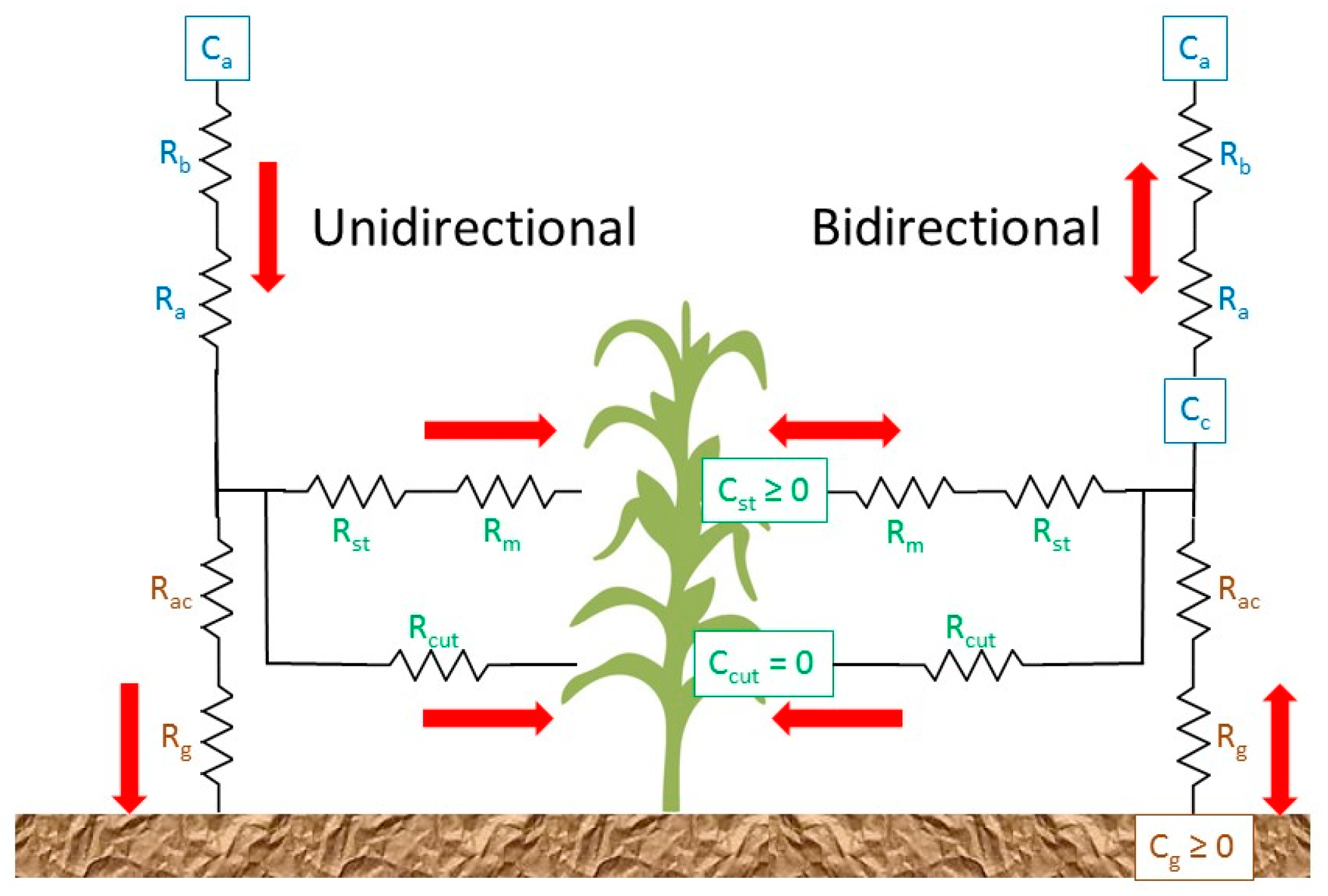
In all cases, the movement of material from the atmosphere through the plant canopy and onto various surface types is modeled analogously to an electric circuit (Figure 2). Resistances in serial and parallel arrangements represent the relative ease with which material moves through different portions of the deposition pathway. In both Wesely and Zhang schemes, for example,
V d = 1 r a + r b + r s
for gasses and
V d = v s e d + 1 r a + r b + r a r b v s e d
for particles. Here, Vd is the deposition velocity, vsed is the particle gravitational settling velocity, and the variable r represents three types of resistances to deposition. Particulate settling depends on size and density, which are affected by the aerosol water content determined from local humidity and PM deliquescence properties according to the PM partitioning models.
An “aerodynamic” resistance ra represents turbulent transport through the lowest model layer, which operates equivalently for all gasses and particles. CAMx employs the surface layer turbulent stress parameterization of Louis [51] for this calculation, which accounts for time- and space-evolving meteorology. A quasi-laminar sublayer or “boundary” resistance rb represents molecular diffusion through the thin layer of air directly in contact with surface elements. It depends on air density and the molecular (gas) or Brownian (PM) diffusivity of each pollutant species.
A set of parallel surface resistances are applied for gas uptake onto various surfaces (leaf stomata, mesophyll and cuticle, upper and lower canopy surfaces, ground soil/debris, and water). The approaches of the Wesely and Zhang schemes differ significantly in this regard. Both build in different baseline sets of surface resistances for SO2 and ozone in their models, and then scale those values to other gas species based on molecular diffusivity, solubility, and reactivity. In both options, CAMx zeros surface resistances for certain acids such as HNO3 given their large and efficient uptake rates to vegetation and other surfaces [52,53]. Over water, the surface resistances in the Wesely scheme for all gas species other than ozone are based on some improvements adopted by Kumar et al. [54] following Sehmel [55]. In both Wesely and Zhang schemes, we modified over-ocean ozone resistances in earlier versions of CAMx to parametrically match the tendencies of measured ozone fluxes reported by Helmig et al. [56] from ship-borne measurements:
r s O 3 = 1 1 × 10 4 + 5 × 10 6   H   T s 3   u *
where H is Henry’s law solubility, Ts is the surface temperature (°C), and u* is the friction velocity. The cubic temperature dependence fits the deposition velocity response to the range of sea surface temperatures reported by Helmig et al. [56].

Bidirectional Ammonia Scheme

The bidirectional ammonia (NH3) algorithm [28] can be optionally invoked when the Zhang deposition scheme is selected. Implemented within the dry deposition function for gasses, the approach assigns NH3 “emission potentials” by terrestrial (non-water) land cover type that determine temperature-dependent “compensation points” (concentrations) along the surface–atmosphere circuit (Figure 2). When compensation points are higher than atmospheric concentrations, the net flux is from the surface to the atmosphere (emission); conversely, the net flux is to the surface (deposition). In all cases with non-zero emission potential, NH3 deposition rates to the surface are reduced (or reversed) relative to the original unidirectional deposition function, the latter of which implicitly assumes zero emission potential.
CAMx assigns the land use-specific emission potentials reported by Whaley et al. [50]. Emission potentials are set to zero if the Leaf Area Index (LAI) is less than 0.5 or if the ground is covered by snow; thus, there is no capacity for emissions from low-vegetation land cover. NH3 emission fluxes calculated from agricultural land use categories are also set to zero on the basis that NH3 emission inventories often explicitly include fertilizer application and thus the bidirectional scheme would potentially double-count NH3 emissions.

2.4. Sub-Grid Convective Cloud Mixing

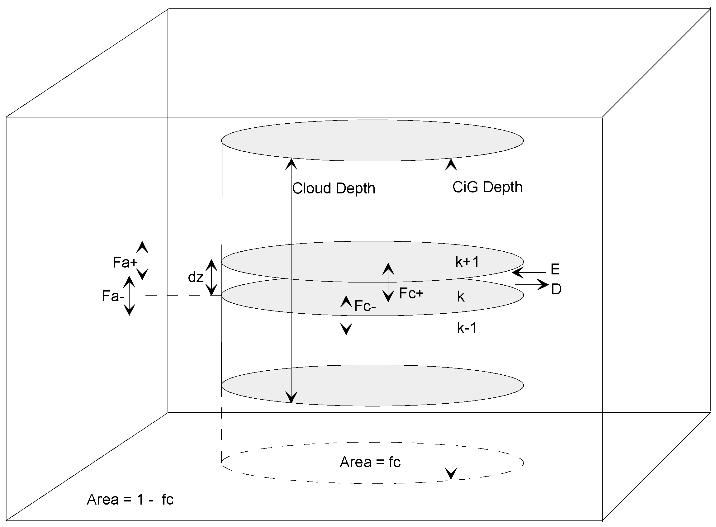
CAMx includes an optional sub-grid cloud framework (Cloud-in-Grid or CiG) that explicitly simulates in-cloud shallow mixing, deep convective transport, aqueous chemistry, and wet scavenging below the grid scale [29]. All processes are driven by output fields generated by the WRF Multi-Scale Kain-Fritsch (MSKF) cumulus parameterization [57,58,59,60,61]. This yields a consistent cloud-mixing-chemistry system across the WRF and CAMx models. Without the CiG invoked, CAMx ignores cloud convective transport and treats all cloud processes at the grid resolution, where diagnosed sub-grid cloud fields are used to parametrically influence grid-scale photolysis rates, wet deposition, and aqueous chemistry.
The CiG defines the physical attributes of a stationary, steady-state, multi-layer sub-grid cloud environment each hour according to cloud and mass flux data provided by WRF/MSKF (Figure 3). Grid-scale pollutant concentration profiles within each grid column are allocated to the CiG and ambient fractions. Vertical transport within the CiG and ambient grid column fractions are coupled in a mass conservative manner according to the vertical integration of horizontal entrainment/detrainment flux profiles and the relative cloud area to ambient column area. The CiG does not distinguish between separate updraft and downdraft fluxes, and instead assumes a well-mixed condition in each layer that allows the use of net vertical fluxes.
The numerical solver for mass transport employs an explicit first-order upstream approach, which needs to take small steps of a few seconds to remain stable and positive-definite. Applying this to thousands of grid columns and hundreds of chemical species at each model timestep would thus severely impact model speed. Instead, CiG solves the evolution of a single matrix of unitless air mass tracers for each convective column at each hourly meteorological update time. As the model integrates over successive timesteps, CiG algebraically combines the final tracer matrix with every column’s chemical profile to yield the net effect of convective dynamics at each timestep. Then, CiG performs aqueous chemistry and wet scavenging separately on the in-cloud and ambient concentration profiles according to resolved and sub-grid cloud and precipitation inputs. Finally, the two chemical profiles are linearly combined to yield the net result of cloud/ambient transport, aqueous chemistry, and the wet removal on the given profile. Gas-phase chemistry and PM thermodynamic equilibrium always operate on the single total column chemical profiles as the last step in the operator splitting sequence, after the CiG processes are completed.
Depending on the scale and intensity of MSKF-diagnosed convection, the CiG parameterization can produce minor to substantial changes in vertical pollutant profiles in those grid columns. The CiG generally improves boundary layer simulations of ozone and nitrogen oxides when compared to aircraft-derived profiles [29]. However, comparisons between CiG and measured pollutant profiles are confounded by the fact that cloud fields are challenging for meteorological models to predict accurately in time and space.
While characterizing steady-state cloud conditions is appropriate for cloud scales approaching grid resolution and hourly time scales, it is an increasingly poor approximation for features at smaller scales. The CiG relies entirely on how sub-grid clouds are derived by the WRF MSKF scheme. The basis for the steady-state assumption stems from the fact that WRF output fields represent an instantaneous “snapshot” of the meteorological variables at each hour. While CAMx interpolates continuous fields of temperature, pressure, and winds across the hour, the model holds discrete cloud fields constant. The CiG approach may therefore alias the actual evolution of sub-hourly cloud fields occurring within WRF. Temporal and spatial interpolation of cloud water and convective mixing rates across the hour would involve additional complicated, and arguably inappropriate, assumptions without adding substantial value.

2.5. Wet Deposition

CAMx calculates wet scavenging from each layer within a precipitating grid column from the top of the precipitation profile to the surface, as determined by the WRF-CAMx interface. First-order scavenging coefficients are determined differently for gasses and PM based on relationships described by Seinfeld and Pandis [1]. Wet deposition is the predominant removal process for fine particles and can be important for soluble gasses, but it is reversible when the aqueous uptake of certain less soluble gasses reaches solubility limits. The rate at which these processes occur depends on numerous meteorological, physical and chemical factors.
The model includes three types of precipitating hydrometeors (rain, snowflakes, and graupel), each separately represented by a single mean size, mass, and fall speed through the precipitating column. These characteristics are parametrically determined from input surface precipitation rate fields based on the approach of Scott [62], with updates to match data assembled by Seinfeld and Pandis [1]. Mixed-phased hydrometeors do not coexist within a single layer—only liquid or one ice form is present depending on temperature and input precipitation data. The monodisperse hydrometeors fall through and scavenge monodisperse cloud water droplets containing particles and dissolved gasses, and also scavenge monodisperse sub-cloud PM.
Gas scavenging includes two rates: (1) the accretion of cloud droplets containing dissolved gasses into precipitation, and (2) the diffusive uptake of ambient gasses into precipitation, which can occur within or below clouds. CAMx assumes that gas concentrations exist in equilibrium between air and cloud water droplets because equilibrium is usually established on time scales of minutes. Air–water partitioning depends on species’ Henry’s law solubility (including any aqueous dissociation) and cloud water temperature and acidity. Ambient gasses may directly diffuse into rain, while only strong acids may diffuse into ice hydrometeors; rates depend on the hydrometeor’s state of saturation as a function of pH, species diffusivity, and aerodynamic considerations. Gasses may be reversibly scavenged by cloud water collection and diffusion; super-saturated gasses are released back to the atmosphere according to their diffusivity.
PM scavenging also includes two rates: (1) the accretion of cloud droplets containing particles into precipitation, and (2) the impaction of ambient particles into precipitation, which occurs only below clouds. All particles are taken up into cloud water (no particles exist in the interstitial air between cloud droplets) and are irreversibly scavenged by cloud water collection and precipitation impaction. Sub-cloud aerosol collection rates from impaction depend on the aerosol size and density that determine a collection efficiency. Snow presents a complication related to aerodynamic drag, which affects PM collection efficiency. To simplify the calculation for snow, the model calculates a collection efficiency for graupel but sets a lower limit based on the work of Sauter and Wang [63].

2.6. Chemistry

Table 2 lists the gas-phase photochemistry mechanisms available in CAMx v7.20. All mechanisms are linked to aerosol chemistry treatments to provide necessary gas precursors. CAMx includes separate algorithms for aqueous aerosol chemistry, inorganic gas–aerosol partitioning, and organic oxidation and gas–aerosol partitioning. Updated CB mechanisms and other gas-phase chemistry schemes are in active development and testing and will be reported in future publications.

2.6.1. Gas-Phase Photochemistry

Yarwood et al. [30] developed the Carbon Bond version 6 (CB6) photochemical mechanism, extending from earlier versions including Carbon Bond version 4 [64] and Carbon Bond version 2005 [65]. CB6 was evaluated against data from 339 chamber experiments conducted at the University of California at Riverside and the Tennessee Valley Authority. Two revisions of CB6 ensued, each adding new compounds, associated reactions, and updated reaction rates: CB6 Revision 1 (CB6r1) [31] and CB6 Revision 2 (CB6r2) [34]. We refer the reader to the cited references for details on the CB mechanism’s lineage through CB6r2.
CB6r2h is an extension of CB6r2 that adds reactions involving a large set of ocean-borne halogen compounds [32]. Bromine reactions were integrated with previously developed reactions for iodine and chlorine [66] with rate constants based on data from the International Union of Pure and Applied Chemistry (IUPAC).
CB6 Revision 4 (CB6r4) combined CB6r2 with temperature- and pressure-dependent NO2-alkyl nitrate branching originally developed in CB6r3 a condensed set of reactions involving ocean-borne inorganic iodine in lieu of the full halogen mechanism in CB6r2h, and the oxidation of ocean-borne dimethyl sulfide or DMS [35,67,68,69,70]. CB6r4 is supported by an in-line parameterization within CAMx that computes inorganic iodine emission fluxes (I2 and HOI) caused by ozone deposition to seawater [71,72]. CB6r4 also adds the pseudo-heterogeneous hydrolysis of isoprene-derived organic nitrate (INTR). Aerosol uptake of organic nitrate followed by particle-phase hydrolysis to HNO3 formation can be an important pathway for the loss of atmospheric NOx [34,73,74]. CB6r4 assumes the same lifetime (1 h) against particle-phase hydrolysis of INTR as described by Fisher et al. [74]. The partitioning of organic nitrate into its particle phase is modeled using a two-product parameterization based on ambient measurement data during the 2010 CalNex [75]. If PM is not explicitly modeled, CAMx assumes equal partitioning between the gas and particle phases.
CB6 Revision 5 (CB6r5) [33] incorporates updates to chemical reaction data from IUPAC and the National Aeronautics and Space Administration (NASA) [76] for inorganic and simple organic species that play a role in ozone formation. Mechanism updates were prioritized for the following:
  • Reaction parameters that contribute most to uncertainty in ozone predictions as determined by Dunker et al. [77];
  • Reactions of simpler organic compounds (i.e., methane, ethane, propane, ethene, ethyne, formaldehyde, acetaldehyde, acetone, benzene, and toluene) with oxidants (i.e., OH, NO3, ozone);
  • Reactions of NOx, HOx, and Ox.
Overall, 132 reactions rates were reviewed and 46 were updated. The updates were based on recommended values from IUPAC and NASA, which had been revised since being implemented in the original CB6. The updates included the following:
  • Rate constants for thermal reactions, i.e., reactions that occur when atoms and/or molecules collide;
  • Stoichiometric coefficients that define product yields for thermal reactions;
  • Absorption cross-sections and quantum yields for photolysis reactions, i.e., reactions that occur when molecules absorb sunlight and chemical bonds are broken.
The Supplemental Information provides a complete listing of CB6r5 species, reactions, and rate expressions.
CAMx also includes the 2007 update of the SAPRC chemistry mechanism (SAPRC07TC), which includes additional model species compared to prior versions. The additional species explicitly represent certain toxics and reactive organic compounds [33]. SAPRC07TC uses numerical expressions of rate constants that are compatible with the current CAMx chemistry mechanism solver. Chlorine chemistry is not included in the CAMx implementation of SAPRC07TC.

2.6.2. Photolysis Rates

Photolysis rates are needed by gas-phase and aerosol chemistry in CAMx. Photolysis rates are externally derived assuming clear-sky conditions as a function of five parameters: the solar zenith angle, the altitude above ground, the total ozone column, the surface albedo, and the terrain height. The rates are provided to CAMx as a lookup table that spans the range of conditions for each of the five dimensions. The user must develop this lookup table using a CAMx pre-processor that incorporates the Tropospheric Ultraviolet and Visible (TUV) radiative transfer model [78]. The TUV model employs a standard atmosphere density profile for Rayleigh scattering and other absorbers such as oxygen and ozone. A user-supplied daily grid of atmospheric ozone column scales the default vertical ozone profile within the TUV model. A default aerosol profile [79] is combined with typical aerosol optical properties within the TUV model to account for a mean global background haze.
As CAMx runs, the clear-sky lookup rates are interpolated to the specific conditions in each grid cell. They are then adjusted for local cloud cover and local aerosol attenuation. Additionally, solar angle-dependent temperature and pressure adjustments are applied to five key photolysis reactions (NO2, ozone, acetaldehyde, and two formaldehyde reactions). CAMx includes a fast in-line version of the TUV model [80] to calculate photolysis adjustment profiles through each cloudy, aerosol-laden grid column. The in-line model is run twice for each grid column: first for non-cloudy conditions with the same aerosol profile used in the external TUV pre-processor, and then repeated with input cloud fields and simulated aerosols to derive a vertical profile of the cloudy:clear actinic flux ratio. This ratio is then applied as a multiplicative factor to the clear-sky value in each grid cell.
CAMx assigns the UV surface albedo according to the distribution of gridded land use fields provided to the model. Snow-free UV albedos range between 0.04 and 0.10, consistent with satellite data for typical terrestrial and water surfaces [81]. CAMx includes a parametrization of snow albedo that accounts for land use type and gridded inputs of snow depth and snow age based on the approach used in the WRF/NOAH land surface model [82,83,84,85].
Model calculations of photolysis rates are subject to uncertainties in the model formulation and input data. Palancar et al. [86] evaluated TUV using aircraft-based measurements and found that the model can perform well given accurate input data. Clouds are likely to be a large source of uncertainty in photolysis calculations because clouds strongly influence solar radiation and are challenging for meteorological models to predict accurately in time and space. For gas-phase chemistry, a global uncertainty analysis of the CB6r4 chemical mechanism [77] found that uncertainty in the NO2 photolysis rate ranked highest of all 682 mechanism parameters even though NO2 photolysis data, i.e., cross-section and quantum yield, have been extensively studied [76]. For SOA chemistry (Section 2.6.4), uncertainty in the ratio of secondary organic aerosol (SOA) to NO2 photolysis rates (discussed below) is likely the greatest contributor to uncertainty in modeling how photolysis influences the fate of SOA.

2.6.3. Gas-Phase Chemistry Solvers

Gas-phase chemistry requires numerically integrating a matrix of coupled ordinary differential equations (ODEs) representing hundreds of reactions. This process is among the most computationally expensive operations performed in a PGM, and so the computational efficiency of the gas-phase chemistry solver strongly influences the overall speed of any grid model. CAMx includes two chemistry solvers that offer trade-offs between accuracy and efficiency. The double precision version of the Livermore Solver for Ordinary Differential Equations (LSODE) [39,87] is used as a reference method for testing new mechanisms and solver techniques. LSODE is highly accurate and stable for such problems but is generally too slow for routine use in grid model applications.
The chemical workhorse in CAMx is the Euler Backward Iterative (EBI) method as implemented by Hertel et al. [38]. In general, the backward Euler method must be iterated to convergence because species concentrations are interdependent. Like LSODE, the basic EBI method is not efficient for stiff problems such as tropospheric chemistry because convergence is slow, and the step size must be short. Hertel et al. [38] greatly improved the efficiency and accuracy of the method by developing analytical solutions to the EBI equation for groups of species that are strongly coupled (e.g., HOx and NOx/ozone).

2.6.4. Aerosol Chemistry

The CAMx aerosol treatment treats the PM size distribution as two static modes, coarse with aerodynamic mean diameters >2.5 µm, and fine with mean diameters ≤2.5 µm (referred to as “CF”). Directly emitted or “primary” PM species can be modeled as fine and coarse particles, while all chemically formed or “secondary” PM species are modeled as fine particles only. Aerosol chemical processes include the following:
  • Aqueous sulfate and nitrate formation in resolved cloud water is calculated using the RADM-AQ algorithm [43], which includes updated SO2 oxidation reaction rates and metal-catalyzed oxidation [87,88,89,90] and the aqueous formation of SOA from glyoxal, methyl glyoxal and glycolaldehyde [91,92].
  • Inorganic gas-particle partitioning is determined using ISORROPIA v1.7 [40,41] or EQSAM4clim [42]; ISORROPIA addresses sulfate, nitrate, chloride, ammonium, and sodium, with an update for calcium nitrate on dust particles, while EQSAM addresses the same species and includes the additional cations of magnesium and potassium.
  • Organic oxidation chemistry and gas-particle partitioning are determined using an updated two-product equilibrium scheme called SOAP [44] or a hybrid 1.5-dimension volatility basis set (VBS) approach [45].
Inorganic PM includes sulfate, nitrate, ammonium, aerosol water, sodium, chloride, elemental carbon, and general categories representing other primary and crustal (dust) compounds. Eight explicit fine-mode elemental species can be optionally simulated: Fe, Mn, Ca, Mg, K, Al, Si, and Ti. If these are not modeled, then CAMx sets default background values for chemical calculations. Five elements (Fe, Mn, Ca, Mg, and K) are used by the RADM-AQ aqueous chemistry; Fe and Mn catalytically contribute to the oxidation of SO2 to sulfate, while Ca, Mg, and K impact cloud pH and thus the solubility of SO2 in cloud water. Three elements (Mg, Ca, and K) influence inorganic aerosol partitioning in EQSAM, and one (Ca) influences dust nitrate (CaNO3) in ISORROPIA. All eight are used along with other fine primary and crustal components to determine the fine dust surface area for heterogenous reactions of SO2 and N2O5.
The uptake of SO2 and HNO3 by dust particles is a potentially important heterogeneous reaction pathway. The heterogeneous reaction of SO2 with oxidants on the particle surface assumes a pseudo first-order reaction with the humidity-dependent uptake coefficient by Zheng et al. [93]. HNO3 reacts with calcium in soil dust particles to form calcium nitrate. Since the ISORROPIA implementation in CAMx does not consider cations other than sodium, the heterogeneous production of calcium nitrate is treated separately. If calcium is explicitly modeled, its concentration is used directly; if it is not modeled, CAMx assumes a 6% mass fraction of calcium carbonate (CaCO3) in fine dust particles based on Saharan dust study [94], and half of it is assumed to be replaced by calcium nitrate. EQSAM addresses HNO3 interactions with calcium explicitly.
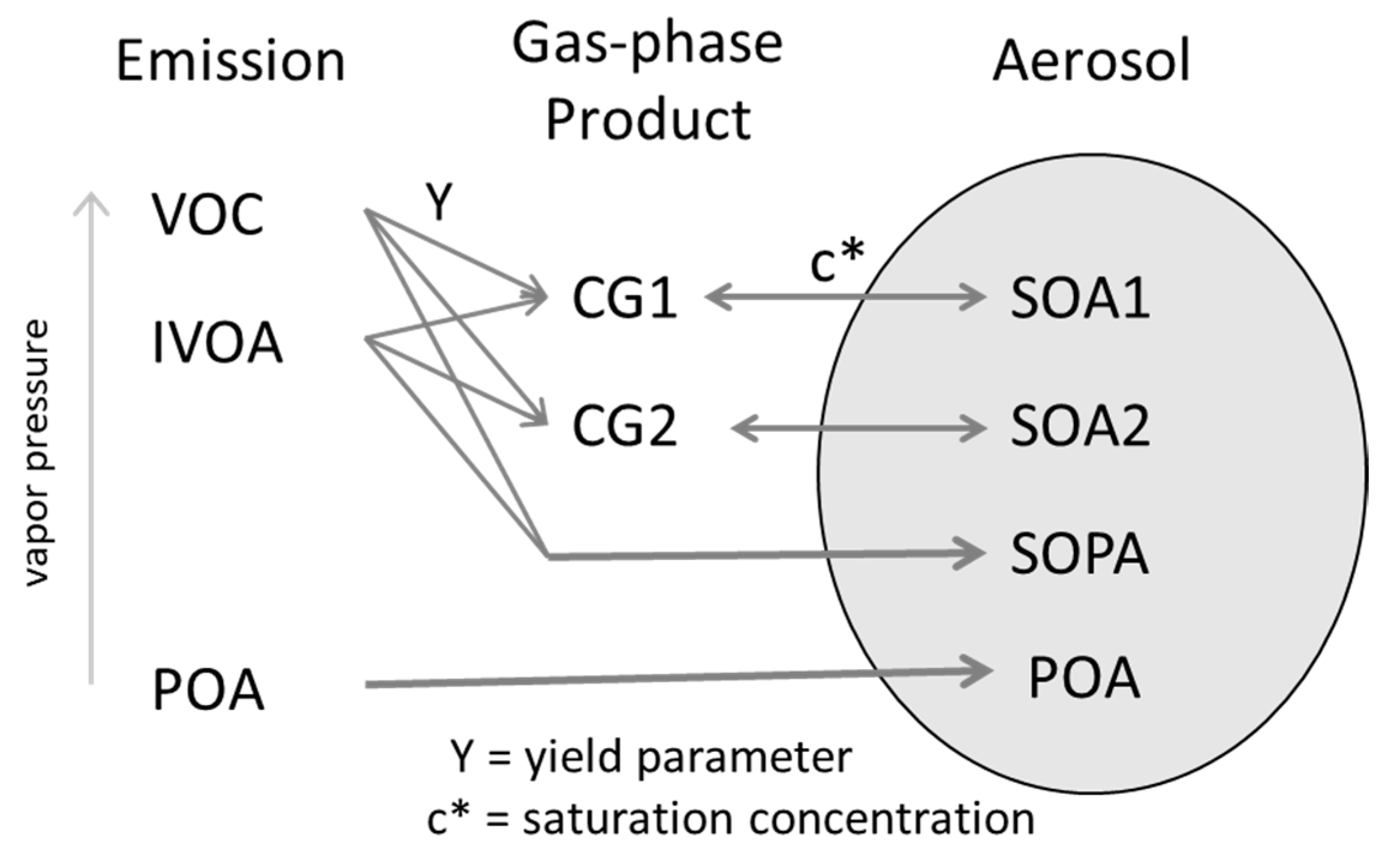
The SOAP module treats the conversion of emitted volatile organic compounds (VOCs) and intermediate volatile organic compounds (IVOCs or IVOAs) to SOA (Figure 4). The module consists of two parts: gas-phase VOC oxidation chemistry that forms condensable gas (CG) products, and equilibrium partitioning between gas and aerosol phases for each CG/SOA pair. Directly emitted (primary) organic aerosol (POA) is considered to be non-volatile and does not chemically evolve. However, POA does influence the chemical evolution of SOA.
Three anthropogenic VOCs (benzene, toluene, and xylene) produce two CG species classified as more-volatile (CG1) and less-volatile (CG2). Likewise, three biogenic VOCs (isoprene, monoterpene, and sesquiterpene) produce two CG species (CG3 and CG4). Non-volatile SOA oxidation products can also be formed (SOPA and SOPB from anthropogenic and biogenic precursors, respectively). Table 3 lists the chemical parameters defined for the SOAP scheme, which are based on aerosol yield data that correct for vapor wall losses in smog chamber experiments [95,96], except for monoterpene yields, which are based on the work of Pye et al. [97,98]. The water solubility of the CG species is modeled based on a parameterization of volatility-dependent Henry’s law constants [99,100].
The SOAP scheme includes the photolytic loss of SOA, which can be competitive with other aging mechanisms of atmospheric SOA [96,101]. This particle-phase removal process is implemented as a first-order decay reaction with a photolysis rate derived by scaling the NO2 photolysis rate based on the work of Malecha et al. [102]. Significant uncertainties in the SOA photolysis rate remain with estimates varying by orders of magnitude [96,101]. In-cloud SOA formation by the RADM-AQ module is added to SOPB. Anthropogenic emissions of IVOCs must be provided separately from the VOC emissions prepared for the oxidant chemistry mechanism (CB or SAPRC). Current emission inventories are generally missing IVOC emissions. Users can omit them or estimate them from emissions of other compounds.
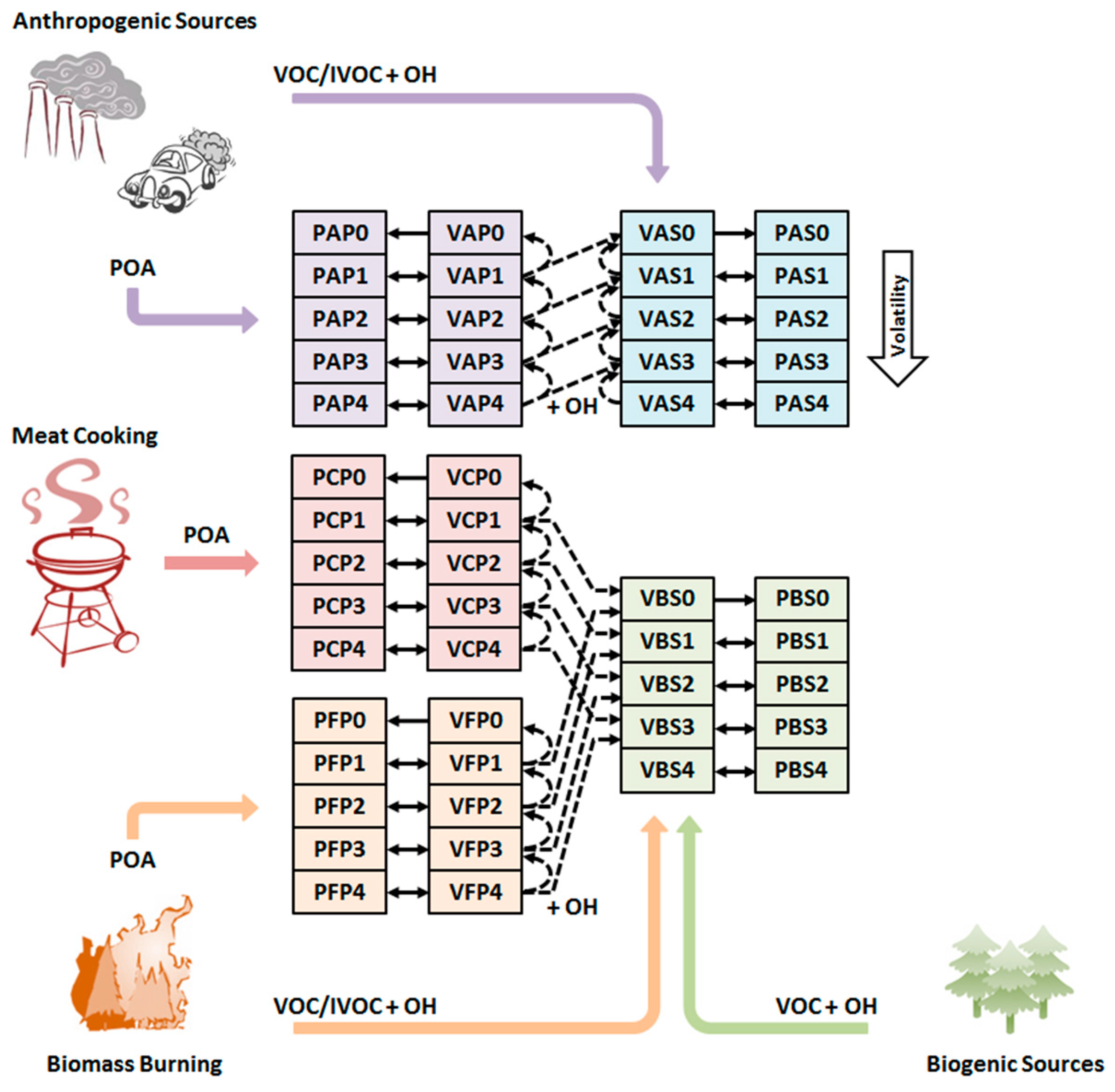
The VBS approach [103,104] provides a unified framework for gas–aerosol partitioning and the chemical aging of both POA and SOA. It uses a set of semi-volatile species with volatility equally spaced in a logarithmic scale (the basis set). VBS member species are allowed to react further in the atmosphere (chemical aging) to describe volatility changes (i.e., the shifting between volatility bins). First generation VBS models use one-dimensional basis sets (1D VBS) wherein organic compounds are grouped only by volatility and thus are unable to describe the varying degrees of oxidation observed in atmospheric organic aerosols (OAs) of similar volatility. To overcome this shortcoming, a two-dimensional VBS (2D VBS) was developed where organic compounds are grouped by oxidation state as well as volatility [105,106]. However, the use of 2D VBS in PGMs has been limited due to the high computational cost.
A hybrid VBS approach is implemented in CAMx (1.5-D VBS), which combines the simplicity of the 1D VBS with the ability to describe the evolution of OA in the 2D space of oxidation state and volatility [45]. This scheme uses five basis sets to describe varying degrees of oxidation in ambient OA: two basis sets for chemically aged, oxygenated OA (anthropogenic and biogenic) and three for freshly emitted OA (meat-cooking, other anthropogenic sources such as exhaust, and biomass burning). A simplified schematic of a VBS is shown in Figure 5.

3. Model Application and Evaluation

Here, we demonstrate an example of predicted regional and seasonal ozone and PM2.5 by summarizing a model evaluation from a recent 2016 national-scale CAMx application. The modeling was conducted by the EPA using input environmental and emission datasets developed to support national air quality assessments and regulatory actions. This evaluation therefore provides a holistic characterization of the entire modeling system specific to this application, inclusive of the PGM, the full complement of input datasets, and other models from which they were developed.
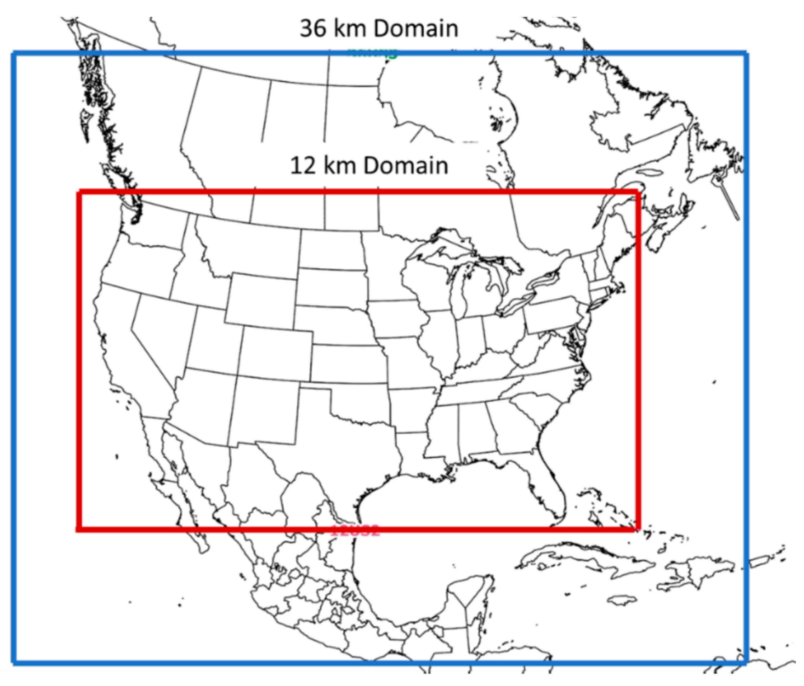
CAMx v7.20 was run over the conterminous 48 US states for the entire year of 2016 using emissions, meteorology, initial/boundary conditions, and photolysis data developed by the EPA [10,11] and references therein. Specifically, all CAMx input datasets were based on the EPA’s 2016 version 3 modeling platform (MP); details on input development are described in the cited references. Gridded and point emission inputs from the most recent 2016v3 MP (referred to as 2016gf_16j [11]) included hourly, speciated, spatially allocated contributions from all anthropogenic, biogenic, fire, oceanic, dust, and lightning NOx sources within the conterminous US and portions of Canada and Mexico within the modeling domains shown in Figure 6. The EPA [10] developed meteorology using WRF v3.8 and developed initial/boundary conditions from a 2016 application of the GEOS-Chem global chemistry model [107] (https://geoschem.github.io/, accessed 14 August 2024). The hourly output from GEOS-Chem defined dynamic boundary conditions for the larger North American modeling grid with 36 km of grid spacing is shown in Figure 6. The EPA ran CAMx on that grid and extracted results to define dynamic boundary conditions for the smaller US modeling grid with 12 km of grid spacing (referred to hereafter as 12US2). For the application described here, we ran CAMx on the single 12US2 modeling domain.
Table 4 lists the CAMx runtime configuration, which is typical for US regional modeling applications. CAMx was run twice by invoking and ignoring the bidirectional ammonia scheme. Particulate ammonium nitrate is semi-volatile and sensitive to ambient ammonia and environmental conditions, and so the bidirectional treatment has an important effect on simulated particle nitrate concentrations. It was important to illustrate this sensitivity in the results described below. The sub-grid cloud convection model (CiG) was not invoked because the EPA’s WRF configuration did not employ the MSKF cumulus scheme and so the needed variable fields were not available from WRF to support this option.

3.1. Model Performance Evaluation Methodology

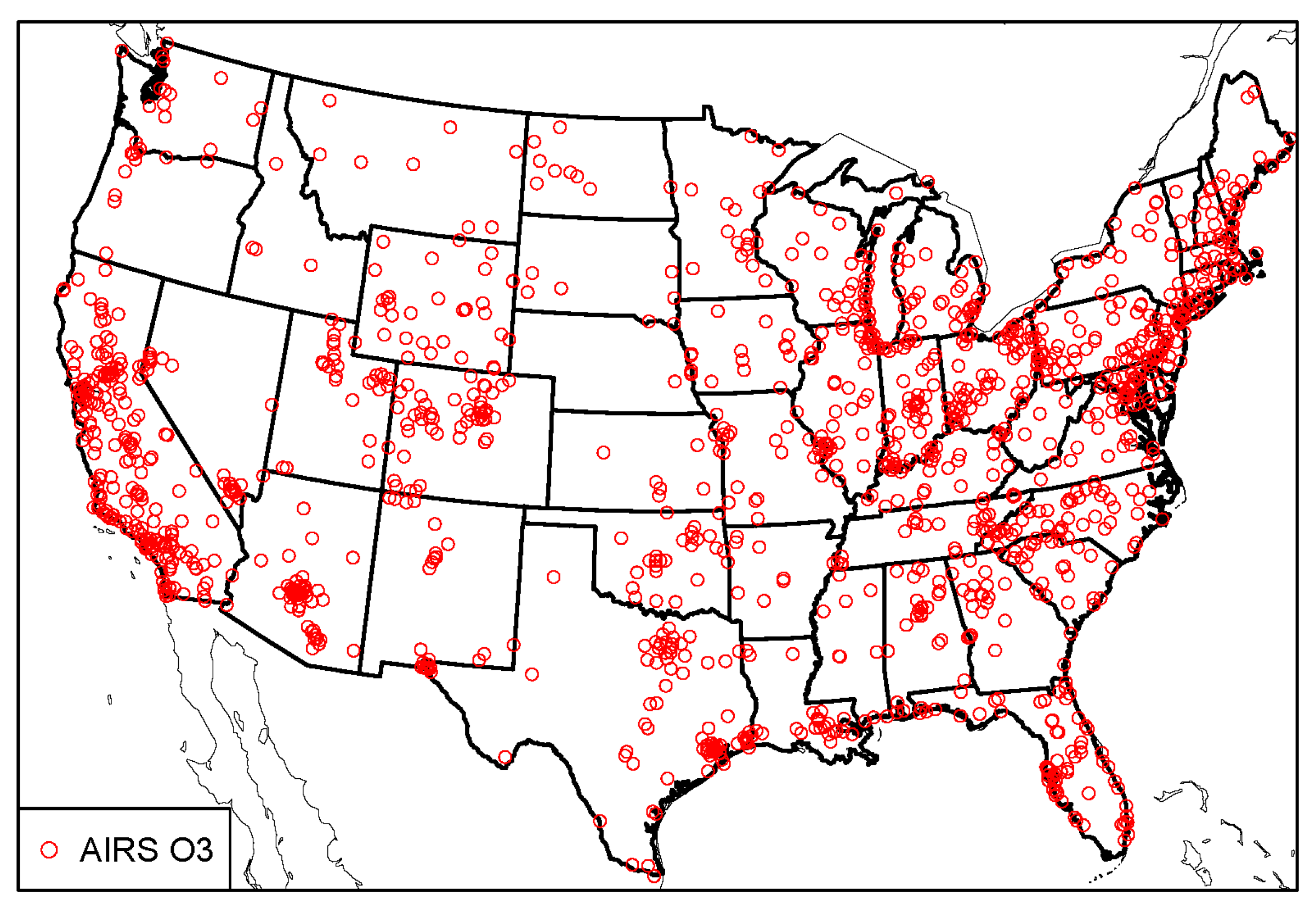
We evaluated model predictions for ozone, PM2.5 constituents, and total PM2.5 mass concentrations against measurements at routine monitoring sites throughout the US to assess model performance in replicating spatial and temporal variability. The US ambient ozone measurement network, referred to as the Air Quality System (AQS; https://www.epa.gov/aqs, accessed on 14 August 2024) or Aerometric Information Retrieval System (AIRS), employs chemiluminescence as the US federal reference method (FRM; 40 CFR part 50, Appendix D, https://www.epa.gov/amtic/final-rulemaking-40-cfr-part-50-appendix-d, accessed on 14 August 2024) and reports ozone concentrations hourly. AQS data are used to determine compliance with the ozone national ambient air quality standard (NAAQS). Figure 7 shows the locations of AQS monitoring sites across the US. The form of the primary ozone NAAQS that protects human health is based on the daily maximum 8 h average (MDA8) ozone concentration, and so model performance is assessed for that specific metric.
Data from four ambient PM monitoring networks were used for the performance evaluation: (1) the Chemical Speciation Network (CSN; https://www.epa.gov/amtic/chemical-speciation-network-csn, accessed on 14 August 2024); (2) the Interagency Monitoring of Protected Visual Environments (IMPROVE) network (http://vista.cira.colostate.edu/Improve/improve-program/, accessed on 14 August 2024); the Clean Air Status and Trends Network (CASTNET; https://www.epa.gov/castnet, accessed on 14 August 2024); and the (4) Ambient Ammonia Monitoring Network (AMON) operated by the National Atmospheric Deposition Program (NADP; https://nadp.slh.wisc.edu/networks/ammonia-monitoring-network/, accessed on 14 August 2024).
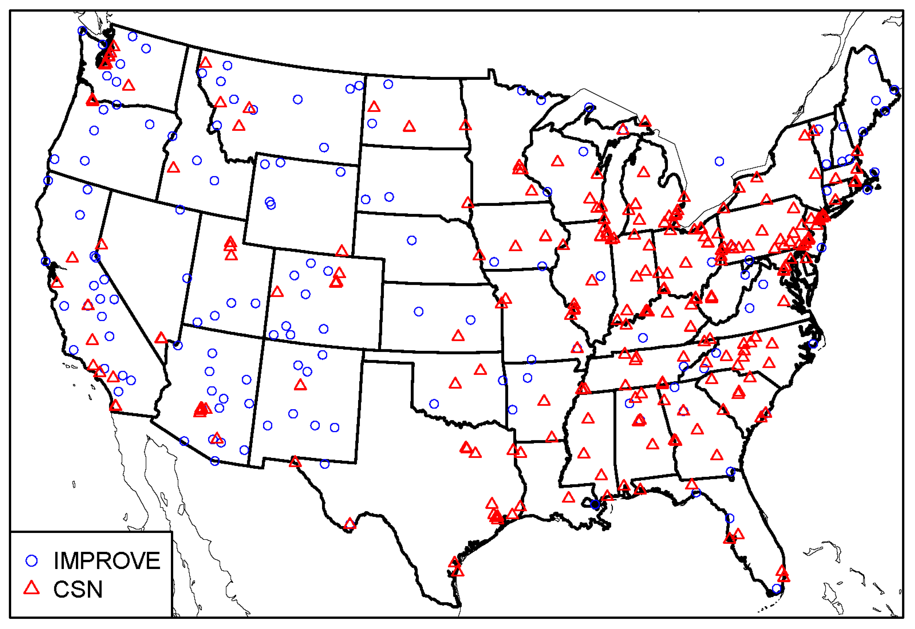
CSN and IMPROVE network site locations are shown in Figure 8. The CSN reports 24 h filter concentrations of sulfate, nitrate, elemental and organic carbon, and the total PM2.5 mass every third or sixth day. CSN data are not used to determined compliance with the PM2.5 NAAQS as filter measurements are not consistent with the PM gravimetric total mass FRM, but rather support scientific and regulatory activities. The IMPROVE network reports 24 h filter samples of sulfate, nitrate, elemental and organic carbon, and the total PM2.5 mass every third day. The IMPROVE program characterizes regional haze/visibility and aerosol conditions and trends in federally protected wildlands including National Parks and Wilderness Areas.
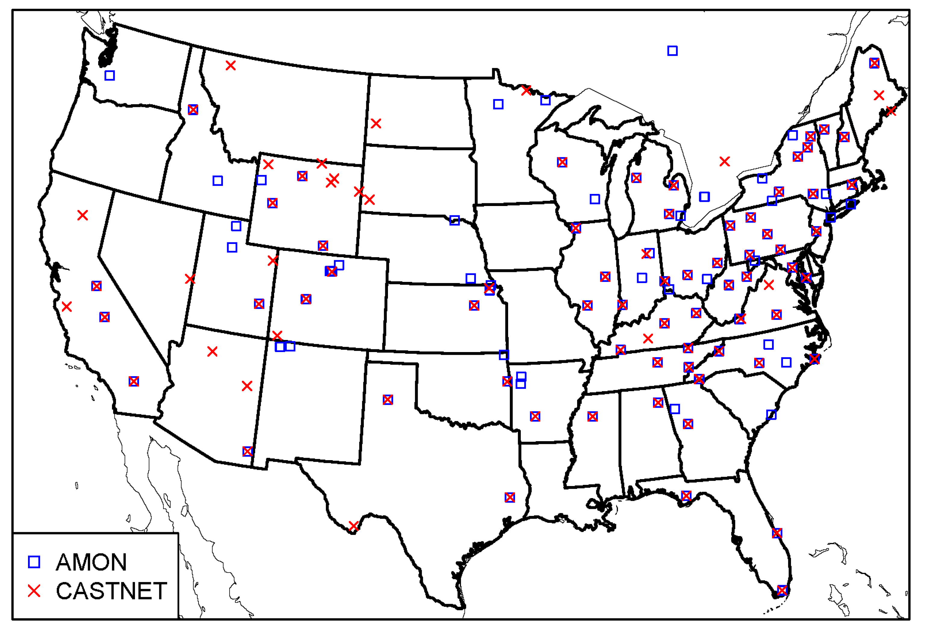
CASTNET and AMON site locations are shown in Figure 9. The CASTNET reports weekly inorganic PM constituent concentrations from filter packs, hourly ozone concentrations from a federal equivalency method, as well as deposition loadings. This study utilized ammonium concentrations from the filter pack measurements. CASTNET and AMON sites are co-located at 70 sites. The AMON reports 2-week average data from passive samplers to characterize trends and spatial variability in ambient NH3 concentrations and deposition. AMON is used to assess atmospheric models and support many other scientific assessments.
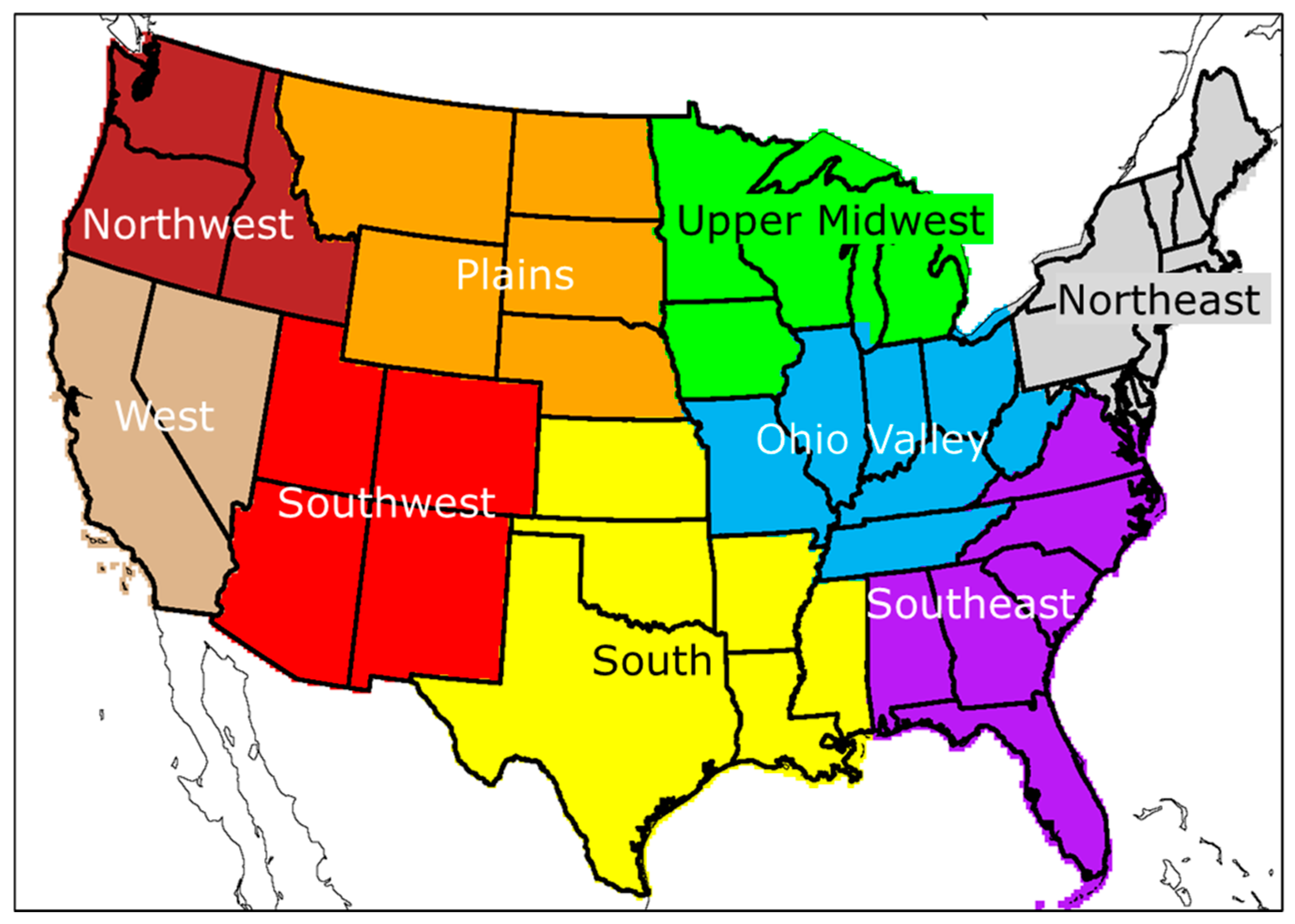
Model predictions were paired with measurements in space and time to support statistical and graphical comparisons. Temporally, our analysis assessed model–measurement agreement by month and over two halves of the year: the cool half (October–March) and the warm half (April–September). Spatially, our analysis aggregated results at monitoring sites over 9 US climate zones (Figure 10) as identified by the US National Oceanic and Atmospheric Administration (NOAA) [108].
Statistical comparisons involved mean bias (MB) and error (ME), normalized bias (NMB) and error (NME), and the Pearson correlation coefficient (r). These particular metrics align with those listed by Simon et al. [109] and Emery et al. [110], the latter of which established benchmarks for well-performing models based on a 10 year history of previous US photochemical modeling applications. The mathematical representation of these metrics is listed below:
M B = 1 N N ( P O )
M E = 1 N N | P O |
N M B = N ( P O ) N O
N M E = N ( P O ) N O
r = N P P ¯ × O O ¯ N P P ¯ 2 × N O O ¯ 2
where P and O are predicted and observed (measured) concentrations, respectively, at each time and site, overbars represent mean quantities over time and site, and summations are over all N times and sites. MB and ME are expressed in concentration units (ppb for gasses, µg/m3 for PM), NMB and NME are expressed as percentages, and r is unitless (1 is perfect correlation, 0 is uncorrelated, negative is anticorrelated). Emery et al. [110] proposed ozone and PM2.5 performance criteria for NMB, NME, and r (Table 5), which represent values that about two-thirds of historical US applications have achieved. As such, the criteria benchmarks are meant to provide context for characterizing typical model performance and should not be interpreted as a “pass/fail test”.

3.2. Evaluation for Ozone

Our assessment of modeled ozone concentrations against measurements focuses on the April–September season of 2016 when ozone concentrations are highest due to elevated photolysis rates and warm temperatures. Statistics were created using data on all days with valid measurement data during this period, as well as for the subset of days when measured MDA8 ozone concentrations exceeded 60 ppb. The latter set of statistics is useful to isolate model performance on high days approaching the 2015 ozone NAAQS of 70 ppb, and is an approach recommended in the EPA’s regulatory modeling guidance [111].
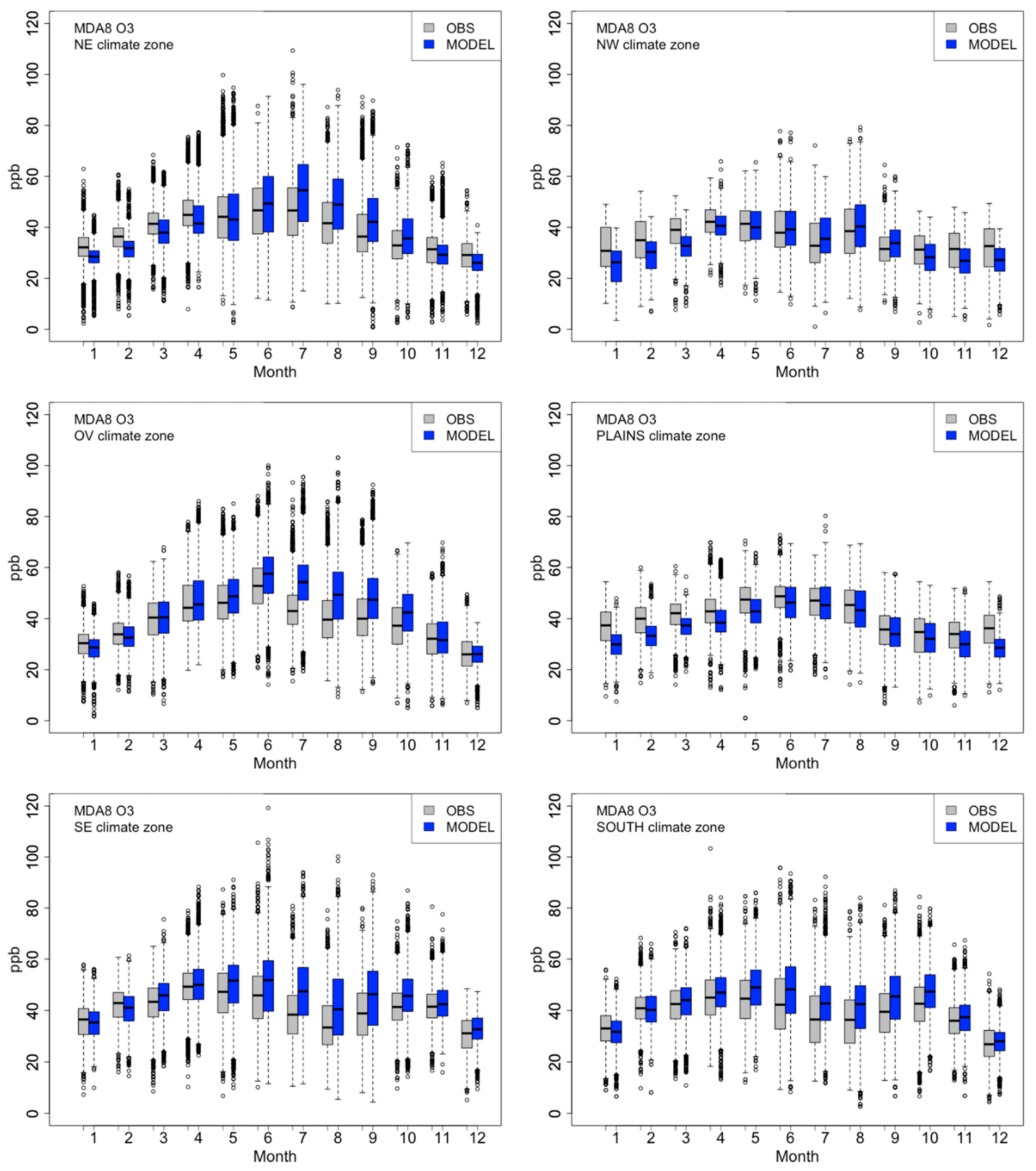
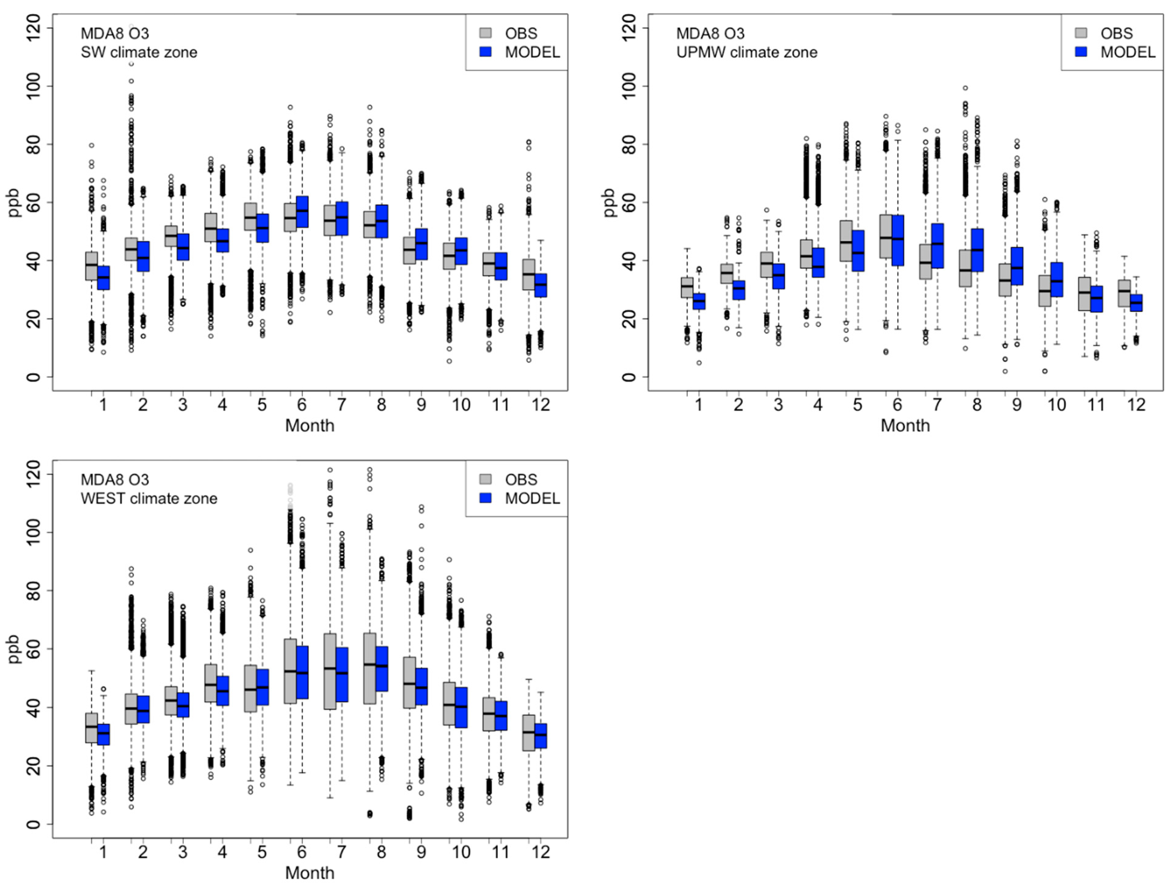
Figure 11 compares monthly box-whisker plots between the observed and simulated MDA8 ozone, separated by US climate zone. These comparisons are unpaired in time and space (other than grouping by climate zone). As we would expect, the model tracks the evolution of MDA8 ozone from the lowest concentration ranges during the winter months through the highest concentration ranges during the summer months. Generally, the model predicts patterns and ranges well for all months and zones, although with a tendency toward the overprediction of the interquartile range. While CAMx captures the tendency for lower mid-summer ozone in the South, Southeast, Upper Midwest, and Ohio Valley, it is not sufficiently low, resulting in larger overpredictions in those areas. Causes for lower mid-summer MDA8 ozone may be related to the higher frequency and extent of smaller-scale afternoon cloud cover and precipitation in those climate zones, a phenomenon that has proven to be difficult for WRF to characterize accurately [58,59,61]. Cloud cover not only impacts photolysis rates but can also reduces biogenic and other temperature-sensitive VOC emissions (e.g., from mobile sources). We note that this phenomenon is not observed nor modeled in dryer climate zones such as the West and Southwest.
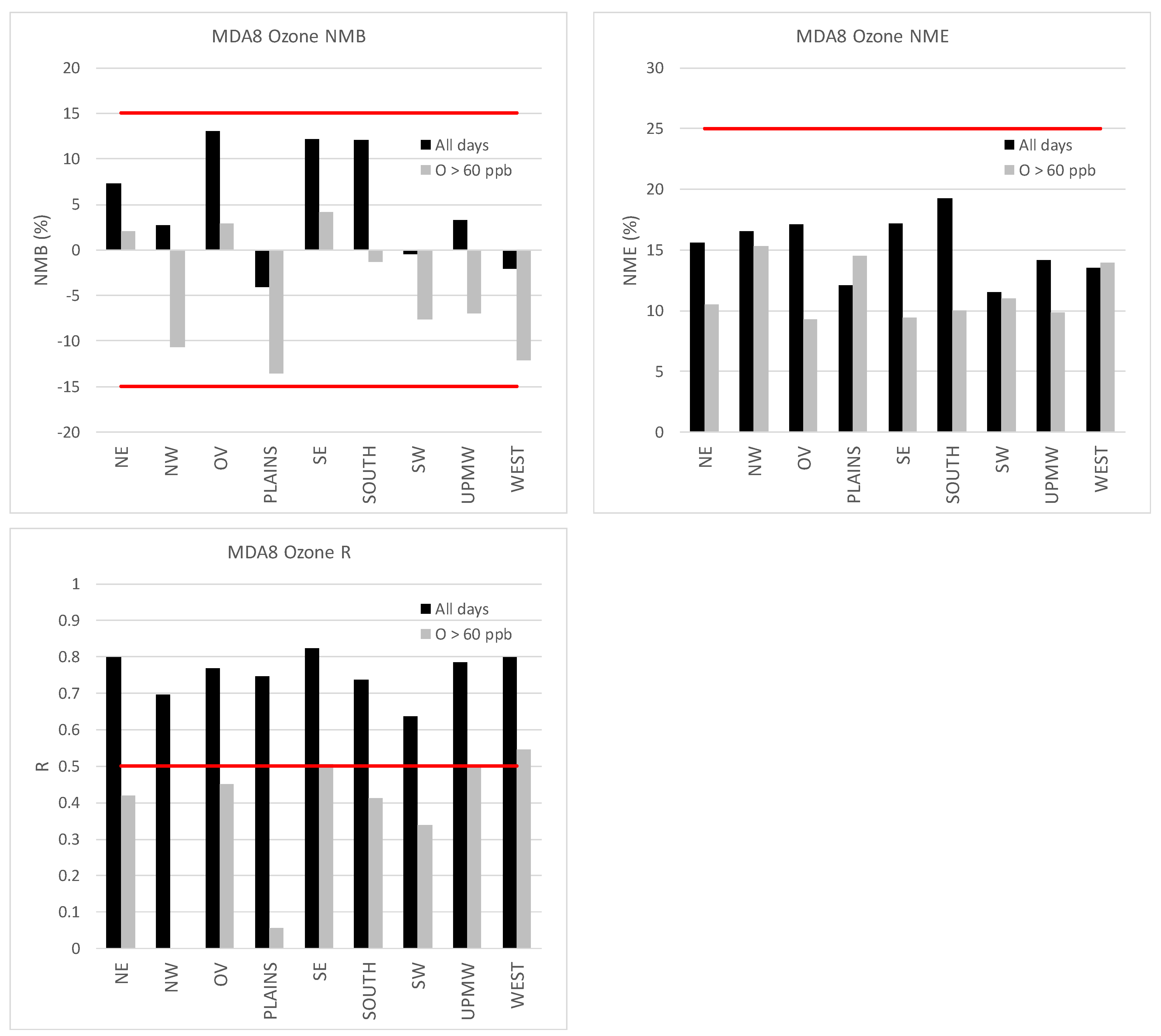
Statistical results from space- and time-paired measured and simulated MDA8 ozone data over the April–September season are summarized in Figure 12. Considering all days in the season, the model performs within criteria benchmarks (shown as red lines) for NMB, NME, and r over all climate zones. The same is true for NMB and NME for the subset of days when the observed MDA8 ozone exceeds 60 ppb, but with a shift toward underprediction. Correlation suffers on such days partly because of a smaller sample size but mainly because of reduced fidelity in matching the highest measurements on a time-paired basis. Additional results are provided in the Supplemental Information, including spatial plots of site-specific, seasonally averaged MDA8 ozone and MB data.

3.3. Evaluation for PM2.5

Our assessment of modeled total and constituent PM2.5 concentrations against measurements includes the April–September and October–March seasons of 2016. Statistics were created using data on all days with valid observed data during these periods. Results presented in this section are consistent with a recent multi-year US-wide PM2.5 model performance evaluation performed by Kelly et al. [112] using the EPA Community Multiscale Air Quality (CMAQ) model [113].
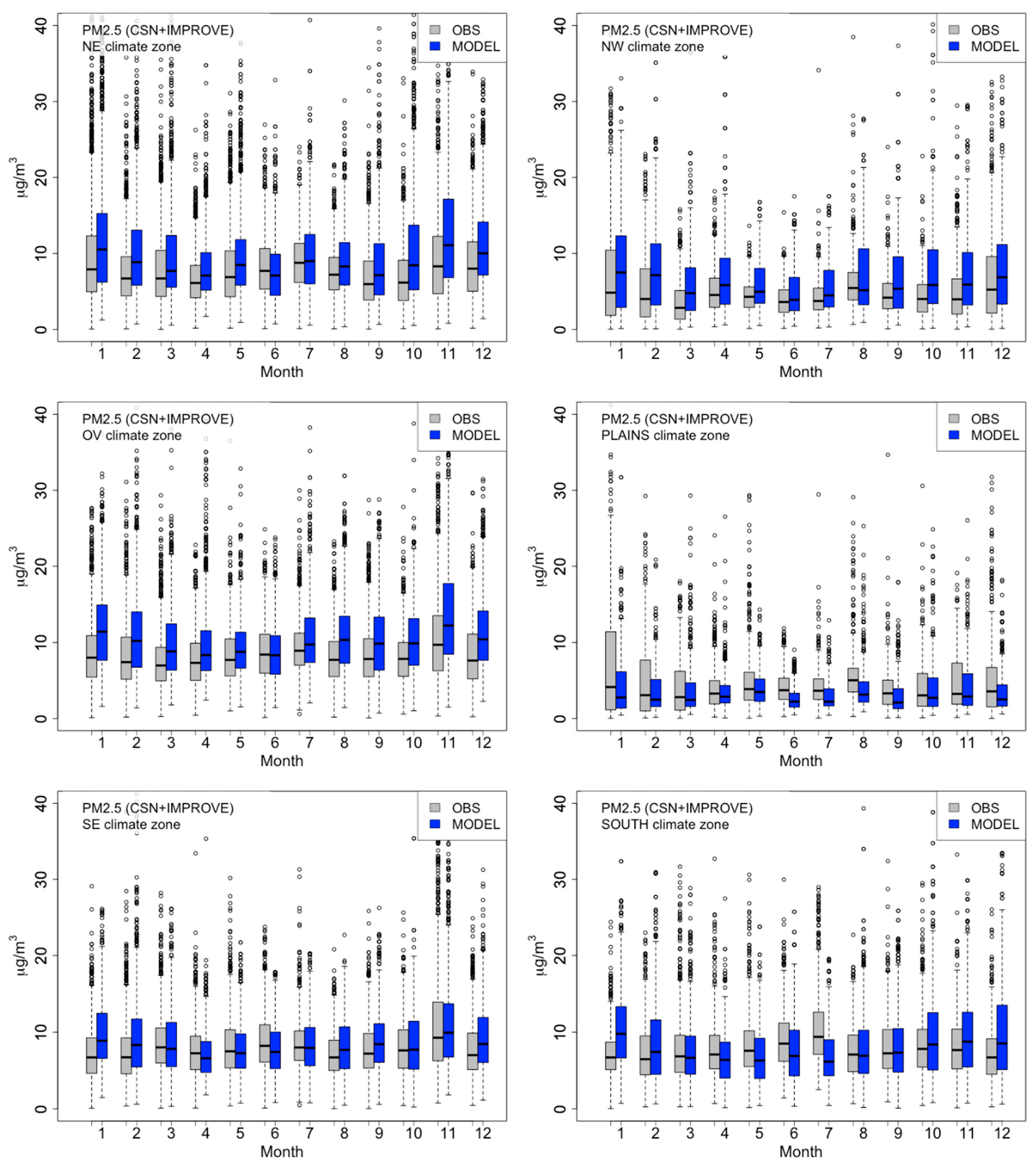
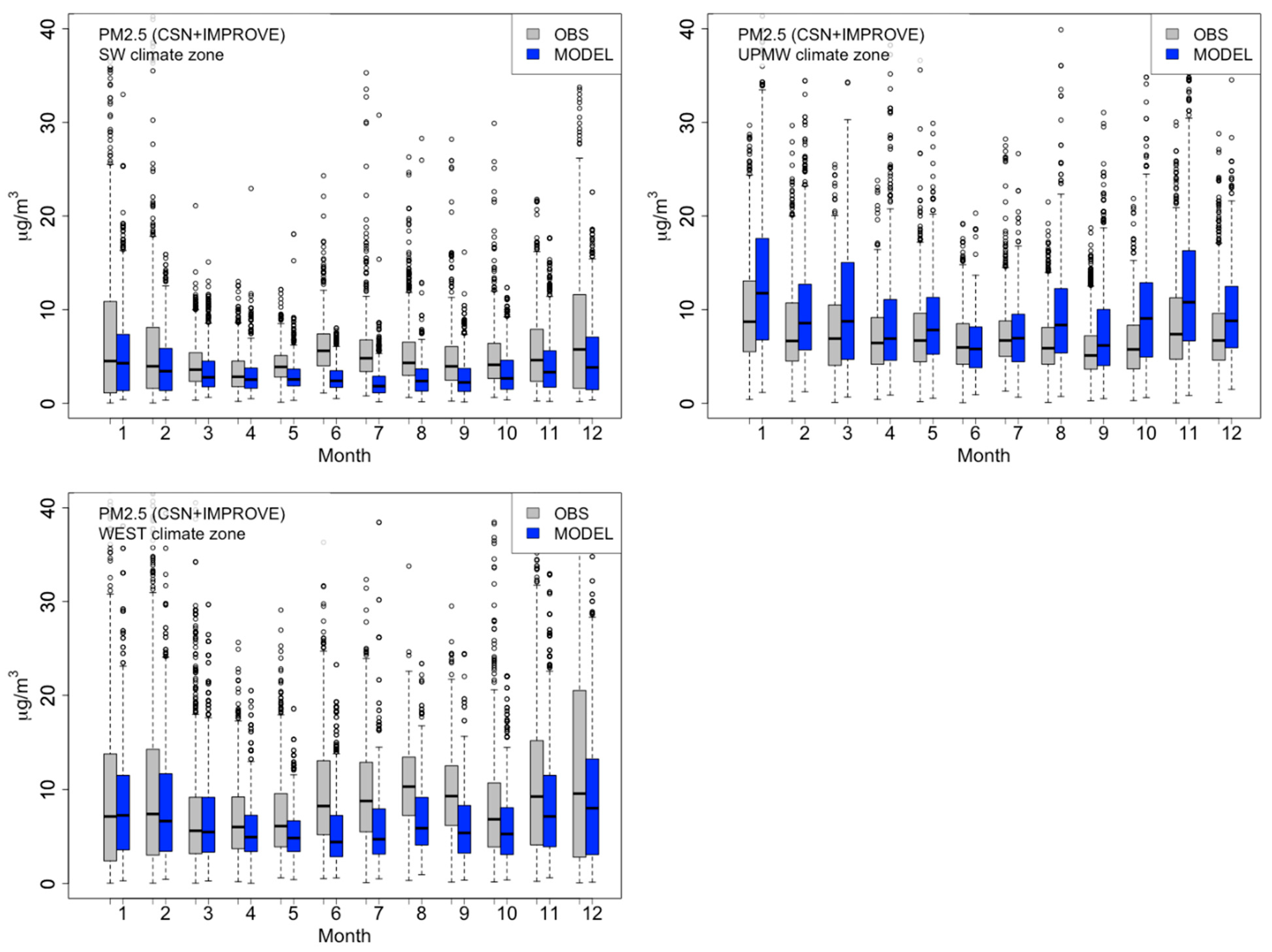
Figure 13 compares monthly box-whisker plots between the observed and simulated 24 h total PM2.5, separated by US climate zone. Results for PM2.5 constituents are shown in the Supplemental Information. The interquartile range of the measured PM2.5 tends to remain fairly constant throughout the year among all zones, with slightly higher concentrations during the winter months. Some areas such as the South, Southwest, and West also experience relatively higher concentrations in mid-summer. More notably, outlier concentrations amplify these trends, with the highest concentrations often occurring during January and December and in mid-summer. Generally, the model captures these patterns well, with a tendency for slight overpredictions in most areas but underpredictions in the Plains, South, Southwest and West during the mid-summer months. Causes for higher winter concentrations are related to more stable, less-ventilated meteorological episodes that trap PM2.5, as well as the increased partitioning of condensable gasses such as nitrate and organics into the particle phase in the more prevalent cool, moist conditions [112]. Conversely, causes for higher summer concentrations are related to elevated chemical production rates, higher evaporative emissions from mobile and biogenic sources, and increased fire activity [114,115].
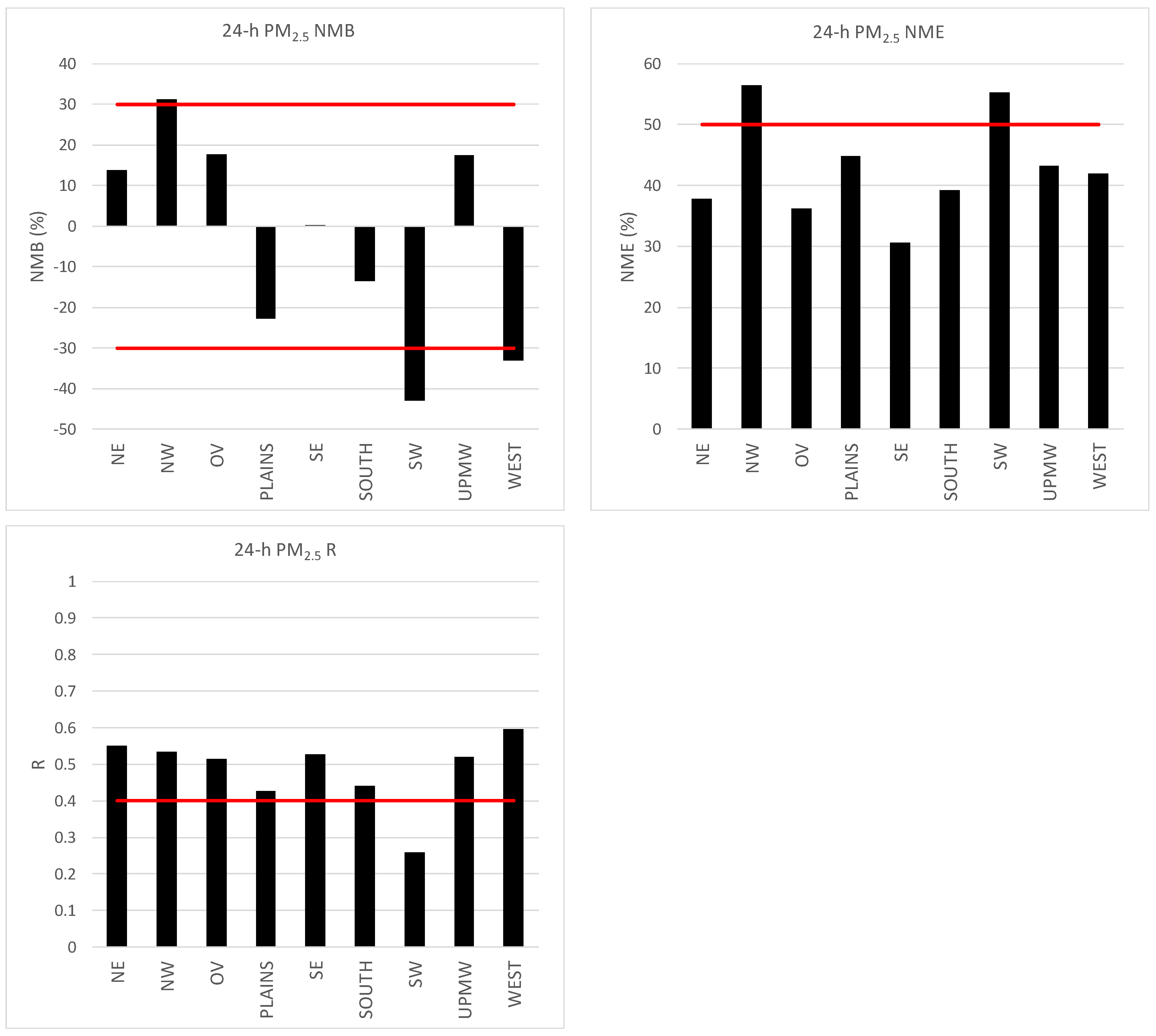
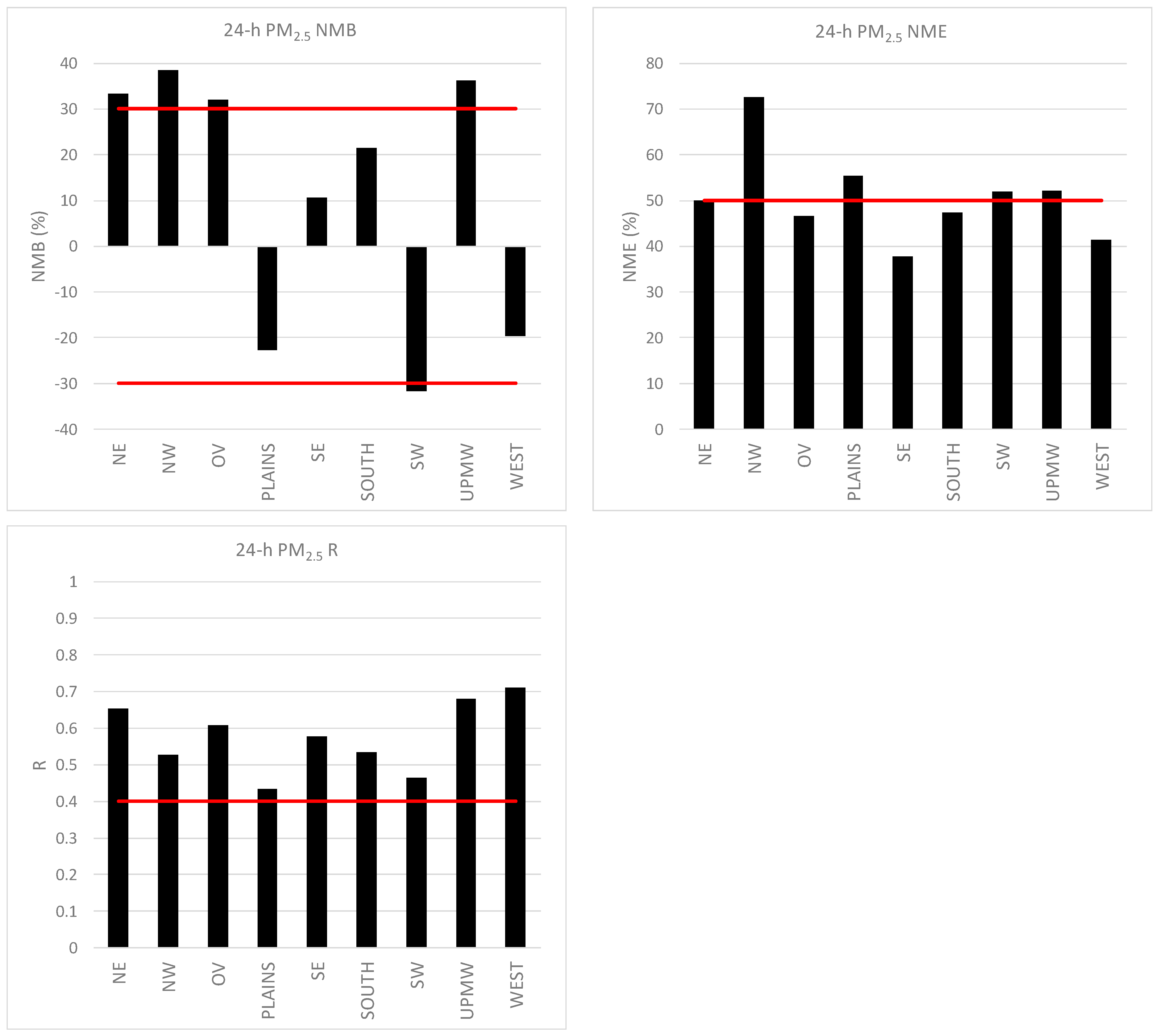
Statistical results from space- and time-paired measured and simulated 24 h total PM2.5 over the April–September warm season are summarized in Figure 14. Results for the combined January–March/October–December cool season are presented in Figure 15. Results for PM2.5 constituents are shown in the Supplemental Information along with spatial plots of site-specific, seasonally averaged 24 h total and constituent PM2.5 and their respective MB. Simulated PM2.5 comparisons among warm and cool seasons considered key weather factors that most influence PM emissions and concentrations, such as temperature, humidity, boundary layer heights, and precipitation patterns.

3.3.1. Warm Season

Figure 14 shows that for total PM2.5, the model performs within criteria benchmarks for NMB in all but three areas (Northwest, Southwest, and West), better than criteria for NME in all but two areas (Northwest and Southwest), and within criteria r in all but one area (Southwest). Overall, the model exhibits a balance of PM2.5 over and underpredictions among climate zones. As we describe below, the performance for PM2.5 constituents represents a mix of over- and underpredictions as well, suggesting that a combination of area-specific factors is at play involving different species contributions, emissions, meteorology, and chemistry.
Summer sulfate concentrations are measured and predicted in the range of 1–2 µg/m3 over the entire US, with much lower concentrations below 1 µg/m3 in the Southwest and West (Figure S1). Statistical performance (Figure S2) is varied with some areas within and some areas exceeding criteria benchmarks. The model exhibits overprediction tendencies across the northern US, particularly in the Northwest, and underprediction tendencies across the southern US and West, most notably in the Southwest. Causes for the consistent north–south performance differences are not readily apparent but may be related to meteorological or climate biases entering from the meteorological model. This southern underprediction may be related to a deficiency in sulfate transported from sources outside the US.
The interquartile range of summer nitrate concentrations remain well below 1 µg/m3 and the model mirrors that pattern fairly well in most areas, depending on the NOx emission density and the availability of ammonia (Figure S4). However, the model tends to overpredict nitrate in all areas and it is well outside criteria benchmarks, except in the Southwest and West, where the model performs well yet slightly low (Figure S5). The largest overpredictions occur in areas with major agricultural (NH3) activity, including the Upper Midwest, Ohio Valley, and the Southeast. Since particulate nitrate formation is most often ammonia-limited, the large overpredictions in these areas indicate an overabundance of ammonia. However, thermodynamically particulate nitrate is highly sensitive to ambient conditions such as relative amounts of other acids and cations, temperature, and humidity. Therefore, other systematic errors in precursor NOx, SOx, and cation emissions, transport rates, removal rates, and several meteorological variables can compound and lead to relatively large errors in predicted nitrate concentrations.
The interquartile range of summer ammonium concentrations is 0.5 µg/m3 or less in most areas with outliers rarely exceeding 1 µg/m3 (Figure S7). Much lower concentrations occur in ammonia-lean areas such as the Northwest, Plains, and Southwest. The range of simulated ammonium tends to be overpredicted in areas with higher concentrations and underpredicted in areas with lower concentrations. These patterns of over- and underprediction are very consistent with particulate nitrate, which is consistent with the fact that the latter responds directly to the amount of available ammonia and confirms that ammonium performance is the primary influence on the nitrate results described above.
Five of the nine regions exceed criteria benchmarks for NMB and NME while four regions exhibit very low correlation (Figure S8).
Summer organic carbon concentrations are observed to range mostly within 1–3 µg/m3 over most climate zones except for much lower levels in the Plains and Southwest (Figure S10). The model generally performs well in matching this pattern, with NMB and NME well within criteria benchmarks, although correlations tend to be low for many areas like other PM constituents (Figure S11). The low organic concentrations in the biogenic-lean Plains and Southwest are underpredicted by about 30%, yet concentrations in the biogenic-rich West and Southeast are also underpredicted by about 25%. The complexities associated with organic aerosols extend to their treatment of emissions and chemistry, as well as meteorological factors that influence their volatility. Furthermore, the SOAP algorithm as applied in this simulation ignores important contributions from anthropogenic intermediate- and semi-volatile organic emissions.
Summer elemental carbon concentrations are well-replicated in all climate zones, which remain mostly well below 1 µg/m3 (Figure S13). Statistical results are well within criteria benchmarks, with correlation exceeding 0.5 in all but two areas (Figure S14). This indicates that the modeling system provides a good characterization of primary carbon emission sources and transport/mixing, without chemical complications associated with secondary constituents. The only performance exception is an outlying overprediction in the Northwest, which is generally consistent with results reported by Kelly et al. [112]. Presumably, this feature relates to a combination of unique emission sectors (especially anthropogenic woodsmoke and wildfire activity), however, we would expect fire emissions to drive similar overpredictions of organic carbon, which is not evident in Figure S11. Another possible cause could be a general tendency for inadequate boundary layer mixing or underestimates of rainfall propagated from the meteorological model (factors similarly influencing the sulfate overpredictions described above).

3.3.2. Cool Season

Statistical performance for total PM2.5 degrades relative to the warm season, with NMB and NME at or exceeding criteria benchmarks in five of the nine areas (Figure 15). Interestingly, correlation generally improves slightly during the cool season by 0.1 or more. In this case, the model tends toward more PM2.5 overpredictions, indicating a more singular systematic source of error, or perhaps a set of errors that tend to compound rather than compensate. As we describe below, all PM2.5 constituent concentrations tend to be overpredicted in most areas during the cool season.
Measured sulfate concentrations do not exhibit much of a seasonal dependence and mostly remain within 1–2 µg/m3 over the entire period in most zones (Figure S1). The exceptions are the South, Southwest and West, where observed sulfate is substantially lower in the cool season. The model performs fairly well in replicating these patterns. Like total PM2.5, the statistical performance for sulfate (Figure S3) indicates a consistent overprediction bias, with several areas exceeding criteria benchmarks for NMB and NME, yet generally good correlation. The Northwest, in particular, continues to be a statistical outlier with large positive NMB and NME.
In most areas, the interquartile range of winter nitrate concentrations increases substantially from summer levels (<1 µg/m3) to 1–4 µg/m3, and the model captures that seasonal variability well but with overpredictions in those areas noted earlier with large ammonia emissions (Figure S4). The model tends to exhibit less of a tendency to overpredict nitrate during the cool season from a relative standpoint (normalized bias and error) given the higher measured nitrate concentrations (Figure S6). The Southeast, however, is a major exception, with NMB and NME reaching 200%. Again, excessive ambient ammonia likely plays a key role in the largest nitrate overpredictions.
In most areas with abundant ammonia emissions, the interquartile range of winter ammonium concentrations increases up to several tenths of a µg/m3 over summer values, and outliers can reach above 2 µg/m3. Exceptions include areas with low ammonia levels (Northwest, Southwest, and West) where winter ammonia is even lower than summer. The model captures the variability by season and region well, but consistently overpredicts (Figure S7). NMB and NME exceed criteria benchmarks in most areas (Figure S9) whereas correlation is within criteria for all but one region (the Southwest, where ammonium is observed to be quite low). Again, the patterns among the observed and modeled winter ammonia concentrations and biases are all consistent with the nitrate performance described above, confirming that excessive ambient ammonia plays a key role in influencing nitrate overpredictions.
Like for sulfate, measured organic carbon concentrations do not vary much seasonally, remaining within 1–3 µg/m3 over most climate zones, except for the lower values in the Plains and Southwest as described earlier (Figure S10). The model overpredicts organic carbon in most areas, exceeding criteria benchmarks for NMB and NME while slightly improving correlation over summer results (Figure S12).
In the winter, we would expect lower rates of organic oxidation, substantially less biogenic precursors, and relatively higher contributions from anthropogenic primary, low-volatility organic emissions. Therefore, overpredictions for this constituent could be related to overestimates of primary organic emissions, especially due to the lack of partitioning to a semi-volatile form.
Elemental carbon concentrations also exhibit little seasonal variation, remaining below 1 µg/m3 all year long (Figure S13). Statistical results are very similar to warm season results, mostly within criteria benchmarks with higher correlations exceeding 0.6 in all but one area (Figure S15). Again, the Northwest remains an overprediction outlier, likely for similar reasons as those stated early for summer conditions.

3.4. Ammonia Sensitivity to the Bidirectional Scheme

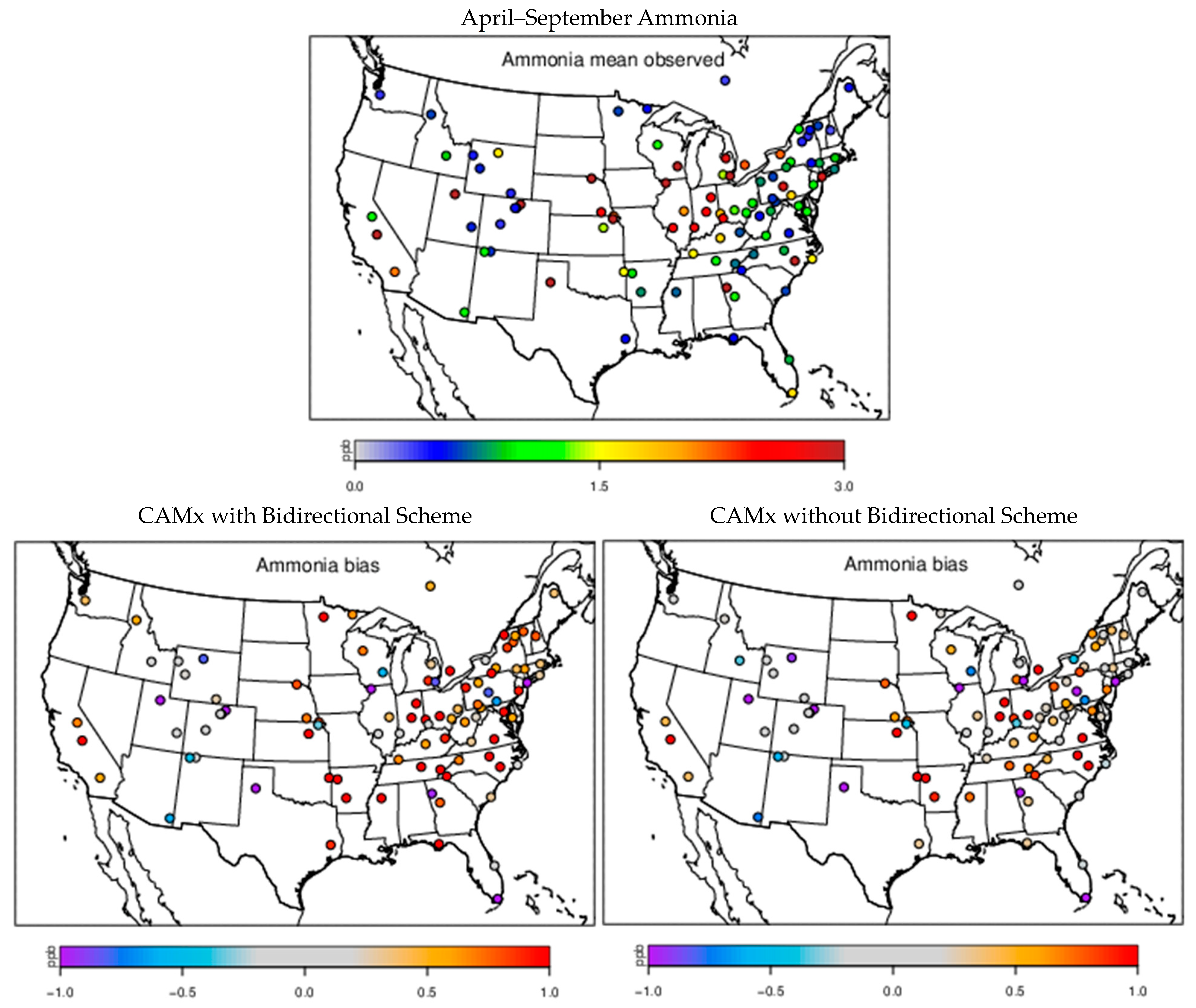
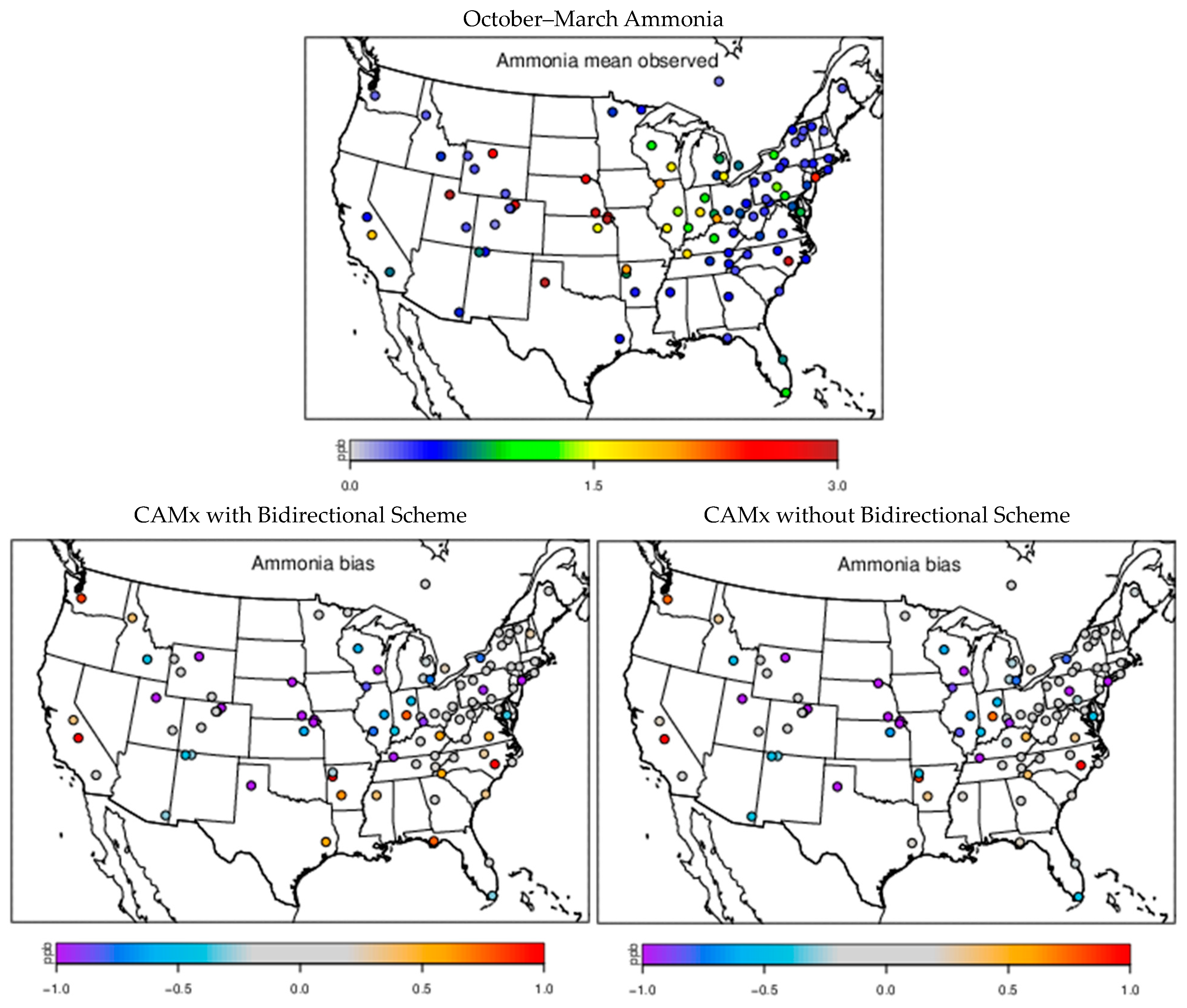
Model performance for particulate nitrate and ammonium hinges in large part on estimates of ammonia emissions, which involve large uncertainty and so are often poorly characterized. We performed two runs of CAMx over the year of 2016, with and without the ammonia bidirectional scheme. Without the bidirectional scheme, only explicit sources of ammonia (agricultural, industrial, residential, etc.) were simulated according to the emission inputs developed by the EPA. With the bidirectional scheme, those same sources were simulated along with additional potential ammonia emissions from natural landcover environments. Figure 16 presents the April–September average observed ammonia and the modeled MB at AMON sites across the US. MB results are shown for CAMx runs with and without the bidirectional scheme. A similar set of plots for October–March is shown in Figure 17.
The pattern of the summer mean of measured ammonia concentrations correlates with agricultural activity across the US. The highest concentrations coincide with areas of intense agriculture, including the Ohio Valley, Plains, and California. The lowest concentrations coincide with areas of the least amount of agriculture, including the Northeast, the Appalachian and Rocky Mountains, and the upper Northwest. Similar spatial patterns are measured during the winter but with a noticeable reduction in concentration levels as snowfall accumulates and agricultural and natural biological/bacterial activities subside.
There is a strong tendency for CAMx to overpredict ammonia during the warm season across the entire US when invoking the bidirectional scheme. The only exceptions occur in the Rocky Mountains, where MB is near zero. Impacts to MB are hardly noticeable when the bidirectional scheme is deactivated, with some reductions at rural sites along the Appalachian Mountains, in the Northeast and Northwest, and along the Gulf Coast. These results are consistent with the CAMx bidirectional methodology, which applies only to natural lands and ignores bidirectional processes over agricultural lands. The apparent lack of any impact in natural areas of the Rocky Mountains indicates that the bidirectional ammonia compensation points for the particular land cover types in that region are appropriately low relative to simulated ambient concentrations (i.e., only deposition is active). On the other hand, the improved MB in other natural areas of the US achieved by deactivating the bidirectional scheme suggests that compensation points for those land cover types are too high relative to simulated ammonia concentrations (i.e., re-emission is overstated).
Modeled ammonia MB is improved during the cool season, with values near zero for a majority of sites. However, there is a slightly stronger tendency toward underpredictions at many sites in Midwest agricultural areas that were uniformly overpredicted during summer. Overall, the bidirectional scheme has much less influence on ammonia concentrations during this season, as shown by virtually identical MB patterns, which is consistent with lower emissions rates and ambient concentrations.

4. Conclusions

We have described the technical formulation of the core processes comprising CAMx v7.20, including pollutant emissions, transport, chemistry, and removal. We examined model spatial and seasonal performance in simulating seasonal ozone and PM2.5 air quality relative to routine monitoring data collected by various US agencies over the conterminous US. Overall, the model performs similarly to its v7 predecessors when applied using the EPA 2016 North American Modeling Platform. Statistical performance for warm season MDA8 ozone was consistently within benchmark statistical criteria for bias, gross error, and correlation over all climate zones, and often near statistical goals [110]. Patterns in the model vs. the measured PM2.5 bias and error analyzed here are consistent with a multi-year evaluation of the CMAQ PGM conducted by the EPA [112] that employed the same domain and similar chemical treatments and input datasets. Statistical performance for 24 h PM2.5 and constituents was more varied than ozone but remained within or near statistical goals except for some outlier seasons, regions, and species. This variability reflects seasonal and regional factors and different sources of uncertainty among PM2.5 species, such as weather influences (e.g., temperature, humidity, boundary layer mixing, clouds and precipitation), chemical treatments and interactions (e.g., ammonia), and emission estimates (e.g., fires).
CAMx v7.20 sets the foundation for several forthcoming major updates currently being implemented for future public releases in 2024–2025. These will be described and evaluated in future publications. The CB6r5 gas-phase mechanism will be expanded to include a modern full halogen reaction set, which is important for certain areas where heavy industrial halogen sources and/or natural saltwater bodies impact local oxidant chemistry. A fundamental update to the Carbon Bond mechanism (CB7) will be added that focuses on the ozone chemistry of biogenic VOCs [116] with more explicit terpene reactions. More explicit chemistry for volatile chemical products (VCPs) will be implemented [117], which are becoming the dominant anthropogenic VOC source [118] as conventional VOC emission categories have been controlled. We will introduce the Regional Atmospheric Chemistry Mechanism, version 2 (RACM2) [119] and the 2022 version of SAPRC [120] to flexibly offer alternative gas-phase mechanisms. The SOAP organic aerosol partitioning scheme will be updated to include semi-volatile primary organic aerosols from anthropogenic sources with parameterized evaporation factors and updated gas–aerosol yields developed from VBS schemes [121]. These state-of-the-science updates are important to address key deficiencies in the current SOAP scheme and accommodate imminent improvements in characterizing intermediate and semi-volatile organic emissions, while maintaining sufficient flexibility and efficiency for multi-scale applications. Finally, CAMx distributed memory parallelization will be updated to accommodate parallel I/O to improve runtime scalability on high performance computer systems.

Supplementary Materials

The following supporting information can be downloaded at: https://www.mdpi.com/article/10.3390/atmos15101158/s1, Figures S1–S23: Species and reaction listings for all CAMx v7.20 gas-phase chemistry mechanisms. Table S1. Reactions and rate constant expressions for the CB6r2 mechanism. See Table S2 for species names. k298 is the rate constant at 298 K and 1 atmosphere using units in cm3 molecule−1 s−1. For photolysis reactions k298 shows the photolysis rate at a solar zenith angle of 60° and height of 600 m MSL/AGL. Table S2. Species names and descriptions for CB6 mechanisms. Table S3. Reactions and rate constant expressions for the CB6r2h halogen mechanism (see Table S1 for a complete listing of CB6r2). See Tables S2 and S4 for species names. k298 is the rate constant at 298 K and 1 atmosphere using units in cm3 molecule−1 s−1. For photolysis reactions k298 shows the photolysis rate at a solar zenith angle of 60° and height of 600 m MSL/AGL. Table S4. Halogen species names and descriptions for CB6r2h. Table S5. Reactions and rate constant expressions for the CB6r4 mechanism. See Table S2 for species names. k298 is the rate constant at 298 K and 1 atmosphere using units in cm3 molecule−1 s−1. For photolysis reactions k298 shows the photolysis rate at a solar zenith angle of 60° and height of 600 m MSL/AGL. Table S6. Reactions and rate constant expressions for the CB6r5 mechanism. See Table S2 for species names. k298 is the rate constant at 298 K and 1 atmosphere using units in cm3 molecule−1 s−1. For photolysis reactions k298 shows the photolysis rate at a solar zenith angle of 60° and height of 600 m MSL/AGL. Table S7. Reactions and rate constants for the SAPRC07TC mechanism. See Table S8 for species names. k300 is the rate constant at 300 K and 1 atmosphere using units in cm3 molecule−1 s−1. For photolysis reactions k298 shows the photolysis rate at a solar zenith angle of 60° and height of 600 m MSL/AGL. Table S8. Species names and descriptions the SAPRC07TC mechanism in CAMx.

Author Contributions

Conceptualization, C.E. and G.Y.; methodology, C.E. and K.B.; CAMx software development, C.E., G.W. and G.Y.; modeling, K.B.; visualization and validation, K.B.; analysis, C.E. and K.B.; writing—original draft preparation, C.E. All authors have read and agreed to the published version of the manuscript.

Funding

This research received no external funding.

Institutional Review Board Statement

Not applicable.

Informed Consent Statement

Not applicable.

Data Availability Statement

The CAMx v7.20 code, open-source user license, release notes, and user guide documentation are publicly and freely distributed at https://www.camx.com/download/source/ (accessed on 14 August 2024). CAMx pre- and post-processing software are publicly and freely distributed at https://www.camx.com/download/support-software/ (accessed on 14 August 2024). The EPA 2016v3 Modeling Platform emissions, boundary conditions, and other ancillary CAMx inputs are publicly available at https://2016v3platform.s3.amazonaws.com/index.html#2016v3platform/ (accessed on 14 August 2024). The EPA 2016v3 Modeling Platform meteorological input files are publicly available at https://views.cira.colostate.edu/iwdw/RequestData/Default.aspx?pid=NEIC_2016_V1 (accessed on 14 August 2024). This website requires a free login account to access the files, which is used only as a security measure for the website and is not used for any marketing purposes. The CAMx model run script for both the baseline and sensitivity simulation as well as the model output files are openly available at https://gaftp.epa.gov/aqmg/baker/emery2024/ (accessed on 14 August 2024).

Acknowledgments

The authors thank the U.S. Environmental Protection Agency for access to the 2016v3 Modeling Platform datasets and the application of CAMx on their Atmos High Performance Computing cluster.

Conflicts of Interest

Christopher Emery, Gary Wilson, and Greg Yarwood are employees of Ramboll Americas Engineering Solutions, Inc. The company had no role in the design of the study; in the collection, analysis, or interpretation of data; in the writing of the manuscript; or in the decision to publish the article. The paper reflects the views of the scientists and not the company. Kirk Baker is an employee of the US Environmental Protection Agency (EPA). The Agency had no roles in the design of the study; in the collection, analysis, or interpretation of data; in the writing of the manuscript; or in the decision to publish the article. The views expressed in this article are those of the authors and do not necessarily represent the views or policies of the Agency. It has been subjected to the Agency’s review and has been approved for publication. Note that approval does not signify that the contents necessarily reflect the views of the Agency.

References

  1. Seinfeld, J.H.; Pandis, S.N. Atmospheric Chemistry and Physics, From Air Pollution to Climate Change; John Wiley and Sons, Inc.: New York, NY, USA, 1998. [Google Scholar]
  2. Guttikunda, S.K.; Jawahar, P. Atmospheric emissions and pollution from the coal-fired thermal power plants in India. Atmos. Environ. 2014, 92, 449–460. [Google Scholar] [CrossRef]
  3. Huszar, P.; Bartík, L.; Karlický, J.; Villalba-Pradas, A. Impact of urbanization on fine particulate matter concentrations over central Europe. Atmos. Chem. Phys. 2024, 24, 397–425. [Google Scholar] [CrossRef]
  4. Basla, B.; Agresti, V.; Balzarini, A.; Giani, P.; Pirovano, G.; Gilardoni, S.; Paglione, M.; Colombi, C.; Belis, C.A.; Poluzzi, V.; et al. Simulations of organic aerosol with CAMx over the Po Valley during the summer season. Atmosphere 2022, 13, 1996. [Google Scholar] [CrossRef]
  5. Garland, R.M.; Naidoo, M.; Sibiya, B.; Naidoo, S.; Bird, T.; von Gruenewaldt, R.; Liebenberg-Enslin, H.; Nekhwalivhe, M.; Netshandama, J.; Mahlatji, M. Importance and Challenges in Use and Uptake of Air Quality Modelling in Developing Countries: Use of CAMx for Air Quality Management in the City of Johannesburg. In AGU Fall Meeting Abstracts; American Geophysical Union: Washington, DC, USA, 2017; Volume 2017, p. A32C-07. [Google Scholar]
  6. Li, L.; An, J.; Zhou, M.; Qiao, L.; Zhu, S.; Yan, R.; Ooi, C.G.; Wang, H.; Huang, C.; Huang, L.; et al. An integrated source apportionment methodology and its application over the Yangtze River Delta region, China. Environ. Sci. Technol. 2018, 52, 14216–14227. [Google Scholar] [CrossRef]
  7. Du, X.; Tang, W.; Cheng, M.; Zhang, Z.; Li, Y.; Li, Y.; Meng, F. Modeling of spatial and temporal variations of ozone-NOx-VOC sensitivity based on photochemical indicators in China. J. Environ. Sci. 2022, 114, 454–464. [Google Scholar] [CrossRef]
  8. EPA. 2017 National Emission Inventory Based Photochemical Modeling for Sector Specific Air Quality Assessments; EPA-454/R-21-005; US Environmental Protection Agency, Office of Air Quality Planning and Standards: Research Triangle Park, NC, USA, 2021. Available online: https://www.epa.gov/system/files/documents/2021-08/epa-454-r-21-005.pdf (accessed on 12 August 2024).
  9. EPA. Air Quality Modeling Technical Support Document: 2016 CAMx PM2.5 Model Evaluation to Support of EGU Benefits Assessments; US Environmental Protection Agency, Office of Air Quality Planning and Standards: Research Triangle Park, NC, USA, 2022. Available online: https://www.epa.gov/system/files/documents/2023-01/PMmodelperformance_2026fj_NH3Rscale0_Final2.pdf (accessed on 12 August 2024).
  10. EPA. Air Quality Modeling Final Rule, Technical Support Document: 2015 Ozone NAAQS Good Neighbor Plan; US Environmental Protection Agency, Office of Air Quality Planning and Standards: Research Triangle Park, NC, USA, 2023. Available online: https://www.epa.gov/system/files/documents/2023-03/AQ%20Modeling%20Final%20Rule%20TSD.pdf (accessed on 12 August 2024).
  11. EPA. Technical Support Document (TSD): Preparation of Emissions Inventories for the 2016v3 North American Emissions Modeling Platform; EPA 454/B-23-002; US Environmental Protection Agency, Office of Air Quality Planning and Standards: Research Triangle Park, NC, USA, 2023. Available online: https://www.epa.gov/system/files/documents/2023-03/2016v3_EmisMod_TSD_January2023_1.pdf (accessed on 12 August 2024).
  12. EPA. Technical Support Document for EPA’s Updated 2028 Regional Haze Modelling; US Environmental Protection Agency, Office of Air Quality Planning and Standards: Research Triangle Park, NC, USA, 2019. Available online: https://www.epa.gov/sites/default/files/2020-10/documents/updated_2028_regional_haze_modeling-tsd-2019.pdf (accessed on 12 August 2024).
  13. Gao, Z.; Zhou, X. A review of the CAMx, CMAQ, WRF-Chem and NAQPMS models: Application, evaluation and uncertainty factors. Environ. Pollut. 2024, 343, 123183. [Google Scholar] [CrossRef]
  14. Shu, Q.; Napelenok, S.L.; Hutzell, W.T.; Baker, K.R.; Henderson, B.H.; Murphy, B.N.; Hogrefe, C. Comparison of ozone formation attribution techniques in the northeastern United States. Geosci. Model Dev. 2023, 16, 2303–2322. [Google Scholar] [CrossRef]
  15. Itahashi, S.; Yamaji, K.; Chatani, S.; Hisatsune, K.; Saito, S.; Hayami, H. Model Performance Differences in Sulfate Aerosol in Winter over Japan Based on Regional Chemical Transport Models of CMAQ and CAMx. Atmosphere 2018, 9, 488. [Google Scholar] [CrossRef]
  16. Shimadera, H.; Kojima, T.; Kondo, A.; Inoue, Y. Performance comparison of CMAQ and CAMx for one-year PM2.5 simulation in Japan. Int. J. Environ. Pollut. 2015, 57, 146–161. [Google Scholar] [CrossRef]
  17. Ramboll. User’s Guide: Comprehensive Air Quality Model with Extensions, Version 7.20. Available online: www.camx.com (accessed on 12 August 2024).
  18. Arakawa, A.; Lamb, V.R. Computational design of the basic dynamical processes of the UCLA general circulation model. In Methods in Computational Physics; Chang, J., Ed.; Academic Press: Cambridge, MA, USA, 1977; pp. 174–267. [Google Scholar]
  19. Colella, P.; Woodward, P.R. The Piecewise Parabolic Method (PPM) for Gas-dynamical Simulations. J. Comp. Phys. 1984, 54, 174–201. [Google Scholar] [CrossRef]
  20. Odman, M.T.; Ingram, C.L. Multiscale Air Quality Simulation Platform (MAQSIP): Source Code Documentation and Validation; Technical Report (ENV-96TR002); MCNC–North Carolina Supercomputing Center: Research Triangle Park, NC, USA, 1996; 83p. [Google Scholar]
  21. Bott, A. A Positive Definite Advection Scheme Obtained by Nonlinear Renormalization of the Advective Fluxes. Mon. Weather Rev. 1989, 117, 1006–1015. [Google Scholar] [CrossRef]
  22. Emery, C.; Tai, E.; Yarwood, G.; Morris, R. Investigation into approaches to reduce excessive vertical transport over complex terrain in a regional photochemical grid model. Atmos. Environ. 2011, 45, 7341–7351. [Google Scholar] [CrossRef]
  23. Pleim, J. A combined local and nonlocal closure model for the atmospheric boundary layer. Part I: Model description and testing. J. Appl. Met. Clim. 2007, 46, 1383–1395. [Google Scholar] [CrossRef]
  24. Wesely, M.L. Parameterization of surface resistances to gaseous dry deposition in regional-scale numerical models. Atmos. Environ. 1989, 23, 1293–1304. [Google Scholar] [CrossRef]
  25. Zhang, L.; Brook, J.R.; Vet, R. A revised parameterization for gaseous dry deposition in air-quality models. Atmos. Chem. Phys. 2003, 3, 2067–2082. [Google Scholar] [CrossRef]
  26. Slinn, S.A.; Slinn, W.G.N. Predictions for particle deposition on natural waters. Atmos. Environ. 1980, 24, 1013–1016. [Google Scholar] [CrossRef]
  27. Zhang, L.; Gong, S.; Padro, J.; Barrie, L. A size-segregated particle dry deposition scheme for an atmospheric aerosol module. Atmos. Environ. 2001, 35, 549–560. [Google Scholar] [CrossRef]
  28. Zhang, L.; Wright, L.P.; Asman, W.A.H. Bi-directional air-surface exchange of atmospheric ammonia: A review of measurements and a development of a big-leaf model for applications in regional-scale air-quality models. J. Geophys. Res. Atmos. 2010, 115, D20310. [Google Scholar] [CrossRef]
  29. Emery, C.; Johnson, J.; Rasmussen, D.J.; Hsieh, W.C.; Yarwood, G.; Nielsen-Gammon, J.; Bowman, K.; Zhang, R.; Lin, Y.; Siu, L. Development and Evaluation of an Interactive Sub-Grid Cloud Framework for the CAMx Photochemical Model; Prepared for the Texas Air Quality Research Program; University of Texas at Austin: Austin, TX, USA, 2015; Available online: https://people.tamu.edu/~k-bowman/pdf/AQRP_14-025_final_report_31Jul15.pdf (accessed on 30 August 2024).
  30. Yarwood, G.; Jung, J.; Whitten, G.Z.; Heo, G.; Mellberg, J.; Estes, E. Updates to the Carbon Bond mechanism for version 6 (CB6). In Proceedings of the 9th Annual CMAS Conference, Chapel Hill, NC, USA, 11–13 October 2010. [Google Scholar]
  31. Yarwood, G.; Gookyoung, H.; Carter, W.P.L.; Whitten, G.Z. Environmental Chamber Experiments to Evaluate NOx Sinks and Recycling in Atmospheric Chemical Mechanisms; Texas AQRP (Project 10-042); Prepared for the University of Texas at Austin: Austin, TX, USA, 2012. [Google Scholar]
  32. Yarwood, G.; Sakulyanontvittaya, T.; Nopmongcol, U.; Koo, B. Ozone Depletion by Bromine and Iodine over the Gulf of Mexico; Prepared by Ramboll, Novato, CA for the Texas Commission on Environmental Quality: Austin, TX, USA, 2014. [Google Scholar]
  33. Yarwood, G.; Shi, Y.; Beardsley, R. Impact of CB6r5 Mechanism Changes on Air Pollutant Modeling in Texas; Prepared for the Texas Commission on Environmental Quality: Austin, TX, USA, 2020. [Google Scholar]
  34. Hildebrandt Ruiz, L.H.; Yarwood, G. Interactions between Organic Aerosol and NOy: Influence on Oxidant Production; Texas AQRP (Project 12-012); Prepared by Ramboll, Novato, CA for the University of Texas at Austin: Austin, TX, USA, 2013. [Google Scholar]
  35. Emery, C.; Jung, J.; Koo, B.; Yarwood, G. Improvements to CAMx Snow Cover Treatments and Carbon Bond Chemical Mechanism for Winter Ozone, Utah Department of Environmental Quality; Prepared by Ramboll, Novato, CA for the Division of Air Quality: Salt Lake City, UT, USA, 2015. [Google Scholar]
  36. Carter, W.P.L. Development of the SAPRC-07 chemical mechanism. Atmos. Environ. 2010, 44, 5324–5335. [Google Scholar] [CrossRef]
  37. Hutzell, W.T.; Luecken, D.J.; Appel, K.W.; Carter, W.P.L. Interpreting predictions from the SAPRC07 mechanism based on regional and continental simulations. Atmos. Environ. 2012, 46, 417–429. [Google Scholar] [CrossRef]
  38. Hertel, O.; Berkowics, R.; Christensen, J.; Hov, O. Test of two numerical schemes for use in atmospheric transport-chemistry models. Atmos. Environ. 1993, 27, 2591–2611. [Google Scholar] [CrossRef]
  39. Byrne, G.D.; Hindmarsh, A.C. Stiff ODE solvers: A review of current and coming attractions. J. Comput. Phys. 1987, 70, 1–62. [Google Scholar] [CrossRef]
  40. Nenes, A.; Pilinis, C.; Pandis, S.N. ISORROPIA: A new thermodynamic model for multiphase multicomponent inorganic aerosols. Aquat. Geochem. 1998, 4, 123–152. [Google Scholar] [CrossRef]
  41. Nenes, A.; Pilinis, C.; Pandis, S.N. Continued development and testing of a new thermodynamic aerosol module for urban and regional air quality models. Atmos. Environ. 1999, 33, 1553–1560. [Google Scholar] [CrossRef]
  42. Metzger, S.; Steil, B.; Abdelkader, M.; Klingmüller, K.; Xu, L.; Penner, J.E.; Fountoukis, C.; Nenes, A.; Lelieveld, J. Aerosol water parameterisation: A single parameter framework. Atmos. Chem. Phys. 2016, 16, 7213–7237. [Google Scholar] [CrossRef]
  43. Chang, J.S.; Brost, R.A.; Isaksen, I.S.A.; Madronich, S.; Middleton, P.; Stockwell, W.R.; Walcek, C.J. A Three-dimensional Eulerian Acid Deposition Model: Physical Concepts and Formulation. J. Geophys. Res. 1987, 92, 14681–14700. [Google Scholar] [CrossRef]
  44. Strader, R.; Lurmann, F.; Pandis, S.N. Evaluation of secondary organic aerosol formation in winter. Atmos. Environ. 1999, 33, 4849–4863. [Google Scholar] [CrossRef]
  45. Koo, B.; Knipping, E.; Yarwood, G. 1.5-dimensional volatility basis set approach for modeling organic aerosol in CAMx and CMAQ. Atmos. Environ. 2014, 95, 158–164. [Google Scholar] [CrossRef]
  46. Turner, D.B.; Chico, T.; Catalano, A. TUPOS: A Multiple Source Gaussian Dispersion Algorithm Using On-Site Turbulence Data (EPA-600/8-86/010); U.S. Environmental Protection Agency: Research Triangle Park, NC, USA, 1986. Available online: https://cfpub.epa.gov/si/si_public_record_Report.cfm?Lab=ORD&dirEntryID=34599 (accessed on 12 August 2024).
  47. Skamarock, W.C.; Klemp, J.B.; Dudhia, J.; Gill, D.O.; Liu, Z.; Berner, J.; Wang, W.; Powers, J.G.; Duda, M.G.; Barker, D.M.; et al. A Description of the Advanced Research WRF Model Version 4. NCAR Technical Notes (NCAR/TN-556+STR, March 2019). 2019. Available online: https://n2t.org/ark:/85065/d72r3vrp (accessed on 12 August 2024). [CrossRef]
  48. Smagorinsky, J. General circulation experiments with the primitive equations: I. The basic experiment. Mon. Weather Rev. 1963, 91, 99–164. [Google Scholar] [CrossRef]
  49. Anthes, R.A.; Warner, T.T. Development of hydrodynamic models suitable for air pollution and other mesometeorological studies. Mon. Weather Rev. 1978, 106, 1045–1078. [Google Scholar] [CrossRef]
  50. Whaley, C.H.; Makar, P.A.; Shephard, M.W.; Zhang, L.; Zhang, J.; Zheng, Q.; Akingunola, A.; Wentworth, G.R.; Murphy, J.G.; Kharol, S.K.; et al. Contributions of natural and anthropogenic sources to ambient ammonia in the Athabasca Oil Sands and north-western Canada. Atmos. Chem. Phys. 2018, 18, 2011–2034. [Google Scholar] [CrossRef]
  51. Louis, J.F. A parametric model of vertical eddy fluxes in the atmosphere. Bound. Lay. Meteor. 1979, 17, 187–202. [Google Scholar] [CrossRef]
  52. Huebert, B.J.; Robert, C.H. The dry deposition of nitric acid to grass. J. Geophys. Res. 1985, 90, 2085–2090. [Google Scholar] [CrossRef]
  53. Wesely, M.L.; Hicks, B.B. A review of the current status of knowledge on dry deposition. Atmos. Environ. 2000, 34, 2261. [Google Scholar] [CrossRef]
  54. Kumar, N.; Lurmann, F.W.; Wexler, A.S.; Pandis, S.; Seinfeld, J.H. Development and application of a three dimensional aerosol model. In Proceedings of the A&WMA Specialty Conference on Computing in Environmental Resource Management, Research Triangle Park, NC, USA, 2–4 December 1996. [Google Scholar]
  55. Sehmel, G.A. Particle and gas deposition, a review. Atmos. Environ. 1980, 14, 983–1011. [Google Scholar] [CrossRef]
  56. Helmig, D.; Lang, E.K.; Bariteau, L.; Boylan, P.; Fairall, C.W.; Ganzeveld, L.; Hare, J.E.; Hueber, J.; Pallandt, M. Atmospheric-ocean ozone fluxes during the TexAQS 2006, STRATUS 2006, GOMECC 2007, GasEx 2008 and AMMA 2008 Cruises. J. Geophys. Res. 2012, 117, D04305. [Google Scholar] [CrossRef]
  57. Kain, J.S. The Kain-Fritsch convective parameterization: An update. J. Appl. Meteor. 2004, 43, 170–181. [Google Scholar] [CrossRef]
  58. Alapaty, K.; Herwehe, J.A.; Otte, T.L.; Nolte, C.G.; Bullock, O.R.; Mallard, M.S.; Kain, J.S.; Dudhia, J. Introducing subgrid-scale cloud feedbacks to radiation for regional meteorological and climate modelling. Geophys. Res. Lett. 2012, 39, L24809. [Google Scholar] [CrossRef]
  59. Herwehe, J.A.; Alapaty, K.; Spero, T.L.; Nolte, C.G. Increasing the credibility of regional climate simulations by introducing subgrid-scale cloud-radiation interactions. J. Geophys. Res. 2014, 119, 5317–5330. [Google Scholar] [CrossRef]
  60. Bullock, O.R.; Alapaty, K.; Herwehe, J.A.; Kain, J.S. A Dynamically Computed Convective Time Scale for the Kain–Fritsch Convective Parameterization Scheme. Mon. Wea. Rev. 2015, 143, 2105–2120. [Google Scholar] [CrossRef]
  61. Zheng, Y.; Alapaty, K.; Herwehe, J.A.; Del Genio, A.D.; Niyogi, D. Improving high-resolution weather forecasts using the Weather Research and Forecasting (WRF) model with an updated Kain–Fritsch Scheme. Mon. Weather Rev. 2016, 144, 833–860. [Google Scholar] [CrossRef]
  62. Scott, B.C. Parameterization of sulfate removal by precipitation. J. Appl. Meteor. 1978, 17, 1375–1389. [Google Scholar] [CrossRef]
  63. Sauter, D.P.; Wang, P.K. An experimental study of the scavenging of aerosol particles by natural snow crystals. J. Atmos. Sci. 1989, 46, 1650–1655. [Google Scholar] [CrossRef]
  64. Gery, M.W.; Whitten, G.Z.; Killus, J.P.; Dodge, M.C. A photochemical kinetics mechanism for urban and regional scale computer modelling. J. Geophys. Res. 1989, 94, 925–956. [Google Scholar]
  65. Sarwar, G.; Luecken, D.; Yarwood, G.; Whitten, G.Z.; Carter, W.P. Impact of an updated carbon bond mechanism on predictions from the CMAQ modeling system: Preliminary assessment. J. Appl. Meteorol. Climatol. 2008, 47, 3–14. [Google Scholar] [CrossRef]
  66. Yarwood, G.; Jung, J.; Nopmongcol, U.; Emery, C. Improving CAMx Performance in Simulating Ozone Transport from the Gulf of Mexico; Prepared by Ramboll, Novato, CA for the Texas Commission on Environmental Quality: Austin, TX, USA, 2012. [Google Scholar]
  67. Tanaka, P.L.; Allen, D.T.; McDonald-Buller, E.C.; Chang, S.; Kimura, Y.; Mullins, C.B.; Yarwood, G.; Neece, J.D. Development of a chlorine mechanism for use in the carbon bond IV chemistry model. J. Geophys. Res. Atmos. 2003, 108, 1984–2012. [Google Scholar] [CrossRef]
  68. Yeh, G.K.; Ziemann, P.J. Alkyl nitrate formation from the reactions of C8–C14 n-alkanes with OH radicals in the presence of NOx: Measured yields with essential corrections for gas–wall partitioning. J. Phys. Chem. 2014, 118, 8797–8806. [Google Scholar] [CrossRef]
  69. Lee, L.; Wooldridge, P.J.; Gilman, J.B.; Warneke, C.; de Gouw, J.; Cohen, R.C. Low temperatures enhance organic nitrate formation: Evidence from observations in the 2012 Uintah Basin Winter Ozone Study. Atmos. Chem. Phys. 2014, 14, 12441–12454. [Google Scholar] [CrossRef]
  70. Perring, A.E.; Pusede, S.E.; Cohen, R.C. An observational perspective on the atmospheric impacts of alkyl and multifunctional nitrates on ozone and secondary organic aerosol. Chem. Rev. 2013, 113, 5848–5870. [Google Scholar] [CrossRef]
  71. Carpenter, L.J.; MacDonald, S.M.; Shaw, M.D.; Kumar, R.; Saunders, R.W.; Parthipan, R.; Wilson, J.; Plane, J.M.C. Atmospheric iodine levels influenced by sea surface emissions of inorganic iodine. Nat. Geosci. 2013, 6, 108–111. [Google Scholar] [CrossRef]
  72. Lamarque, J.F.; Emmons, L.K.; Hess, P.G.; Kinnison, D.E.; Tilmes, S.; Vitt, F.; Heald, C.L.; Holland, E.A.; Lauritzen, P.H.; Neu, J.; et al. CAM-chem: Description and evaluation of interactive atmospheric chemistry in the Community Earth System Model. Geosci. Model. Dev. 2012, 5, 369–411. [Google Scholar] [CrossRef]
  73. Jacobs, M.I.; Burke, W.J.; Elrod, M.J. Kinetics of the reactions of isoprene-derived hydroxynitrates: Gas phase epoxide formation and solution phase hydrolysis. Atmos. Chem. Phys. 2014, 14, 8933–8946. [Google Scholar] [CrossRef]
  74. Fisher, J.A.; Jacob, D.J.; Travis, K.R.; Kim, P.S.; Marais, E.A.; Chan Miller, C.; Yu, K.; Zhu, L.; Yantosca, R.M.; Sulprizio, M.P.; et al. Organic nitrate chemistry and its implications for nitrogen budgets in an isoprene- and monoterpene-rich atmosphere: Constraints from aircraft (SEAC4RS) and ground-based (SOAS) observations in the Southeast US. Atmos. Chem. Phys. 2016, 16, 5969–5991. [Google Scholar] [CrossRef]
  75. Rollins, A.W.; Pusede, S.; Wooldridge, P.; Min, K.-E.; Gentner, D.R.; Goldstein, A.H.; Liu, S.; Day, D.A.; Russell, L.M.; Rubitschun, C.L.; et al. Gas/particle partitioning of total alkyl nitrates observed with TD-LIF in Bakersfield. J. Geophys. Res. Atmos. 2013, 118, 6651–6662. [Google Scholar] [CrossRef]
  76. Burkholder, J.B.; Sander, S.P.; Abbatt, J.P.D.; Barker, J.R.; Cappa, C.; Crounse, J.D.; Dibble, T.S.; Huie, R.E.; Kolb, C.E.; Kurylo, M.J.; et al. Chemical Kinetics and Photochemical Data for Use in Atmospheric Studies; Evaluation Number 19; Jet Propulsion Laboratory, National Aeronautics and Space Administration: Pasadena, CA, USA, 2020. Available online: https://jpldataeval.jpl.nasa.gov/pdf/NASA-JPL%20Evaluation%2019-5.pdf (accessed on 21 September 2024).
  77. Dunker, A.M.; Wilson, G.; Bates, J.T.; Yarwood, G. Chemical sensitivity analysis and uncertainty analysis of ozone production in the Comprehensive Air Quality Model with extensions applied to Eastern Texas. Environ. Sci. Technol. 2020, 54, 5391–5399. [Google Scholar] [CrossRef]
  78. NCAR. The Tropospheric Visible and Ultraviolet (TUV) Radiation Model. Available online: https://www2.acom.ucar.edu/modeling/tropospheric-ultraviolet-and-visible-tuv-radiation-model (accessed on 12 August 2024).
  79. Elterman, L. UV, Visible, and IR Attenuation for Altitudes to 50 km, 1968, US Air Force Cambridge Research Laboratory Report, AFCRL 68-0153. Available online: https://apps.dtic.mil/sti/pdfs/AD0671933.pdf (accessed on 12 August 2024).
  80. Madronich, S. The atmosphere and UV-B radiation at ground level. In Environmental UV Photobiology; Springer: Boston, MA, USA, 1993; pp. 1–39. [Google Scholar]
  81. Herman, J.R.; Celarier, E.A. Earth surface reflectivity climatology at 340–380 nm from TOMS data. J. Geophys. Res. 1997, 102, 28003–28011. [Google Scholar] [CrossRef]
  82. Ek, M.B.; Mitchell, K.E.; Lin, Y.; Rogers, E.; Grunmann, P.; Koren, V.; Gayno, G.; Tarpley, J.D. Implementation of Noah land surface model advances in the National Centers for Environmental Prediction operational mesoscale Eta model. J. Geophys. Res. 2003, 108, 8851. [Google Scholar] [CrossRef]
  83. Wang, Z.; Zeng, X. Evaluation of snow albedo in land models for weather and climate studies. J. Appl. Met. Clim. 2010, 49, 363–380. [Google Scholar] [CrossRef]
  84. Livneh, B.; Xia, Y.; Mitchell, K.E.; Ek, M.B. Noah LSM snow model diagnostics and enhancements. J. Hydromet. 2010, 11, 721–738. [Google Scholar] [CrossRef]
  85. Barlage, M.; Chen, F.; Tewari, M.; Ikeda, K.; Gochis, D.; Dudhia, J.; Rasmussen, R.; Livneh, B.; Ek, M.; Mitchell, K. Noah land surface model modifications to improve snowpack prediction in the Colorado Rocky Mountains. J. Geophys. Res. 2010, 115, D22101. [Google Scholar] [CrossRef]
  86. Palancar, G.G.; Shetter, R.E.; Hall, S.R.; Toselli, B.M.; Madronich, S. Ultraviolet actinic flux in clear and cloudy atmospheres: Model calculations and aircraft-based measurements. Atmos. Chem. Phys. 2011, 11, 5457–5469. [Google Scholar] [CrossRef]
  87. Radhakrishnan, K.; Hindmarsh, A.C. Description and use of LSODE, the Livermore Solver for Ordinary Differential Equations; NASA Reference Publication 1327; Lawrence Livermore National Laboratory: Livermore, CA, USA, 1993. [Google Scholar]
  88. Ibusuki, T.; Takeuchi, K. Sulfur dioxide oxidation by oxygen catalyzed by mixtures of manganese(II) and iron(III) in aqueous solutions at environmental reaction conditions. Atmos. Environ. 1987, 21, 1555–1560. [Google Scholar] [CrossRef]
  89. Martin, L.R.; Good, T.W. Catalyzed oxidation of sulfur dioxide in solution: The iron-manganese synergism. Atmos. Environ. Part A Gen. Top. 1991, 25, 2395–2399. [Google Scholar] [CrossRef]
  90. Jacobson, M.Z. Development and application of a new air pollution modeling system—II. Aerosol module structure and design. Atmos. Environ. 1997, 31, 131–144. [Google Scholar] [CrossRef]
  91. Ortiz-Montalvo, D.L.; Lim, Y.B.; Perri, M.J.; Seitzinger, S.P.; Turpin, B.J. Volatility and yield of glycolaldehyde SOA formed through aqueous photochemistry and droplet evaporation. Aerosol Sci. Technol. 2012, 46, 1002–1014. [Google Scholar] [CrossRef]
  92. Lim, Y.B.; Tan, Y.; Turpin, B.J. Chemical insights, explicit chemistry, and yields of secondary organic aerosol from OH radical oxidation of methylglyoxal and glyoxal in the aqueous phase. Atmos. Chem. Phys. 2013, 13, 8651–8667. [Google Scholar] [CrossRef]
  93. Zheng, B.; Zhang, Q.; Zhang, Y.; He, K.B.; Wang, K.; Zheng, G.J.; Duan, F.K.; Ma, Y.L.; Kimoto, T. Heterogeneous chemistry: A mechanism missing in current models to explain secondary inorganic aerosol formation during the January 2013 haze episode in North China. Atmos. Chem. Phys. 2015, 15, 2031–2049. [Google Scholar] [CrossRef]
  94. Astitha, M.; Spyrou, C.; Kallos, G.; Denier Van der Gon, H.; Visschedijk, A.; Lelieveld, J. Chemical composition change of aerosols along long-range transport paths. In Air Pollution Modelling and Its Application XX; Steyn, D.G., Rao, S.T., Eds.; Springer: Berlin/Heidelberg, Germany, 2010. [Google Scholar]
  95. Zhang, X.; Cappa, C.D.; Jathar, S.H.; McVay, R.C.; Ensberg, J.J.; Kleeman, M.J.; Seinfeld, J.H. Influence of vapor wall loss in laboratory chambers on yields of secondary organic aerosol. Proc. Natl. Acad. Sci. USA 2014, 111, 5802–5807. [Google Scholar] [CrossRef]
  96. Hodzic, A.; Kasibhatla, P.S.; Jo, D.S.; Cappa, C.D.; Jimenez, J.L.; Madronich, S.; Park, R.J. Rethinking the global secondary organic aerosol (SOA) budget: Stronger production, faster removal, shorter lifetime. Atmos. Chem. Phys. 2016, 16, 7917–7941. [Google Scholar] [CrossRef]
  97. Pye, H.O.; Chan, A.W.H.; Barkley, M.P.; Seinfeld, J.H. Global modeling of organic aerosol: The importance of reactive nitrogen (NOx and NO3). Atmos. Chem. Phys. 2010, 10, 11261–11276. [Google Scholar] [CrossRef]
  98. Pye, H.O.; D’Ambro, E.L.; Lee, B.H.; Schobesberger, S.; Takeuchi, M.; Zhao, Y.; Lopez-Hilfiker, F.; Liu, J.; Shilling, J.E.; Xing, J.; et al. Anthropogenic enhancements to production of highly oxygenated molecules from autoxidation. Proc. Natl. Acad. Sci. USA 2019, 116, 6641–6646. [Google Scholar] [CrossRef]
  99. Hodzic, A.; Aumont, B.; Knote, C.; Lee-Taylor, J.; Madronich, S.; Tyndall, G. Volatility dependence of Henry’s Law constants of condensable organics: Application to estimate depositional loss of secondary organic aerosols. Geophys. Res. Lett. 2014, 41, 4795–4804. [Google Scholar] [CrossRef]
  100. Knote, C.; Hodzic, A.; Jimenez, J.L. The effect of dry and wet deposition of condensable vapors on secondary organic aerosols concentrations over the continental US. Atmos. Chem. Phys. 2015, 15, 1–18. [Google Scholar] [CrossRef]
  101. Henry, K.M.; Donahue, N.M. Photochemical aging of a-pinene secondary organic aerosol: Effects of OH radical sources and photolysis. J. Phys. Chem. A 2012, 116, 5932–5940. [Google Scholar] [CrossRef]
  102. Malecha, K.T.; Cai, Z.; Nizkorodov, S.A. Photodegradation of secondary organic aerosol material quantified with a quartz crystal microbalance. Environ. Sci. Technol. Lett. 2018, 5, 366–371. [Google Scholar] [CrossRef]
  103. Donahue, N.M.; Robinson, A.L.; Stanier, C.O.; Pandis, S.N. Coupled partitioning, dilution, and chemical aging of semivolatile organics. Environ. Sci. Technol. 2006, 40, 2635–2643. [Google Scholar] [CrossRef]
  104. Robinson, A.L.; Donahue, N.M.; Shrivastava, M.K.; Weitkamp, E.A.; Sage, A.M.; Grieshop, A.P.; Lane, T.E.; Pierce, J.R.; Pandis, S.N. Rethinking organic aerosols: Semivolatile emissions and photochemical aging. Science 2007, 315, 1259–1262. [Google Scholar] [CrossRef]
  105. Donahue, N.M.; Epstein, S.A.; Pandis, S.N.; Robinson, A.L. A two-dimensional volatility basis set: 1. organic-aerosol mixing thermodynamics. Atmos. Chem. Phys. 2011, 11, 3303–3318. [Google Scholar] [CrossRef]
  106. Donahue, N.M.; Kroll, J.H.; Pandis, S.N.; Robinson, A.L. A two-dimensional volatility basis set—Part 2: Diagnostics of organic-aerosol evolution. Atmos. Chem. Phys. 2012, 12, 615–634. [Google Scholar] [CrossRef]
  107. Bey, I.; Jacob, D.J.; Yantosca, R.M.; Logan, J.A.; Field, B.; Fiore, A.M.; Li, Q.; Liu, H.; Mickley, L.J.; Schultz, M. Global modeling of tropospheric chemistry with assimilated meteorology: Model description and evaluation. J. Geophys. Res. 2001, 106, 23073–23096. [Google Scholar] [CrossRef]
  108. Karl, T.R.; Koss, W.J. Regional and National Monthly, Seasonal, and Annual Temperature Weighted by Area, 1895–1983; Historical Climatology Series 4-3; National Climatic Data Center: Asheville, NC, USA, 1984; 38p. [Google Scholar]
  109. Simon, H.; Baker, K.R.; Phillips, S. Compilation and interpretation of photochemical model performance statistics published between 2006 and 2012. Atmos. Environ. 2012, 61, 124–139. [Google Scholar] [CrossRef]
  110. Emery, C.; Liu, Z.; Russell, A.G.; Odman, M.T.; Yarwood, G.; Kumar, N. Recommendations on statistics and benchmarks to assess photochemical model performance. J. Air Waste Manag. Assoc. 2017, 67, 582–598. [Google Scholar] [CrossRef] [PubMed]
  111. EPA. Modeling Guidance for Demonstrating Air Quality Goals for Ozone, PM2.5, and Regional Haze; EPA 454/R-18-009; US Environmental Protection Agency, Office of Air Quality Planning and Standards: Research Triangle Park, NC, USA, 2018. Available online: https://www.epa.gov/sites/default/files/2020-10/documents/o3-pm-rh-modeling_guidance-2018.pdf (accessed on 12 August 2024).
  112. Kelly, J.T.; Koplitz, S.N.; Baker, K.R.; Holder, A.L.; Pye, H.O.T.; Murphy, B.N.; Bash, J.O.; Henderson, B.H.; Possiel, N.C.; Simon, H.; et al. Assessing PM2.5 model performance for the conterminous U.S. with comparison to model performance statistics from 2007–2015. Atmos. Environ. 2019, 214, 116872. [Google Scholar] [CrossRef]
  113. Appel, K.W.; Napelenok, S.; Hogrefe, C.; Pouliot, G.; Foley, K.M.; Roselle, S.J.; Pleim, J.E.; Bash, J.; Pye, H.O.T.; Heath, N.; et al. Overview and evaluation of the community Multiscale Air quality (CMAQ) modeling system version 5.2. In Air Pollution Modeling and its Application XXV; Mensink, C., Kallos, G., Eds.; Springer International Publishing: Cham, Switzerland, 2018; pp. 69–73. [Google Scholar]
  114. Zawacki, M.; Baker, K.R.; Phillips, S.; Davidson, K.; Wolfe, P. Mobile source contributions to ambient ozone and particulate matter in 2025. Atmos. Environ. 2018, 188, 129–141. [Google Scholar] [CrossRef] [PubMed]
  115. Karl, T.; Guenther, A.; Spirig, C.; Hansel, A.; Fall, R. Seasonal variation of biogenic VOC emissions above a mixed hardwood forest in northern Michigan. Geophys. Res. Lett. 2023, 30, 2186. [Google Scholar] [CrossRef]
  116. Yarwood, G.; Shi, Y.; Beardsley, R. Develop CB7 Chemical Mechanism for CAMx Ozone Modeling; Prepared by Ramboll, Novato, CA for the Texas Commission on Environmental Quality: Austin, TX, USA, 2021. Available online: https://www.tceq.texas.gov/downloads/air-quality/research/reports/photochemical/5822121802020-20210630-ramboll-cb7.pdf (accessed on 30 August 2024).
  117. Yarwood, G.; Tuite, K. Representing Ozone Formation from Volatile Chemical Products (VCP) in Carbon Bond (CB) Chemical Mechanisms. Atmosphere 2024, 15, 178. [Google Scholar] [CrossRef]
  118. McDonald, B.C.; de Gouw, J.A.; Gilman, J.B.; Jathar, S.H.; Akherati, A.; Cappa, C.D.; Jimenez, J.L.; Lee-Taylor, J.; Hayes, P.L.; McKeen, S.A.; et al. Volatile chemical products emerging as largest petrochemical source of urban organic emissions. Science 2018, 359, 750–764. [Google Scholar] [CrossRef]
  119. Goliff, W.S.; Stockwell, W.R.; Lawson, C.V. The regional atmospheric chemistry mechanism, version 2. Atmos. Environ. 2013, 68, 174–185. [Google Scholar] [CrossRef]
  120. Carter, W.P.L. Documentation of the SAPRC-22 Mechanism. Available online: https://intra.engr.ucr.edu/~carter/SAPRC/22/S22doc.pdf (accessed on 12 August 2024).
  121. Huang, L.; Wu, Z.; Liu, H.; Yarwood, G.; Huang, D.; Wilson, G.; Chen, H.; Ji, D.; Tao, J.; Han, Z.; et al. An improved framework for efficiently modeling organic aerosol (OA) considering primary OA evaporation and secondary OA formation from VOCs, IVOCs, and SVOCs. Environ. Sci. Atmos. 2024, 4, 1064–1078. [Google Scholar] [CrossRef]
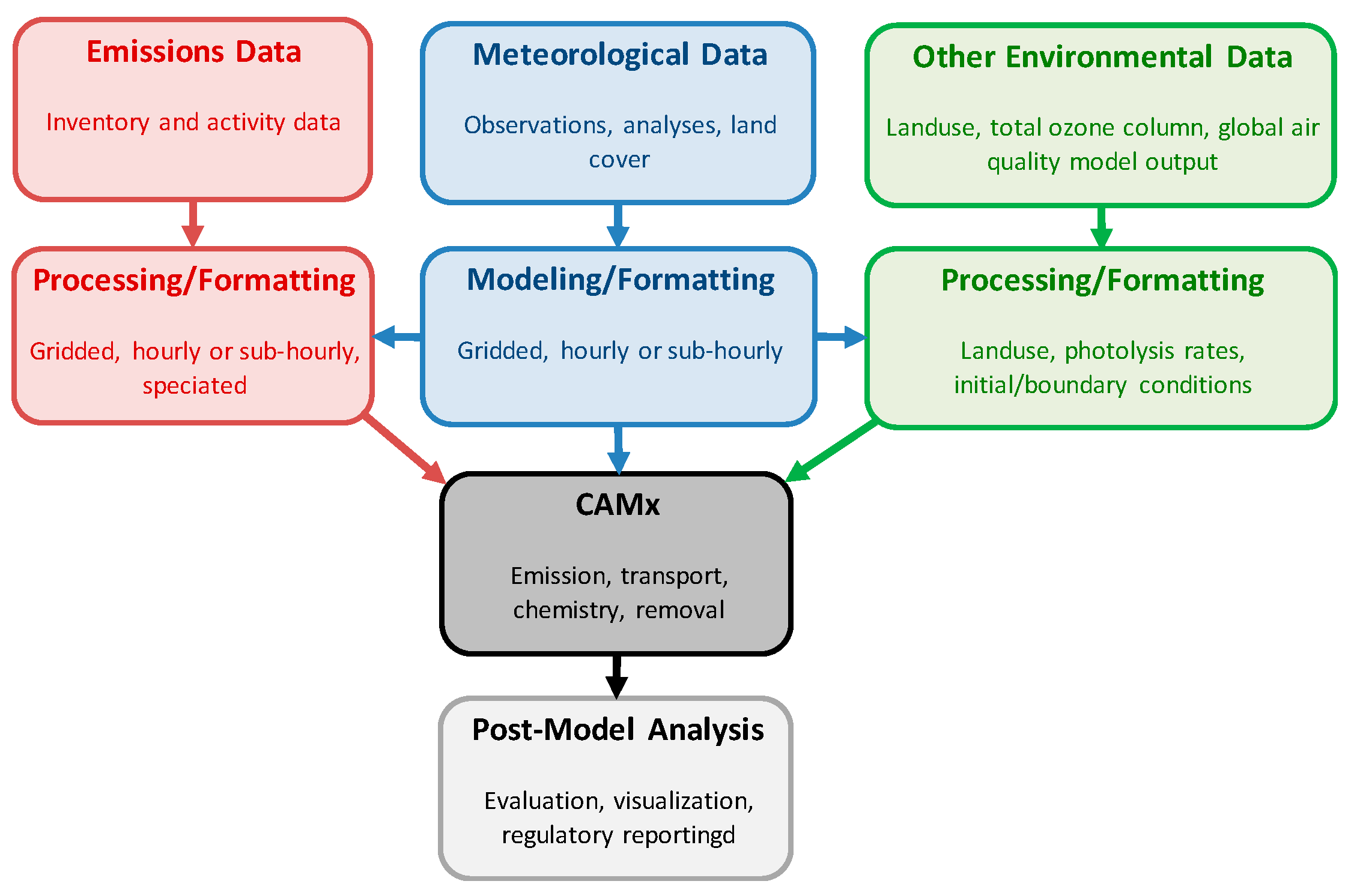
Figure 1. Schematic diagram of the CAMx modeling system.
Atmosphere 15 01158 g001
Figure 2. Schematic of surface deposition and emission pathways showing applicable resistances (R) following an electric circuit analog. The left side shows the standard Zhang unidirectional deposition scheme [21]; the right side shows the Zhang bidirectional NH3 scheme [28,50] with NH3 compensation points (C).
Atmosphere 15 01158 g002
Figure 3. Schematic of CiG within a single CAMx multi-layer grid column (outer box), indicating CiG cloud volume (cylinder), area coverage (fc), ambient and in-cloud vertical fluxes (Fa, Fc), and entrainment/detrainment fluxes (E, D). Vertical layer depth and indexing are noted with dz and k.
Atmosphere 15 01158 g003
Figure 4. Schematic diagram of the SOAP scheme for modeling interactions between anthropogenic organic emissions and SOA formation in CAMx. A similar process is applied for biogenic VOCs without POA or IVOA pathways.
Atmosphere 15 01158 g004
Figure 5. Schematic diagram of the CAMx 1.5-D VBS module. Species name consists of four characters that indicate the phase (P—particle; V—vapor), the source (A—anthropogenic; B—biogenic; C—cooking; F—fire), the formation (P—primary; S—secondary), and the volatility bin number. The solid and dashed black arrows represent gas–aerosol partitioning and chemical aging, respectively. The thick, colored arrows represent POA emissions or the oxidation of SOA precursors.
Atmosphere 15 01158 g005
Figure 6. Modeling domains for the EPA 2016 modeling platform, each noting their respective grid spacing [10].
Atmosphere 15 01158 g006
Figure 7. Locations of AQS/AIRS ozone monitoring sites used for model performance evaluation.
Atmosphere 15 01158 g007
Figure 8. Locations of CSN and IMPROVE PM monitoring sites used for model performance evaluation.
Atmosphere 15 01158 g008
Figure 9. Locations of CASTNET PM and AMON ammonia monitoring sites used for model performance evaluation.
Atmosphere 15 01158 g009
Figure 10. Nine NOAA climate regions used for model performance evaluation.
Atmosphere 15 01158 g010
Figure 11. Monthly comparison between the 2016 observed (gray) and simulated (blue) MDA8 ozone concentrations for each of the nine NOAA climate regions shown in Figure 10. Boxes represent the interquartile range (25th to 75th percentile with median shown by the center line), dashed whiskers represent 1.5 times the interquartile range, and circles represent individual outlier values.
Atmosphere 15 01158 g011aAtmosphere 15 01158 g011b
Figure 12. Statistical model performance (NMB, NME, r) in replicating MDA8 ozone over the April–September 2016 season by US climate zone. Criteria benchmarks are shown as red lines.
Atmosphere 15 01158 g012
Figure 13. Monthly comparison between the 2016 observed (gray) and simulated (blue) 24 h total PM2.5 concentrations for each of the nine NOAA climate regions shown in Figure 10. Boxes represent the interquartile range (25th to 75th percentile with median shown by the center line), dashed whiskers represent 1.5 times the interquartile range, and circles represent individual outlier values.
Atmosphere 15 01158 g013aAtmosphere 15 01158 g013b
Figure 14. Statistical model performance (NMB, NME, r) in replicating 24 h total PM2.5 over the April–September 2016 warm season by US climate zone. Criteria benchmarks are shown as red lines.
Atmosphere 15 01158 g014
Figure 15. Statistical model performance (NMB, NME, r) in replicating 24 h total PM2.5 over the combined January–March and October–December 2016 cool seasons by US climate zone. Criteria benchmarks are shown as red lines.
Atmosphere 15 01158 g015
Figure 16. Observed April–September average ammonia concentrations (ppb) at AMON sites (top) and simulated ammonia mean bias (MB, ppb) with the bidirectional scheme (lower left) and without the bidirectional scheme (bottom right).
Atmosphere 15 01158 g016
Figure 17. Observed October–March average ammonia concentrations (ppb) at AMON sites (top) and simulated ammonia mean bias (MB, ppb) with the bidirectional scheme (lower left) and without the bidirectional scheme (bottom right).
Atmosphere 15 01158 g017
Table 1. Summary of CAMx numerical treatments and solver methods for key processes.
ProcessNumerical TreatmentSolver Methods
Horizontal advectionFinite difference flux divergencePiecewise Parabolic Method (PPM) [19,20]
Non-linear renormalized integrated flux [21]
Vertical advectionFinite difference flux divergencePPM [19,20]
Implicit backward Euler (time) centered (space) [22]
Horizontal diffusionFinite difference K-theoryExplicit simultaneous 2D solver
Vertical diffusionFinite difference K-theory
Non-local asymmetric mixing
Implicit backward Euler (time) centered (space) [22]
Asymmetric Convective Model, v2 (ACM2) [23]
Dry depositionResistance models for gasses [24,25]
Resistance models for aerosols [26,27]
Bi-directional ammonia flux [28]
Deposition velocity as surface boundary condition for vertical diffusion
Sub-grid cloud convectionEntraining/detraining plume model [29]
Wet depositionScavenging model for gasses and aerosols [1]
Gas chemistryCarbon Bond v6 (CB6) [30,31,32,33,34,35]
Statewide Air Pollution Research Center 2007 (SAPRC07) [36,37]
Euler Backward Iterative (EBI) [38]
Livermore Solver for Ordinary Differential Equations (LSODE) [39]
Inorganic aerosol chemistryISORROPIA [40,41]
Equilibrium Simplified Aerosol Model (EQSAM) [42]
Aqueous aerosol chemistryRegional Acid Deposition Model (RADM-AQ) [43]
Organic aerosol chemistrySOAP [44]
1.5-D Volatility Basis Set (VBS) [45]
Table 2. Gas-phase chemical mechanisms implemented in CAMx v7.20.
MechanismDescription
CB6r2hCarbon Bond v6, Revision 2 [30,31,34] extended to include a full suite of oceanic halogen chemistry [32].
304 reactions among 115 species.
CB6r4Carbon Bond v6, Revision 4 adds temperature- and pressure-dependent NO2-organic nitrate branching [35], a condensed oceanic iodine mechanism in lieu of full halogen chemistry, and oceanic dimethyl sulfide reactions.
233 reactions among 86 species.
CB6r5Carbon Bond v6, Revision 5 [33] adds updated chemical reaction data for inorganic and simple organic species.
234 reactions among 86 species.
SAPRC07TCThe Statewide Air Pollution Research Center 2007 mechanism supporting toxics [36,37].
565 reactions among 117 species
Table 3. SOAP species, associated VOC precursors, and chemistry parameters.
SpeciesVOC PrecursorsAerosol Mass Yield 1Saturation Concentration (
C*) [µg/m3] at 300 K
Volatility
ΔHvap [kJ/mol]
Molecular Weight [g/mol]
SOA1/CG1Benzene0.487/0.24814116150
Toluene0.663/0.304
Xylene0.291/0.084
IVOA0/0.012
SOA2/CG2Benzene0.167/0.3910.31147150
Toluene0.345/0.293
Xylene0.306/0.049
IVOA0.275/0.225
SOPABenzene0/00-220
Toluene0.262/0.044
Xylene0.294/0.025
IVOA0.277/0.129
SOA3/CG3Isoprene0.156/0.07626118180
Monoterpene0.150/0.075
Sesquiterpene0.136/0.092
SOA4/CG4Isoprene0.029/0.0230.45123180
Monoterpene0.090/0.045
Sesquiterpene0.400/0.328
SOPBIsoprene0.011/00-220
Monoterpene0.070/0.070
Sesquiterpene0.270/0.175
1 Mass-based yields of CG products from VOC precursors (low-NOx yield/high-NOx yield).
Table 4. CAMx v7.20 model configuration for the 2016 application.
OptionSetting
Horizontal advectionPPM
Vertical advectionPPM
Gas chemistry mechanismCB6r5
Gas chemistry solverEBI
PM chemistryCF with explicit elements
Probing ToolsOff
Dry depositionZhang
Bidirectional ammoniaOn and Off
ACM2 vertical diffusionOn
Sub-grid cloud convectionOff
In-line oceanic iodine emissionsOn
Table 5. Model statistical performance criteria proposed by Emery et al. [110]. Criteria for NO3, OC, and EC correlation were not proposed due to large statistical uncertainty.
PollutantNMBNMEr
MDA8 Ozone<±15%<25%>0.50
24 h total PM2.5, SO4, NH4<±30%<50%>0.40
24 h NO3<±65%<115%--
24 h OC<±50%<65%--
24 h EC<±40%<75%--
Disclaimer/Publisher’s Note: The statements, opinions and data contained in all publications are solely those of the individual author(s) and contributor(s) and not of MDPI and/or the editor(s). MDPI and/or the editor(s) disclaim responsibility for any injury to people or property resulting from any ideas, methods, instructions or products referred to in the content.