Abstract
A first-order linear and numerically non-diffusive Eulerian transport algorithm, minVAR, was recently developed for preservation of correlations between interrelated tracers during advective transport. The present study extends this work by: (1) providing further investigation of several interesting geometric constructions found in contours of constant minVAR, short for minimum variance, through extension to three coordinate dimensions. These contours capture point-by-point representations of thousands of individual atmospheric aerosol and/or cloud particles as they evolve and are rendered on Eulerian grids at a level of sub-grid resolution limited only by numerical precision; and (2) exploration of geometric similarities between the Arakawa C-grid, used to obtain interpolated values of the wind field at grid scale and minVAR. In particular, we consider interpolation of the u and v horizontal components of wind velocity from grid to sub-grid scales. The last results are motivated by recent applications of the Weather Research and Forecasting (WRF) model applied in the coastal Houston region, where the recent TRacking Aerosol Convection Interactions ExpeRiment (TRACER) field campaign was organized. A unique and fully consistent mapping is obtained between particles moving along meteorological wind trajectories and the non-diffusive, non-dispersive representation of such trajectories on an Eulerian grid.
1. Introduction
The spatial transport of atmospheric particles and coupled chemical species has long been a challenge using higher-order advection schemes [1,2,3,4,5], while first-order linear schemes are rarely (if ever) used by the atmospheric modeling community due to their considerable numerical diffusion. Lauritzen and Thuburn give a powerful statement of the problem in [4]: “We are not aware of any transport scheme that is both shape-preserving on individual tracers and sum-preserving for three or more tracers, and, indeed, it is not clear whether such a scheme is possible.” A new approach, minVAR (short for minimum variance), recently developed in [1], appears to go a long way in eliminating many of the problems associated with higher-order transport schemes, in so doing minVAR retains all the positive features of a first-order linear scheme (it is one) while being completely non-diffusive. Moreover, minVAR has been demonstrated to actually achieve sum and shape preservation for three tracers as shown in [1].
We show critical geometric features produced by contours of constant minVAR that are important to the new method. These features are illustrated here for 2- and 3-dimensional grids and found to exhibit symmetries that are related here to the most basic and important properties of minVAR, namely, that the algorithm is both linear and numerically non-diffusive (Section 1 below and Section 2). This combination of properties appears to be unique to the new advection scheme. Linearity makes it possible to preserve correlations between interrelated tracer sets, while facilitating great computational speed. Non-diffusivity enables the tracking of tracers (e.g., air pollutants) with unprecedented levels of spatial and temporal resolution limited only by numerical precision. The last feature is demonstrated here using WRF model output and verified through comparison with field campaign observations (Section 3).
The minVAR algorithm is linear and thus satisfies a superposition principle that connects these geometric features across dimensionality with extension from one to two and three coordinates. This section reviews the one-dimensional case. Section 2 presents new findings found in extensions of the algorithm to two and three coordinates. Section 3 discusses certain structural similarities with minVAR that were discovered in simulations performed with the WRF model on an Arakawa-C grid [6]. Section 4 gives a summary and discussion of future directions.
Figure 1 illustrates several key features of minVAR as applied the simplest case of 1-D advective transport in a uniform horizontal wind field. Colors in the left panel represent tracer mass initially (step 0), where a unit of conserved tracer is introduced uniformly throughout grid cell 0. Time evolution of tracer follows a series of advection steps, advancing to the right under a constant Courant number where u is windspeed in the positive x direction, is cell width and is the time step. Each of these quantities is assumed to be uniform for purpose of illustration. A pulse initially located at the origin will be centered at the product of k and c after the kth advection step. After the 20th step the pulse will be centered on grid cell 3 (equal to 20 × 0.15) to form a perfectly shifted recurrence of the initial condition as expected in the absence of numerical diffusion. The algorithm is absolutely stable, as the pattern of recurrence repeats indefinitely in multiples of 20 steps and is reversible with change in wind direction. Residual spread in the distribution is seen in the figure at non-multiples of 20 steps. This spread, which is maximal after 10 steps, derives from the mathematical representation of a zero-dimensional point, moving with the center of mass of the advecting tracer pulse, across the finite-width cells of the Eulerian grid.
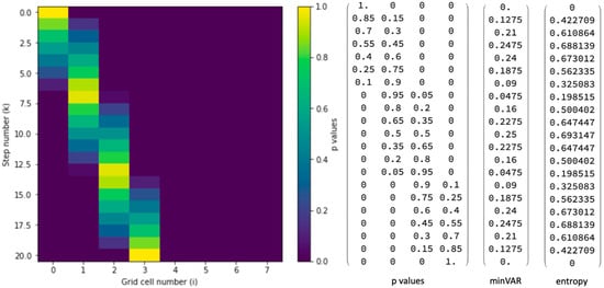
Figure 1.
Color-shaded representation of a unit tracer pulse undergoing advection on a uniform one-dimensional grid. Cell occupation numbers (p-values), here normalized to unity, give the total amount of conserved tracer material within each grid cell. These are illustrated graphically according to the color scale, with numerical values given by the corresponding matrix rows appearing to the right. Note that the four rightmost columns (4–7) containing zeros were cut to save space. The rightmost vectors give two distinct metrics, minVAR and entropy, for assessing spread in the p-value distributions. As points have dimension zero, such spread is a mathematical effect associated with the mapping of Lagrangian points (tracer centers of mass) to the Eulerian grid, using functions described in Table 1, Table 2 and Table 3.
Two distinct approaches were developed in paper [1] for obtaining the minVAR and p-values given in Figure 1. The first, and most easily generalizable approach is based on linear programming (LP). For LP, variance serves as the cost function, which is to be minimized subject to two equality constraints: (1) preservation of x-coordinate position for the Lagrangian point being represented (y and z coordinates are recovered similarly using their values, in place of x, in the argument list of the program), and (2) conservation of total tracer amount (sum of p-values) here normalized to unity. Finally, a set of inequality constraints ensures positivity of the p-values, for all i. LP offers several advantages over minVAR: (1) it is more intuitive with an instruction set reading like the sentences of an open book (Table 1), (2) as it minimizes the cost function to obtain minVAR, the p-values are computed automatically. (3) LP is more easily generalizable to stationary non-uniform grids. On the other hand, for uniform grids minVAR is much faster to compute. Table 1 shows the one-dimensional case, LP1D. The corresponding case for minVAR (mV1D) is given in Table 2 together with extensions to two and three dimensions. The computation of p-values is described in Table 3 for completeness following the cell numbering convention introduced in [1]. For the remainder of this paper, we will need only the minVAR values themselves. These are available from the simple analytic expressions given in Table 2. Each of these tables contains editable code that is executable in Mathematica [7].

Table 1.
Linear Program for one-dimensional grids of length n + 1: . is the occupation fraction of normalized material in grid cell i centered at . The case n = 7 (eight cells) was used to generate the color-shaded representation, occupation numbers, and minimum variance (minVAR) values of Figure 1. Chop[expr] replaces approximate real numbers in expr that are close to zero by the exact integer 0.

Table 2.
Analytic functions used to compute minVAR values in 1–3 coordinate dimensions. Floor[x] gives the greatest integer less than or equal to x.

Table 3.
Analytic functions used to compute p-values in 1–3 coordinate dimensions using back projection via the outer product in 2 and 3 dimensions. Note that the function mV1D from Table 2 is required to initiate the process. p1D, p2D, and p3D generate 3, 9 and 27 cell entries following the cell numbering given in [1]. Chop[expr] replaces approximate real numbers in expr that are close to zero by the exact integer 0.
2. Extensions of the Algorithm to Two- and Three-Dimensional Grids
Table 2 lists three relatively simple analytic functions for computing the minimum variance (minVAR) representation of individual Lagrangian points represented on Eulerian grids in 1, 2, and 3 dimensions. The lines of code are Mathematica executable as they appear. Further explanation and illustration of the working of these formulae is provided in the Appendix A.
Figure 2a shows contours of constant minVAR within a unit grid cell. This pattern is periodic, repeating from cell-to-cell across the grid. Contours from cell center to corners are (0.01, 0.05, 0.10, 0.15, 0.20, 0.25 (boundary of the yellow-shaded region), 0.30, 0.35, 0.40, 0.45, and 0.499) the first and last entries mark the near center and near corner positions, respectively. Central slices along x = 1 and y = 1 give contour values spanning the range of minVAR in 1D, from 0 to 0.25 (cf. Figure 1). For the 2D case the range is from zero, at the center, to 0.5 at the corners. minVAR values of 0.25 in 2D lie at the four sharp astrid tips located at the centers of the grid’s square (more generally rectangular) boundaries and along the astrid itself. The points at a tip map to tracer mass being evenly distributed between the illustrated cell and its neighboring cell on the grid. A point at one of the four corners has the largest minVAR value of 0.5, as that point is shared by four cells including the illustrated cell and three closest neighbors, which three depends on which corner is involved, as determined by the Floor function of Table 2. Its rendering on the Eulerian grid is described by these same four unit squares equally sharing tracer mass with p-values of 1/4 each.
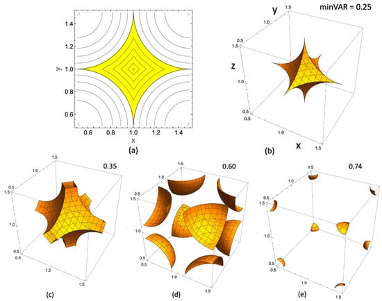
Figure 2.
minVAR contour plots in two (a) and three-coordinate dimensions (b–e). For the surfaces in three dimensions, the minVAR values are shown above each figure, ranging from 0.25 to close to the 3D maximum value of 0.75 from Table 2. Disposition of the x, y, and z coordinates is shown in (b).
Figure 2b shows a full astrid surface in 3D with its six sharp tips centered on the six sides of the cube. For these tips the minVAR value is 0.25 as tracer mass is once again shared, here by two neighboring cubes, the one illustrated and its neighbor on the grid. Of course, the entire astrid surface, being a contour, has this same minVAR value. A point at one of the eight cube corners has the largest minVAR, equal to 0.75, and represents tracer material shared equally among the illustrated cube and its seven neighbors, each with a p-value of 1/8.
To summarize, the maximum minVAR values in 1, 2, and 3 dimensions are 1/4, 1/2, and 3/4. These are the same integer ratios that appear prominently in the analytic functions of corresponding dimensionality in Table 2. In all cases, the p-values sum to unity as expected given that tracer normalization is preserved both in minVAR and in LP.
Entropy and minVAR are each maximized when the tracer is evenly spread over a maximal number of grid cells, restricted to eliminate numerical diffusion. As shown above, the restricted number of cells is 2d, where d is dimensionality of the grid. The case for d = 1 (2 cells) is easily found to follow the ratio:
by ratioing the largest elements from the entropy and minVAR columns of Figure 1. Here, we show that this ratio, used as a scaling factor to match peak heights in Figure 3, is invariant to dimensionality of the underlying grid.
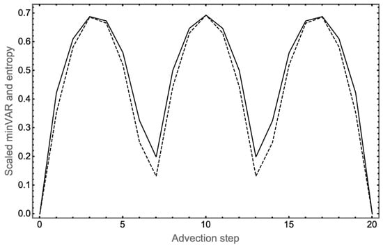
Figure 3.
Comparison of minVAR and entropy as metrics of tracer spread: Solid curve, distributional entropy as a function of the number of completed advection steps. Dashed curve, minVAR values scaled by the factor 4 ln(2) = 2.77259 so as to match the peak value of the entropy for a clearer comparison of the two metrics. Numerical values are listed in the rightmost columns of Figure 1. Interestingly, this scaling factor is unchanged going from one to two- and three-dimensional grids (see below).
It was shown above that max minVAR = d/4 for grid dimensionality d. The max entropy of a discrete distribution takes the form [8]:
where the entropy, S, has been non-dimensionalized on dividing by the Boltzmann constant k (erg/deg). The final equality follows from the max entropy condition achieved when each of the p-values takes the value 1/2d as shown above. Dividing Equation (2) by max minVAR = d/4 leads to cancellation of dimensionality and recovery of Equation (1).
3. Exploiting Similarities with the Arakawa-C Grid Using WRF
The Weather Research and Forecasting Model (WRF) employs the Arakawa C-grid with terrain-following pressure-based sigma, for its numerical simulations [9,10]. The WRF model calculates u (east–west) and v (north–south) wind components by solving the horizontal momentum equations, which include forces such as Coriolis effects, friction, and pressure gradients. On a staggered grid, the model integrates these equations over time. The Arakawa grid system is a method of discretizing the atmosphere for numerical weather prediction and climate models, with the C-grid being one of several possible configurations. In the C-grid arrangement, east–west (u) and north–south (v) velocity components are staggered with respect to scalar variables like the mass of chemical species concentrations. This configuration allows WRF to achieve more accurate and stable simulations of atmospheric dynamics and chemical processes, which are crucial for understanding and predicting weather patterns, air quality, and the dispersion of pollutants. Initial and boundary conditions are provided by external datasets (e.g., North American Mesoscale Forecast System (NAM) datasets available at https://www.ncei.noaa.gov/, accessed on 2 October 2022), while physical processes like turbulence and convection are parameterized to refine the wind calculations. These components evolve within the model’s framework to produce detailed wind fields, which are later converted to wind speed and direction for analysis.
The US Department of Energy (DOE)-Atmospheric Radiation Measurement’s (ARM) TRacking Aerosol Convection Interactions ExpeRiment (TRACER) field campaign, conducted from 1 October 2021, to 30 September 2022, along with intensive summertime observations at additional rural and urban locations in southern Texas, offered a unique opportunity to study aerosol processes in Houston’s distinctive urban and coastal environment [11]. In this study, we employ the WRF model to simulate the wind velocities over the coastal region of Houston.
Figure 4 shows a true color image obtained using the NOAA-20 Visible Infrared Imaging Radiometer Suite (VIIRS) [12], illustrating the domain centered at La Porte (the Main observation site) and bounded by 27 to 32° N and -97 to −93° E. The model simulations were conducted from 1 July to 30 August 2022, at 5 × 5 km horizontal resolution with 45 vertical layers. The model configuration details are provided in Table 4. The simulation result on 20 July 2022 is used for this study. The figure also includes an example of the modeled u and v velocity components over the Arakawa C-grid (domain a). The u components are at the centers of the left and right grid faces, and the v components are at the centers of the upper and lower grid faces. Further analysis is carried out using these model outputs from domain b.
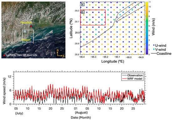
Figure 4.
True color image obtained using NOAA-20 Visible Infrared Imaging Radiometer Suite (VIIRS) on 20 July 2022 (left panel). The red triangle marks the main site of observation (La Porte) during the TRACER field campaign. The white box encloses domain a, where WRF-modeled u, and v wind velocities are shown (right panel) on 20 July 2022 at 00 UTC. The red box encloses domain b, used for the analysis in Figure 5 and Figure 6. Time series of hourly wind speed at 10 m at TRACER main site obtained from observation (black) and WRF model simulation (red) from 4 July to 30 August 2022 is shown in the bottom panel.

Table 4.
WRF model configuration.
These WRF-simulated u and v wind components are used to calculate wind speed, which is then compared with measurements taken during the TRACER field campaign. Figure 4 shows the DOE ARM main site of the TRACER field campaign, located at the La Porte site in southern Texas. These datasets are available at https://adc.arm.gov/discovery (accessed on 2 October 2022). The model overestimates the measured wind speed by approximately 2 m/s (~25%) during the cooler time of the day (~02:00 to 09:00 UTC). For the remainder of the day, the simulated values align well with the measurements. Despite these discrepancies, the modeled values capture the temporal and spatial variation in wind speed and retain the diurnal pattern (Figure 4 bottom panel). Comparable wind biases were observed in earlier WRF model related studies [20,21,22], particularly at lower wind speeds and in areas with greater variability in wind direction. The model domain extending over the southern Texas region helps in understanding some of the regional meteorological phenomena, such as the Sea Breeze phenomenon, which is common over the coastal region.
The red points in Figure 6a,b mark the distribution of 15 u points and 16 v points from the domain b in Figure 4 and enlarged in Figure 5. These points are crucial for the interpolation process, lying on the interpolation surface, which facilitates the transition from discrete data points to a continuous field. This interpolation is necessary to accurately capture the variations in wind components across the grid. The figure also showcases the resultant interpolated wind vectors, which are computed using the interpolated u and v fields. This detailed interpolation in the sub-grid scale is essential for improving the precision of weather models by providing a more refined and continuous representation of wind patterns.
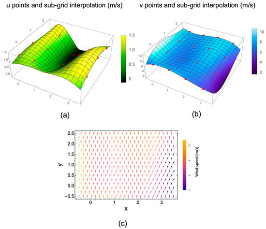
Figure 6.
(a) u points (red) from Figure 4 (green in Figure 5) and sub-grid interpolation, (b) v points (red) from Figure 4 (blue in Figure 5) and sub-grid interpolation, (c) interpolated wind vectors having components given by the u and v fields, (a,b), respectively. Color scales in m/s. See Figure 5 for mapping between latitude/longitude values and Cartesian grid coordinates.
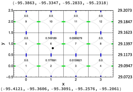
Figure 5.
Alignment of latitude-longitude and Cartesian coordinates on the grid. The figure shows cell numbering and periodicity, encoding of a test point (small black circle), which when represented on the grid using minVAR gives the normalized weights (p-values) shown in the figure. Coordinates of the point are recovered as the center of mass of these weights encoded on the grid. The figure also shows the locations of the u (green), and v (blue) velocity components computed by WRF. These are used to obtain the interpolated sub-grid wind field shown in Figure 6. The astrids each correspond to the boundary of the yellow-shaded region (minVAR = 0.25) of Figure 2a. These are joined here to reflect the symmetry of the grid.
4. Summary
It seems remarkable that all the geometric constructions of Figure 2 follow from the comparatively simple functions of Table 2, which on inspection seem largely based on the Pythagorean theorem. Moreover, it is not at all clear how these functions arise in connection with the advection problem. As mentioned, they were only found on inspection of contour plots produced by the linear program, which itself was intended for use only as a limiter for the generally unacceptable levels of numerical diffusion encountered with the basic first-order advection scheme—especially on coarse grids—without, of course, destroying the first-order linear properties of the basic scheme. Moreover, both methods, minVAR and LP, give identical results for the case comparisons to which they have been subjected, and both totally eliminate numerical diffusion as shown by reversibility and, for rational Courant numbers, perfect recovery of the (albeit shifted) initial condition as shown in Figure 1.
Entropy has been used as a metric for the extent of numerical diffusion in model testing, and Figure 3 makes a scaled comparison with minVAR for this purpose. The logarithm in entropy ensures its additivity for independent systems in statistical applications but has disadvantages for use as a metric of fidelity preservation in advective transport models. First, the logarithm is non-linear and, as such, does not serve well as a cost function to a linear program–based advection scheme intended to preserve first-order linearity. Second, there is no sensitivity to grid position in the entropy function whereas minVAR and LP both include grid coordinates in their definition of the cost function. These are common concerns working with entropy in this and other applications. One solution, suggested by inspection of similarities between the two curves of Figure 3, is to simply use the scaled minVAR function, in place of entropy when a linear cost function is required.
The Arakawa C-grid has been combined with minVAR to perform sub-grid scale interpolation of the wind fields from the WRF model. This technique is demonstrated for a 15 by 20 km2 area in the Houston coastal region during the modeled period of TRACER field campaign. This example can be used to enhance the accuracy of weather models, as it provides a more refined and continuous depiction of wind patterns. As an example, the test point located in cell 6 of Figure 5 having Cartesian coordinates {x, y} = {1.07292, 0.808117} has the interpolated wind components {u, v} = {0.336495, 7.17384}. It also has a unique minimum variance representation given by the weights in cells 2, 3, 6, 7 that precisely encode its position on the Eulerian grid. Linear superposition inherent in either of the two equivalent non-diffusive advection schemes (LP and minVAR) can be used to efficiently represent thousands of such points this way as shown in [1]. As these points disperse across the grid both physical and mathematical (minVAR) variances change. These too can be separated using the linear superposition principle as shown in [1]. Such pointillistic swarms can represent collections of aerosol particles and/or cloud droplets that can now be tracked with almost unlimited precision as they move across the grid. Information on the particle distributions can also be encoded using far fewer optimized quadrature points, super particles, and/or super drops for extra computational speed. Similar considerations might also apply to the optimized deployment of sensor networks. Key findings include: (1) Particle coordinates of atmospheric aerosols and clouds are rendered with high precision and computational efficiency on Eulerian grids in one, two, and three coordinate dimensions. (2) These renderings exhibit interesting geometric features that are the focus of the present study. (3) Notable structural similarities between minVAR and the Arakawa C-grid structure used in the Weather Research and Forecasting (WRF) model are shown to enable more precise interpolation and finer spatial resolution of wind fields, facilitating enhanced model accuracy that can be applied to better understand localized atmospheric phenomena.
Author Contributions
R.M. is responsible for results described in Section 2 and the Appendix A; T.S. is responsible for results described in Section 3; Both authors contributed equally to development of Section 1 and Section 4. All authors have read and agreed to the published version of the manuscript.
Funding
This research was funded by the U.S. Department of Energy under Grant DE-SC0012704.
Institutional Review Board Statement
Not applicable.
Informed Consent Statement
Not applicable.
Data Availability Statement
Acknowledgments
R. McGraw (BNL) and T. Subba (BNL) acknowledge the Atmospheric Systems Research (ASR) Program of the U.S. Department of Energy (Grant DE-SC0012704) for financial support. We also would like to acknowledge support from the Atmospheric Radiation Measurement (ARM) user facility, and the ARM TRACER operation and science teams. This research used resources of the National Energy Research Scientific Computing Center, a DOE Office of Science User Facility supported by the Office of Science of the U.S. Department of Energy under Contract No. DE-AC02-05CH11231 using NERSC award BER-ERCAP0026649. In addition, the NE Linux Cluster (nlc) at Brookhaven National Laboratory was utilized for model simulations and data storage.
Conflicts of Interest
The authors declare no conflict of interest.
Appendix A. Rendering Points on a Large Eulerian Grid Using minVAR
Appendix A1. minVAR Values from Table 2
Consider an arbitrary point in 3D, its coordinates, and the minimum possible variance (minVAR) associated with its Eulerian representation on grids in 1, 2, and 3 dimensions. Let the point in three dimensions have coordinates {x, y, z} = {4.75, 1.23, 0.71}. Its minVAR values (coordinate-by-coordinate) are {mV1D[x], mV1D[y], mV1D[z]} = {0.1875, 0.1771, 0.2059}
Testing the functions of Table 2 gives expected results for back projection of 1D projections to obtain results in 2 and 3 dimensions:
{mV1D[x] + mV1D[y], mV2D[{x, y}]} = {0.3646, 0.3646}.
{mV1D[x] + mV1D[y] + mV1D[z], mV3D[{x, y, z}]} = {0.5705, 0.5705}.
Other identities are consistent with the central slice theorem of tomography:
{mV2D[{x, 1}] + mV2D[{1, y}], mV2D[{x, y}]} = {0.3646, 0.3646}.
{mV3D[{x, 1, 1}] + mV3D[{1, y, 1}] + mV3D[{1, 1, z}], mV3D[{x, y, z}]} = {0.5705, 0.5705}.
{mV3D[{4.75, 1.23, 0.71}], mV1D [4.75] + mV1D [1.23] + mV1D [0.71]} = {0.5705, 0.5705}.
Additional notes: The central slice theorem relates the 1-D Fourier transform of a projection with the 2 D Fourier transform of the region of the image from which the projection was obtained. Here, for example, projections along the x and y axes generate the 2D Eulerian representation of a point in 2D, while projections along the x, y, and z axes generate the 3D Eulerian representation of a point in 3D. As tracer composition is uniform within each grid cell, the Eulerian representation of a point is, in effect, pixelated, and the discrete cosine transform (DCT) of image processing could be used instead, but even this is unnecessary as the functions presented in Table 3 do this automatically for an Eulerian grid.
Appendix A2. p-Values from Table 3
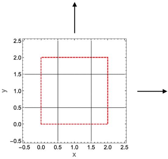
Figure A1.
Position of the reference plaquette located near the grid origin in two dimensions. Arrows are a reminder that the reference plaquette is part of a much larger grid. Only points within or on the dashed red square can be rendered on this small Eulerian grid of nine cells (c.f. Figure 6 of [1]). Cells 1-9 are numbered according to the convention of increasing going from left to right (increasing x) and from bottom to top (increasing y). Thus, the lower row cells are numbered 1, 2, 3 going left to right, and the upper row 7, 8, 9 going in the same direction.
Of course, individual points and collections of points need to be rendered anywhere on the extended grid. Those outside of the red square can be rendered either by moving the plaquette (similar to the way a stencil is moved across the grid when doing finite differencing) or the coordinates of distant points can be shifted so as to fit within or on the red square boundary of the reference plaquette. We choose the latter approach here. Consider the point {x, y} = {4.75, 1.23}, whose x coordinate lies outside the dashed red square. We adapt the following rule:
Shift rule: If the integer part of the x-coordinate of a distant point is even, as in this example, the shifted x value lies between 0 and 1 of the reference plaquette. If it were odd, the shifted x value would lie between 1 and 2. The fractional part is left unchanged. Thus, the shifted point coordinates will always have integer parts even or odd according to whether the original point coordinates were even or odd. This holds also for coordinates y and z in 2 and 3D.
According to the rule, the point {x, y} is shifted to coordinates {0.75, 1.23} suitable for rendering using the reference plaquette. In general, as points move arbitrarily across the grid their shifted image point will travel within the 2x2 red square, with periodic boundary conditions in 1D and toroidal boundary conditions in 2 and 3D.
Reference to the functions of Table 2 shows the identity, {mV1D [0.75], mV1D [4.75]}= {0.1875, 0.1875}, indicating that the minVAR values are identical for the distant and shifted x-coordinate. On the other hand, the p-value functions of Table 3 are suitable only for rendering points within or on the red square of Figure A1, hence the need for the rule and previous discussion. For the nine grid squares of the plaquette:
p2D[{0.75, 1.23}] = {0, 0, 0, 0.1925, 0.5775, 0, 0.0575, 0.1725, 0}.
Applying the same function to the distant point gives instead:
p2D[{4.75, 1.23}] = {0, 0, 0, 4.0425, -10.2025, 6.93, 1.2075, −3.0475, 2.07.
showing unphysical p-values having negative entries according to this naive calculation, despite the fact that minVAR values and normalization to unity are identical to those of the shifted point. The purpose of the rule is to simply assign the same plaquette values (Eulerian representations) to both points. In effect the reference plaquette serves as a scratchpad: distant points are shifted to the red-box region of Figure A1, where calculations are performed to fill the plaquette, thereby obtaining its shifted 3x3 Eulerian representation. The latter is then simply translated in reverse (in this case 4 units to the right) to its natural position. The calculation is simply repeated this way for the potentially thousands of points dispersed across the grid.
The following Mathematica code shifts distant points to the reference grid using the even-rule above:
Shift vector components:
The following functions shift a distant point {x, y} to {xR[x], yR[y]} lying within the red square of the reference plaquette (Figure A1) and computes the vector having even-integer components needed to restore the shifted point back to its original position.
xR[x_] := Mod[IntegerPart[x], 2] + FractionalPart[x].
yR[y_] := Mod[IntegerPart[y], 2] + FractionalPart[y].
zR[z_] := Mod[IntegerPart[z], 2] + FractionalPart[z].
Mod gives the remainder on division of the integer part of x by 2. Note that p-values for the shifted point obtained from Table 3 are subsequently reversed shifted along with the point itself back to its original position {x, y} or {x, y, z). The result is the points {4.75, 1.23} and {0.75, 1.23} now both have the same minVAR and same p-values, and they are related through the even-integer component shift vector Shift2D = {4, 0}:
Shift2D[i_] := {x[i], y[i]} − {xR[x[i]], yR[y[i]]}.
where [i] is the particle index. Adding center coordinates, {1, 1}, of the reference plaquette to the Shift2D[i] coordinates gives the center coordinates labeling the unique plaquette onto which the ith particle, having cartesian coordinates {x, y}, is mapped. In case that multiple points are found occupying the same plaquette, the linear superposition principle is available, as both LP and minVAR are fully linear. As a result of linear superposition, the purely mathematical variances associated with minVAR are easily removed, leaving physical quantities intact, as illustrated for a cloud of 1000 points in [1].
References
- McGraw, R.; Yang, F.; Fierce, L.M. Preserving tracer correlations in moment-based atmospheric transport models. J. Adv. Model. Earth Syst. 2024, 16, e2023MS003621. [Google Scholar] [CrossRef]
- Wright, D.L. Numerical advection of moments of the particle size distribution in Eulerian models. J. Aerosol Sci. 2007, 38, 352–369. [Google Scholar] [CrossRef]
- Ovtchinnikov, M.; Easter, R.C. Nonlinear advection algorithms applied to interrelated tracers: Errors and implications for modeling aerosol–cloud interactions. Mon. Weather Rev. 2009, 137, 632–644. [Google Scholar] [CrossRef]
- Lauritzen, P.H.; Thuburn, J. Evaluating advection/transport schemes using interrelated tracers, scatterplots and numerical mixing diagnostics. Q. J. R. Meteorol. Soc. 2012, 138, 906–918. [Google Scholar] [CrossRef]
- McGraw, R. Correcting transport errors during advection of aerosol and cloud particle moment sequences in Eulerian models. In Climate Models; Druyan, L.M., Ed.; InTech Open: London, UK, 2012; Chapter 13; pp. 297–310. [Google Scholar]
- Lundquist, K.A.; Chow, F.K.; Lundquis, J.K. An Immersed Boundary Method for the Weather Research and Forecasting Model. Mon. Weather Rev. 2009, 138, 796–817. [Google Scholar] [CrossRef]
- McGraw, R. Codes Used in Preservation of Tracer Correlations in Atmospheric Transport Models [Software]. 2023. Available online: https://zenodo.org/doi/10.5281/zenodo.7607751 (accessed on 23 September 2024).
- Wannier, G.H. Statistical Physics; Dover Publications, Inc.: New York, NY, USA, 1966; p. 87. [Google Scholar]
- Grell, G.A.; Peckham, S.E.; Schmitz, R.; McKeen, S.A.; Frost, G.; Skamarock, W.C.; Eder, B. Fully coupled “online” chemistry within the WRF model. Atmos. Environ. 2005, 39, 6957–6975. [Google Scholar] [CrossRef]
- Skamarock, W.C.; Klemp, J.B.; Dudhia, J.; Gill, D.O.; Barker, D.; Duda, M.G.; Huang, X.; Wang, W.; Powers, J.G. NCAR Technical Note NCAR/TN-475+STR. In A Description of the Advanced Research WRF Version 3; National Center for Atmospheric Research: Boulder, CO, USA, 2008; 113p. [Google Scholar]
- Jensen, M.P.; Flynn, J.H.; Judd, L.M.; Kollias, P.; Kuang, C.; Mcfarquhar, G.; Nadkarni, R.; Powers, H.; Sullivan, J. A Succession of Cloud, Precipitation, Aerosol and Air Quality Field Experiments in the Coastal Urban Environment. Bull. Am. Meteorol. Soc. 2022, 103, 103–105. [Google Scholar] [CrossRef]
- EarthData. Visible Infrared Imaging Radiometer Suite (VIIRS). Available online: https://www.earthdata.nasa.gov/learn/find-data/near-real-time/viirs (accessed on 20 May 2024).
- Chou, M.-D.; Suarez, M.J.; Ho, C.-H.; Yan, M.M.-H.; Lee, K.-T. Parameterizations for Cloud Overlapping and Shortwave Single-Scattering Properties for Use in General Circulation and Cloud Ensemble Models. J. Clim. 1998, 11, 202–214. [Google Scholar] [CrossRef]
- Mlawer, E.J.; Taubman, S.J.; Brown, P.D.; Iacono, M.J.; Clough, S.A. Radiative transfer for inhomogeneous atmospheres: RRTM, a validated correlated-k model for the longwave. J. Geophys. Res.-Atmos. 1997, 102, 16663–16682. [Google Scholar] [CrossRef]
- Chen, F.; Dudhia, J. Coupling an advanced land surface-hydrology model with the Penn State-NCAR MM5 modeling system. Part I: Model implementation and sensitivity. Mon. Weather Rev. 2001, 129, 569–585. [Google Scholar] [CrossRef]
- Monin, A.S.; Obukhov, A.M. Basic laws of turbulent mixing in the surface layer of the atmosphere. Contrib. Geophys. Inst. Slovak Acad. Sci. USSR 1954, 151, 163–187. [Google Scholar]
- Hong, S.Y.; Noh, Y.; Dudhia, J. A new vertical diffusion package with an explicit treatment of entrainment processes. Mon. Weather Rev. 2006, 134, 2318–2341. [Google Scholar] [CrossRef]
- Grell, G.A.; Devenyi, D. A generalized approach to parameterizing convection combining ensemble and data assimilation techniques. Geophys. Res. Lett. 2002, 29, 38-1–38-4. [Google Scholar] [CrossRef]
- Morrison, H.; Curry, J.A.; Khvorostyanov, V.I. A new double-moment microphysics parameterization for application in cloud and climate models. Part I: Description. J. Atmos. Sci. 2005, 62, 1665–1677. [Google Scholar] [CrossRef]
- Tuccella, P.; Curci, G.; Visconti, G.; Bessagnet, B.; Menut, L.; Park, R.J. Modeling of gas and aerosol with WRF/Chem over Europe: Evaluation and sensitivity study. J. Geophys. Res. 2012, 117, D03303. [Google Scholar] [CrossRef]
- Solbakken, K.; Birkelund, Y.; Samuelsen, E.M. Evaluation of surface wind using WRF in complex terrain: Atmospheric input data and grid spacing. Environ. Model. Softw. 2021, 145, 105182. [Google Scholar] [CrossRef]
- Subba, T.; Zhang, Y.; Steiner, A.L. Simulating the transport and rupture of pollen in the atmosphere. J. Adv. Model. Earth Syst. 2023, 15, e2022MS003329. [Google Scholar] [CrossRef]
Disclaimer/Publisher’s Note: The statements, opinions and data contained in all publications are solely those of the individual author(s) and contributor(s) and not of MDPI and/or the editor(s). MDPI and/or the editor(s) disclaim responsibility for any injury to people or property resulting from any ideas, methods, instructions or products referred to in the content. |
© 2024 by the authors. Licensee MDPI, Basel, Switzerland. This article is an open access article distributed under the terms and conditions of the Creative Commons Attribution (CC BY) license (https://creativecommons.org/licenses/by/4.0/).