Article

Developing a Chained Simulation Method for Quantifying Cooling Energy in Buildings Affected by the Microclimate of Avenue Trees

Department of Bioenvironmental Systems Engineering, National Taiwan University, Taipei 10617, Taiwan
*
Author to whom correspondence should be addressed.
Atmosphere 2024, 15(10), 1150; https://doi.org/10.3390/atmos15101150
Submission received: 22 August 2024 / Revised: 13 September 2024 / Accepted: 24 September 2024 / Published: 25 September 2024
(This article belongs to the Section Biometeorology and Bioclimatology)

Abstract

:
This paper introduces a methodology aimed at bridging the gap between building energy simulation and urban climate modeling. A coupling method was developed through the Building Control Virtual Test Bed (BCVTB) and applied to a case study in Taipei City, Taiwan, to address the microclimate factors of street trees crucial to cooling energy consumption. The use of the Urban Weather Generator for weather file modification revealed a 0.63 °C average air temperature disparity. The coupling method emphasized the importance of accurate wind speed and convective heat transfer coefficients (CHTCs) on building surfaces in determining cooling energy. The results indicated that elevated CHTC values amplify heat exchange, with higher wind velocities playing a crucial role in heat dissipation. The presence of street trees was found to significantly reduce heat flux penetration, leading to a reduction in building surface temperatures by as much as 9.5% during hot months. The cooling energy was lowered by 16.7% in the BCVTB simulations that included trees compared to those without trees. The EnergyPlus-only simulations underestimated the cooling energy needs by approximately 9.3% during summer months. This research offers valuable insights into the complex interactions between buildings and their environments. The results highlight the importance of trees and shading in mitigating the heat island effect and improving energy-efficient urban planning.

1. Introduction

Buildings significantly influence global final energy consumption and energy-related carbon dioxide emissions [1]. A building’s energy performance is heavily influenced by its surrounding microclimate. For this reason, climatic considerations must be taken into account in urban design [2,3]. Over the past few decades, detailed individual building energy modelling has become an established mode of analysis for building designers [4]. Some conventional building energy simulation (BES) tools developed and widely used include TRNSYS [5], DesignBuilder [6], ESP-r [7], CODYBA [8], and EnergyPlus [9]. BES tools usually employ the use of meteorological data. Since buildings cannot be assumed to be stand-alone in an urban context [10,11,12,13,14], meteorological loads cannot be estimated generically as they are particular for each building [15]. To consider the microclimate in building energy simulation studies, it is imperative to establish a connection between urban climate modeling (UCM) and building energy simulation (BES). This coupling necessitates the linkage of specific variables, notably those related to radiation and convection, such as the convective heat transfer coefficient (CHTC). These variables play a pivotal role in governing the exchange of energy between the external environment and the building’s exterior surfaces, which is critical for accurately assessing the building’s energy performance [16].
Bouyer et al. [10] demonstrated an integration approach by combining the Computational Fluid Dynamics (CFD) software Fluent with SOLENE [17] to obtain detailed thermal fluxes, surface temperatures, and energy consumption. Their study revealed the significant impact of considering reflected solar and longwave irradiance from the urban environment on the heating energy demand. Through a comparative analysis of CFD and BES, they reported a notable 30% increase in the cooling energy demand. Yang et al. [18] presented a detailed approach to microclimate and thermal energy coupling. They employed a coupling platform called the Building Control Virtual Test Bed (BCVTB) [19] to integrate EnergyPlus and ENVI-met. Initially, microclimatic parameters were obtained by ENVI-met simulation. The authors replaced the surface temperatures in EnergyPlus with the calculated mean temperature of all the neighboring surfaces simulated by ENVI-met. The solar radiation fluxes were calculated by EnergyPlus, while the humidity, convective flow, and infiltration were calculated by ENVI-met. Although this approach was methodologically innovative, it had some limitations in quantifying the effects of variables such as outside air temperature, wind speed, and longwave radiation [20]. Despite the limitations in Yang et al.’s model, the approach provided a blueprint for closing the gap between the simulation capabilities of EnergyPlus and ENVI-met using the middleware BCVTB. This coupling mechanism and structure seen in Yang et al.’s study was improved by Ramesh [21]. Ramesh refined the microclimate effect evaluation by coupling the surface-level air temperature and wind speed. These corrected values were used to compute the surface boundary conditions of the model, including the CHTC, radiative linear heat transfer coefficient (RLHTC), and infiltration. While the method underwent validation, its application was restricted to the base-case design. A common advantage in these studies is the utilization of the BCVTB, which, due to its quasi-dynamic nature, offers great computing flexibility. Because it is based on the open-source Ptolemy II software environment, it can be coupled with other programs, including Fluent, TRNSYS, MATLAB, Simulink, and Modelica, among others [22]. More recent applications of co-simulation that relate to microclimate analysis can be observed in [23,24,25].
Based on the identified knowledge gaps and the various methods mentioned for evaluating microclimate effects, this study presents the application of a BES-UCM coupling, using the BCVTB platform to a case study in Taipei, Taiwan. As such, this study has the following aims:
  • Generate a modified weather file using UWG to account for anthropogenic heat and urban environments;
  • Create an EnergyPlus–ENVI-met coupling model using the BCVTB platform for microclimate analysis in building energy simulation;
  • Evaluate the performance of the coupling method by comparing the simulated energy consumption results;
  • Evaluate the impact of street trees on the building’s cooling energy demand.

2. Materials and Methods

The overview of this research method is summarized in Figure 1. This methodology involves three main sections: microclimate simulation, energy simulation, and a coupling strategy that facilitates data exchange between the two.

2.1. Urban Context and Domain

2.1.1. Study Area

The building model is in Taipei, Taiwan (Latitude: 25.1, Longitude: 121.8, altitude: 7 m above sea level). Taiwan has a hot and humid subtropical climate. Over 40% of Taiwan’s national energy consumption is attributed to buildings, and because of its subtropical climate, half of this energy use is dominated by cooling (50%) [26]. These buildings near the streets in urban areas are mostly mixed-use residential and commercial buildings, with ground floors normally used for offices or businesses. These urban areas predominantly comprise compact mid-rise, open mid-rise, and some sparsely built buildings [27]. Huang et al. [26] also points out that the peak summer electricity load in Taiwan sets a new record every year. Previous studies comparing rural and urban areas in Taiwan determined that energy consumption in urban areas was up to 81% higher compared to rural areas [28]. It is crucial investigate how the urban microclimate affects the building energy use and search for solutions to reduce it to counteract the urban heat island (UHI) effect.

2.1.2. Building Model

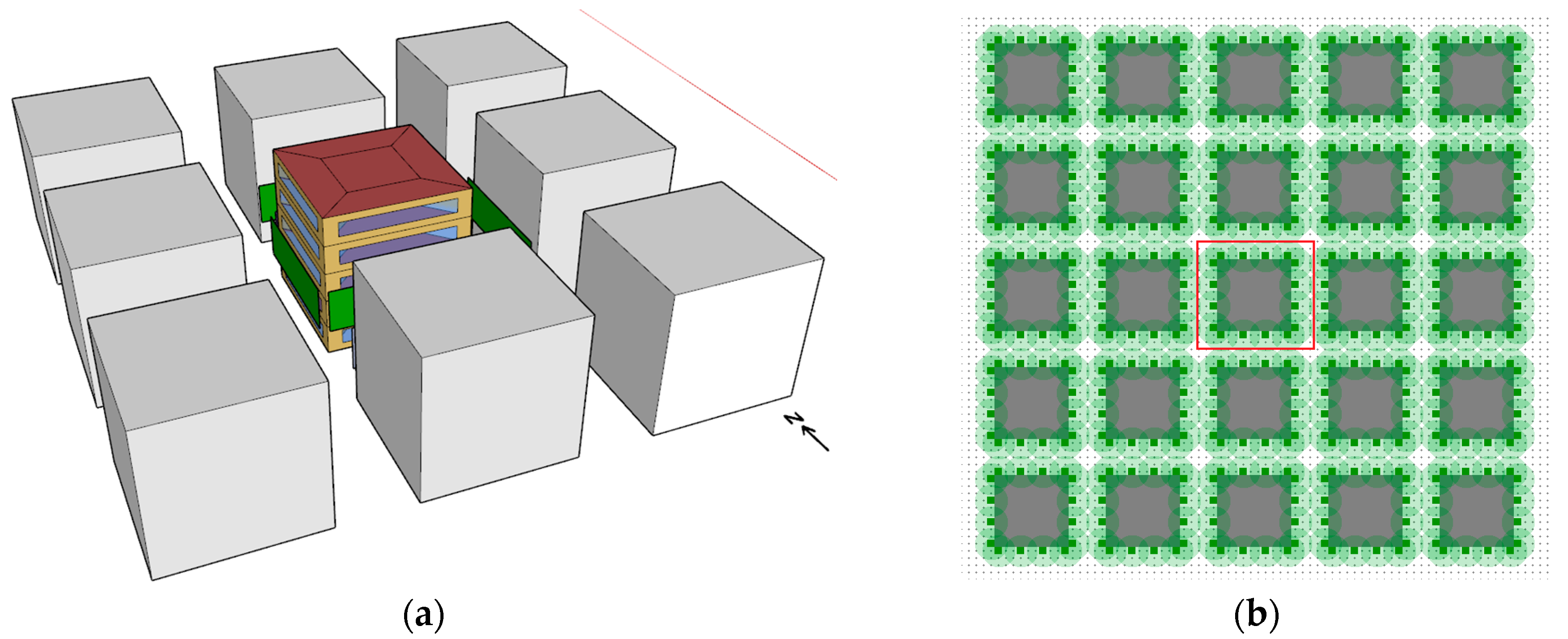
The building model shown in (Figure 2a) represents a typical office building with five floors. The building is 20 m in height, width, and length. Every floor of the building is identical with a floor space of 400 m2. These floors are divided into five cooling zones, as shown by the divisions on the roof in Figure 2a. Every surface of each floor has a window that is 2 m in height by 16 m in length at a window-to-wall ratio of 0.4. The window is made of 8 mm clear glass and has a solar heat gain coefficient (SHGC) of 0.8 and a U-value of 6.07 W/m2·K. Because the building is in a relatively dense urban environment, adjacent buildings (wall structures) were placed on all sides of the building that have the same height and width as the target building. On the north, south, east, and west sides of the target building are trees that are 2 m from the walls. Each tree is 5 m from one another; each wall has 4 trees on each side. The adjacent buildings have the same configuration. Trees are modeled differently in the simulation engines for the building energy and urban microclimate, and these will be discussed in Section 2.2.2 and Section 2.2.3.

2.2. Simulation Tools and Simulations

2.2.1. Urban Weather Generator (Weather File Modification)

A crucial part of this study involved modifying the weather file (Taipei TMY3.epw) used by the building energy simulation model so that it reflected the urban environment. The Urban Weather Generator (UWG) was developed by Bruno Bueno [29] and has since been improved by Aiko Nakano [30] and Joseph Yang [31]. The UWG morphs standard .epw files to reflect the average conditions within the urban canyon using various properties that include building geometry, building use, urban materials, anthropogenic heat from traffic, vegetation coverage, and atmospheric heat transfer from the urban boundary and canopy layers. The UWG uses four submodules to modify weather data: the Rural Station Model (RSM), Vertical Diffusion Model (VDM), Urban Boundary-Layer (UBL) Model, and Urban Canopy and Building Energy Model (UC-BEM) [32]. These submodules are thoroughly explained in [31]. The first step in this process was modeling the geometry of the study area, which was constructed in Rhinoceros v.7. The second part of the process was creating the complete UWG model in the Grasshopper component of Rhinoceros. The Rhinoceros geometry was imported as ‘Breps’ into Grasshopper. The type of building, road material, albedo, and other properties had to be defined. Some of these parameters are summarized in Table 1. The daytime boundary layer height value was set to 1500 m, above the usual default of 1000 m based upon previous UHI research in northern Taiwan and its impact on boundary layer development and land–sea circulation [33].
The anthropogenic heat from traffic was derived from estimations of the anthropogenic heat flux (AHF) in urban Taiwan from [34]. Certain parameters retained their default values, including the temperature and wind height at the reference EPW station, both set at the standard measurement height of 10 m in accordance with US Department of Energy EPWs [35]. Others, such as the nighttime boundary layer height, circulation coefficient, and exchange coefficient, were defined based on studies conducted by the UWG’s creator, as explained in [29]. The weekday and weekend traffic schedules used were fractional values that represented typical conditions for commercial areas [36]. It was determined that the estimated AHF in Taipei derived from [34] was similar to the results from an AHF study in Singapore [37]. Traffic congestion data for Taipei [38] indicated peak congestion during the hours of 07:00–08:00 and 18:00–19:00, aligning with the selected traffic schedule. Several considerations influenced the decision to use the UWG for weather data modification. A key reason is that the UWG can map typical or annual meteorological year weather files to an urban weather file in the same format. Another reason was its simplicity and computationally efficient nature. Notably, validations conducted thus far have demonstrated the model’s adaptability to diverse climatic conditions and urban configurations [29,39,40].
Table 1. Settings of UWG.
SettingValue
Reference weather station parameters
LocationSongshan Airport, Taipei City
Latitude25.067°
Longitude121.550°
Elevation6 m
Simulation period1 year (365 days)
Urban parameters
Anthropogenic heat from trafficCommercial 20 W/m2 [34]
Wall albedo0.225 [41,42]
Roof albedo0.225 [43]
Road material thermal conductivity1.0 W/m·K
Road material volumetric heat capacity1.6 × 106 J·m3/K
Road albedo0.2 [26]
Traffic heat flux20 W/m2 [44]
Traffic fractional value rangeMonday to Friday: 0.2~0.9
Saturday: 0.2~0.7
Sunday: 0.2~0.4
Window-to-wall ratio0.4
Window construction8 mm clear glass (single)
SHGC0.8
Road vegetation fraction0
Building programLarge Office
Building constructionEnergyPlus building construction
Daytime boundary layer height1500 m [33]
Nighttime boundary layer height (above urban canopy layer)80 m

2.2.2. EnergyPlus (Energy Domain)

EnergyPlus is one of the most robust and widely used energy simulation tools available at both academic and commercial levels [45]. This tool excels in delivering precise calculations, encompassing shadowing effects, diffuse solar radiation, and solar reflection, but it simplifies parameters like the ground reflectance and tree transmittance [18]. Specifically, EnergyPlus represents tree transmittance as static obstructions with a constant transmittance value, a recognized limitation of the tool. To overcome this limitation, a solution is proposed in Section 2.3, which is generally based on the ExternalInterface object in EnergyPlus that allows users to link it with other programs. The geometry of the EnergyPlus building model is presented in Figure 2. Some relevant EnergyPlus simulation settings are shown in Table 2.

2.2.3. ENVI-Met (Microclimate Domain)

To establish accurate boundary conditions for the study area, we employed ENVI-met, a widely used dynamic simulation tool for microclimate analysis [46]. This 3D non-hydrostatic modeling tool considers surface–plant–air interactions in urban environments [47]. The calculations include the effect of shortwave and longwave radiation fluxes, evapotranspiration, water and heat exchange in the soil, and the dispersion of gases and particles [48]. The transmittance of vegetation is considered as a function of the optical path of a solar beam through leaves and the leaf area index (LAI) [18]. It essentially accounts for exchanges of energy and mass between vegetation and its surroundings. This is a significant advantage over EnergyPlus, where trees are simply treated as obstructions with a constant transmittance. As such, ENVI-met was used as the CFD tool to assess the local microclimate of the study area and building. Two main input files were required for the simulations: (1) the area input file (in which the building layout, vegetation, soil type, receptors, and project location parameters are defined) and (2) the configuration file (containing simulation settings regarding initialization values for meteorological parameters, the definition of output folder names, and timings) [49]. The area input file had to be modeled to represent the building model presented in Figure 2a. The domain and the model in ENVI-met is shown in Figure 2b. The domain size was specifically selected as 120 m × 120 m × 18 m to account for all the surrounding elements and for the development of a high-resolution microclimate model. The trees in the model were cylindrical conifer trees that were 15 m in height. The transmittance of the foliage was 0.10 with a LAI of 2.3 m2m2 and a leaf area density (LAD) of 2 m2m3. Since these trees were not deciduous, evapotranspiration was dependent on other environmental factors and not the presence or absence of leaves. These trees were placed adjacent to the building surfaces. Additional details of the configuration files and simulation runs are summarized in Table 3.

2.2.4. Building Control Virtual Test Bed (Coupling Platform)

The Building Control Virtual Test Bed (BCVTB) is a Java-based open-source software framework developed by the University of California, Berkeley, to study the modeling, simulation, and design of concurrent heterogeneous real-time systems [50]. The software architecture is a modular design based on Ptolemy II. The BCVTB is a software environment that allows users to couple different simulation programs to exchange data at synchronized time intervals [22]; in this case, the simulation programs were EnergyPlus and ENVI-met. The BCVTB not only enhances computational efficiency but also accommodates custom procedures for interfacing with user-developed programs, offering flexibility and versatility [51]. The subsequent sections elaborate on the data exchange process between EnergyPlus and ENVI-met within the BCVTB framework.

2.3. Correspondence between ENVI-Met and EnergyPlus

The components of a building envelope are treated differently in EnergyPlus and ENVI-met. As such, it was necessary to match the ENVI-met results to the EnergyPlus format. In EnergyPlus, the surfaces are considered as single structures (e.g., 1st Floor, North Wall), but in ENVI-met, these surfaces essentially comprise grids, and, in this case, these were 2 m. Each side of the ENVI-met building model was studded with five receptors, making a total of 20 receptors for the entire target building. These receptors were sites where 3D distributions of the microclimate, such as the air temperature, humidity, wind field, and ambient surface temperature, were extracted from the simulation results. The receptor data were extracted based on height to separate the floors. After the data were subdivided based upon height, the data for each floor had to be averaged to obtain a single entry that would represent each façade of each floor. This data extraction and format matching was carried out using Python code. After data extraction and format matching, it was necessary to implement the coupling method.

2.4. Coupling Method

The coupling strategy that was employed by this research followed the method developed by Ramesh [21]. The strategy involved a coordinated solution that used variables and data from both EnergyPlus and ENVI-met at synchronized time intervals until the pre-set simulation period was complete. The BCVTB was the platform where this coordinated solution was built and simulated.

2.4.1. Coupling Strategy

To properly account for the microclimate in the energy simulation of the building, the EnergyPlus calculation of its internal load for all zones followed the following equation:
Q internal   loads = q ihg + q c + q in +   E air
From Equation (1), it is evident that the convective heat flux and infiltration are defined by the interaction of the building’s outside surface and its immediate environment (the surrounding microclimate conditions). The balance equation for the outside face of a building is calculated by:
q α sol +   q LWR + q c -   q ko = 0
The coupling method was developed based on the two previously stated Equations (1) and (2). The variables in both equations were used selectively in the coupling platform, where the nature of their calculation determined whether they were used or improved by a more accurate procedure. This determination was based on the calculation algorithms of the variables within EnergyPlus and ENVI-met, their capabilities, and their limitations. These are discussed extensively by Lauzet et al. [20] and Ramesh [21]. The variables calculated in the coupling platform and their input sources are summarized in Table 4. The implementation of the coupling involved 3 steps that were based on the variables mentioned in Table 4. These steps are as follows: (1) absorbed direct and diffuse solar radiation, (2) surface boundary conditions (CHTC + RLHTC), and (3) infiltration.

2.4.2. Absorbed Direct and Diffuse Solar Radiation

Based on several differences between the physical models of ENVI-met and EnergyPlus, it was determined that EnergyPlus provided more accurate calculations for diffuse solar radiation, solar reflection, and shadowing. The reasons for this have been enumerated by Ramesh [21]. However, the ground reflectance values were taken from ENVI-met simulations as the input for the EnergyPlus simulations.

2.4.3. Surface Boundary Conditions (CHTC + RLHTC)

As emphasized by Zhong et al. [52], buildings interact with the atmosphere mostly through convective heat transfer. The EnergyPlus calculation for convective heat flux ( q c ) of building exterior surfaces can be defined as:
q c =   h c A   T surf   -   T air
Evidently, factors such as the surface temperature ( T surf ) and air temperature (Tair) are crucial in quantifying this energy transfer. The values for the surface temperature ( T surf ) and air temperature (Tair) were provided by EnergyPlus and ENVI-met, respectively. In addition to these two variables, the CHTC ( h c ) is also important to the convective heat flux calculation. The CHTC (W/m2·K) calculation suggested by the international standard ISO 6946 [53] was used due to its suitability in a wind speed range of 1–10 m/s [18]. The calculation for the CHTC is given by:
h c = 4 + 4 v
where v is the wind speed adjacent to the building surface. This equation is a linear law developed by correlations, and its accuracy heavily depends on the wind speed value at the building surface. Using wind speed data from ENVI-met is essential for determining the CHTC due to its inherent consideration of the flow field around the building, presenting a more practical approach compared to utilizing the CHTC correlations provided in EnergyPlus. To overwrite the CHTC calculated by EnergyPlus, it was necessary to employ the ExternalInterface object in EnergyPlus, which allowed EnergyPlus to couple with BCVTB at each time step. This mechanism enabled the transmission of data from EnergyPlus to BCVTB and reciprocally from BCVTB back to EnergyPlus, thus allowing the replacement of the CHTC values. The radiative linear heat transfer coefficient (RLHTC) was also considered in determining the surface boundary conditions and was thus implemented in the coupling solution. In EnergyPlus, the calculation for the RLHTC is:
h r = ε · σ · F sky T surf 4   - T air 4 T surf   - T air

2.4.4. Implementation of Coupling Strategy

The coupling strategy was implemented using the BCVTB platform. The EnergyPlus .idf file contained all the different classes and objects relevant to a normal thermal building simulation with the addition of objects that activate the “ExternalInterface” object. The configuration file (variables.cfg) contained the elements in the signal vector that were exchanged between EnergyPlus and the BCVTB, essentially Ptolemy II [54]. The last BCVTB prerequisite is the Ptolemy II model. This solution was reconstructed from a solution uploaded by Ramesh [21]. When this system is initiated, EnergyPlus sends initial values of the required variables (i.e., surface temperature and air temperature) to the Ptolemy II model. Leveraging pre-organized ENVI-met microclimate data, the model computes real-time parameter values, such as the CHTCs for each surface. Subsequently, these recalculated CHTC values are transmitted back to EnergyPlus to supersede the original ones. This sequence also repeats for other variables that the BCVTB actors replace or override. It is worth noting that this data exchange occurs unidirectionally with no feedback to the ENVI-met model. This process iterates until the EnergyPlus simulation ends.

3. Results

3.1. UWG-Generated Weather Results

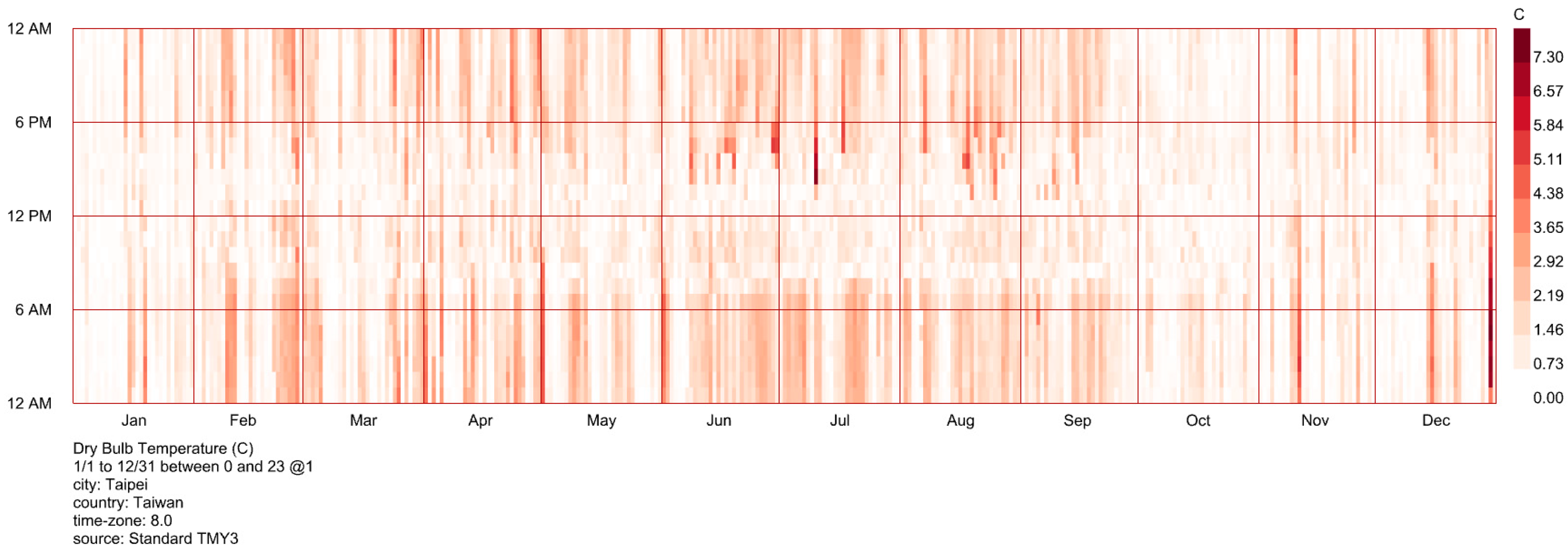
The results presented in Figure 3 illustrate the dry-bulb temperature distribution difference between the Taipei TMY3 and the UWG-modified TMY3. As observed in the figure, the differences between the weather files were more pronounced during the spring and summer months. The average air temperature difference between the standard Taipei TMY3 and the UWG-modified TMY3 was 0.63 °C. From Table 5, the values of kurtosis for the rural TMY indicate a smaller gap between the mode and the mean (4.27 °C) compared to the modified TMY (5.23 °C). With the additional consideration of anthropogenic heat flux and the urban setting within the UWG, the resulting average temperature exhibited a slight increase compared to rural areas (TMY3). This was due to the impact of urban heat.

3.2. ENVI-Met-Simulated Microclimate Results

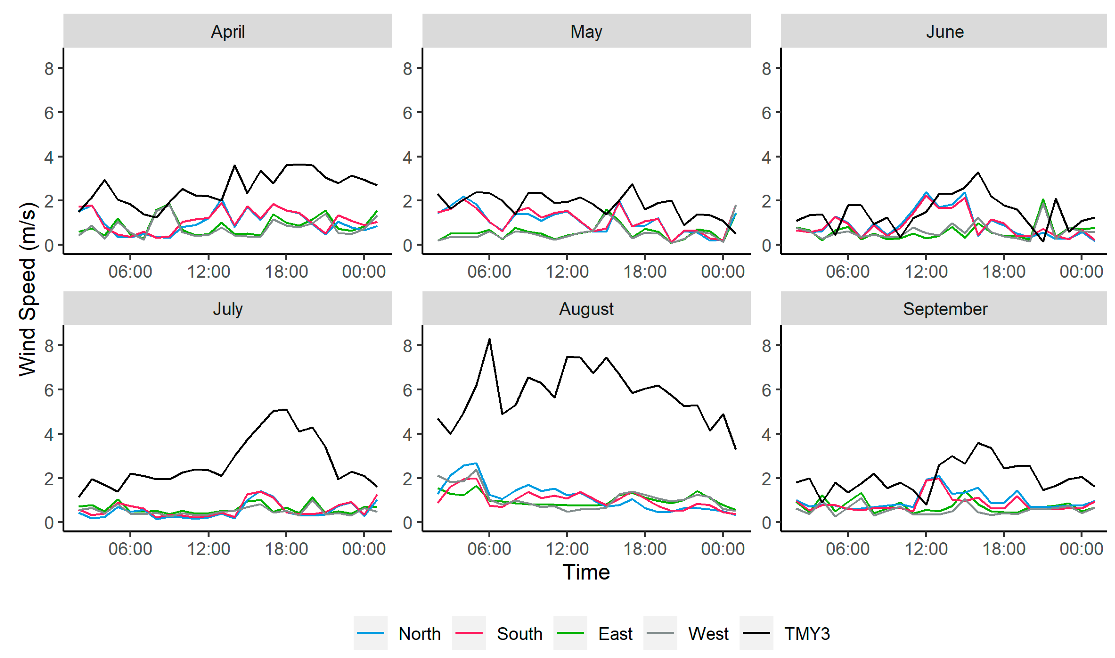
The months between April and September are presented based on their energy consumption intensity. A summary of the average wind speed results from ENVI-met is presented in Figure 4. These average values were obtained by averaging the simulation results from the coldest and the hottest days within each month. The figure distinctly indicates higher wind speeds in TMY3 compared to those in ENVI-met across all months. The wind speed values from ENVI-met ranged between 0.08 and 2.68 m/s. Values from the TMY3 ranged between 0.15 and 8.30 m/s, with an average wind speed of 2.66 m/s. In August, the wind speed was the highest for both the TMY3 and ENVI-met results. The average wind speed for the TMY3 was almost 3.5 times higher compared to the ENVI-met values. It is known that trees also have a strong influence on the wind speed distribution if as they act as porous media and induce pressure losses [17]. Such results from ENVI-met might be attributed to the presence of 15 m trees surrounding the target building; the canopies of trees obstructed the wind flow, resulting in reduced wind velocity.
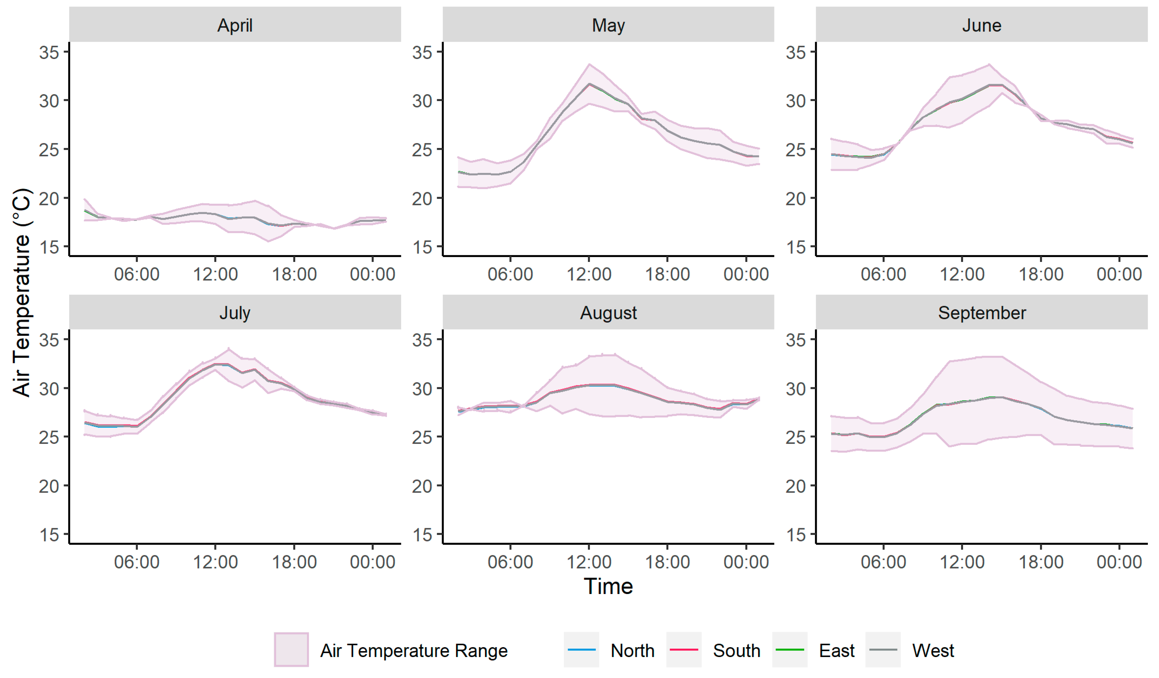
The ENVI-met air temperature results in Figure 5 show the hottest (top of ribbon), coldest (bottom of ribbon), and average (middle of ribbon) air temperature results from April to July. The reason for the overlap of the values was attributed to the identical features that all façade in the model shared. Comparing the wind speed values presented in Figure 4 and the air temperatures in Figure 5, it becomes more apparent that a decreasing wind speed generally coincided with an increasing air temperature. Similar findings have also been reported by Albatayneh et al. [55].

3.3. Results of BCVTB-Coupled Simulations

3.3.1. Surface Temperature

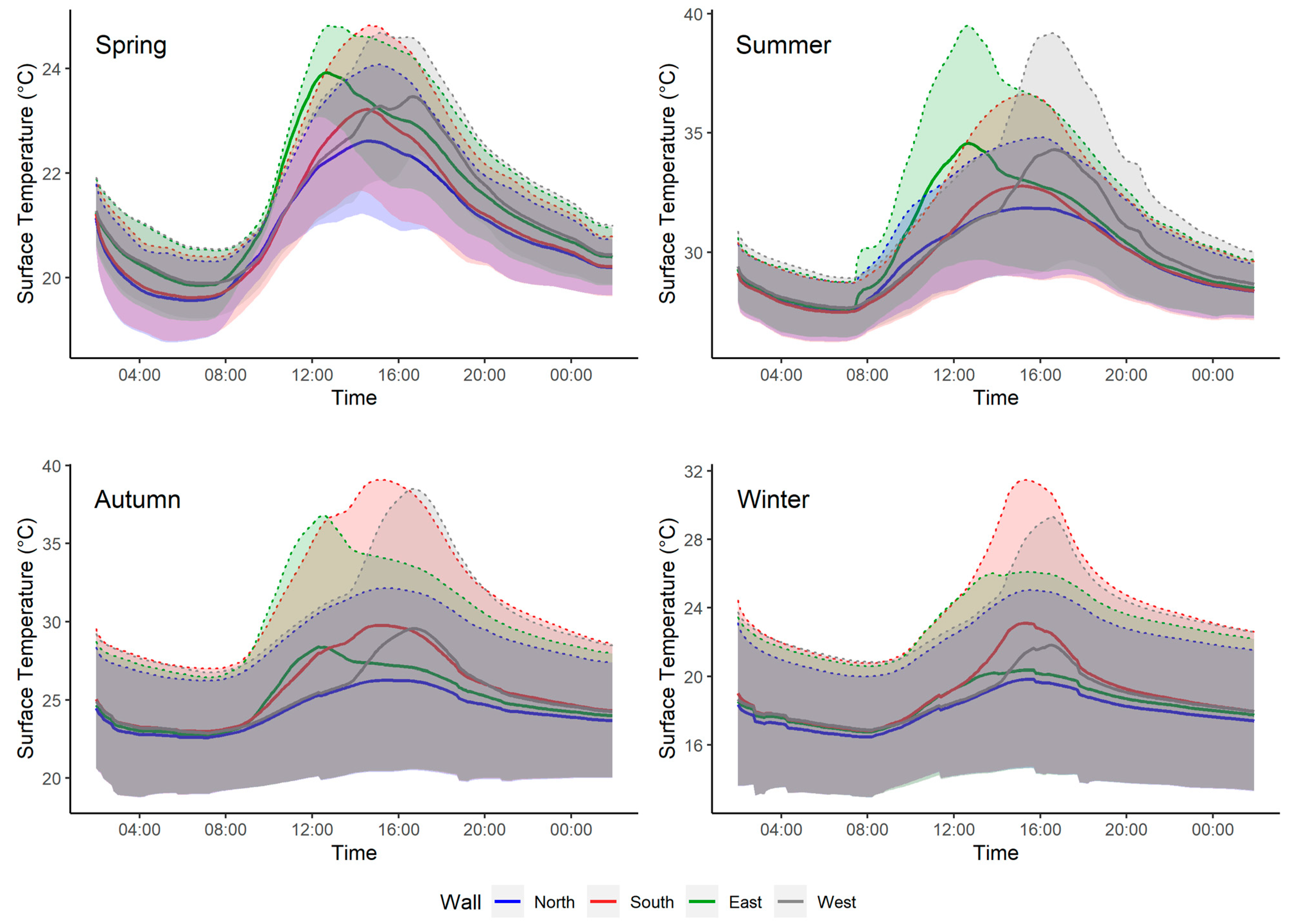
The surface temperature of the building walls resulting from BCVTB simulations is summarized in Figure 6. The upper dotted lines of the ribbon plots represent the average surface temperature on the hottest day of each month, while the lower bounds depict those on the coldest day. The solid-line curves are the average surface temperature values from the coldest and hottest days. The surface temperatures across all seasons ranged between 39.44 °C and 12.94 °C. Both the highest and the lowest surface temperatures were recorded on the east-facing wall. The season with the greatest deviation between the surface temperature results from cold and hot days was autumn, with south-facing walls having a difference of 20.31 °C. The mean surface temperature values for north, south, east, and west walls differed by less than 0.5 °C. It is also apparent that for the spring and summer seasons, eastern-facing walls were the hottest, with average surface temperatures of 20.74 °C and 30.29 °C. The autumn and winter months were characterized by larger surface temperature differences between the upper and the lower bounds of the ribbon plots, which coincided with a smoother normal distribution curve for hot days and an almost invariable surface temperature change for cold days. The hottest surfaces for the autumn and winter months were southern surfaces, followed by those on the west. The peak surface temperatures for southern walls were 39.08 °C and 31.36 °C for autumn and winter, respectively.

3.3.2. EnergyPlus-Only CHTC vs BCVTB-Coupled CHTC

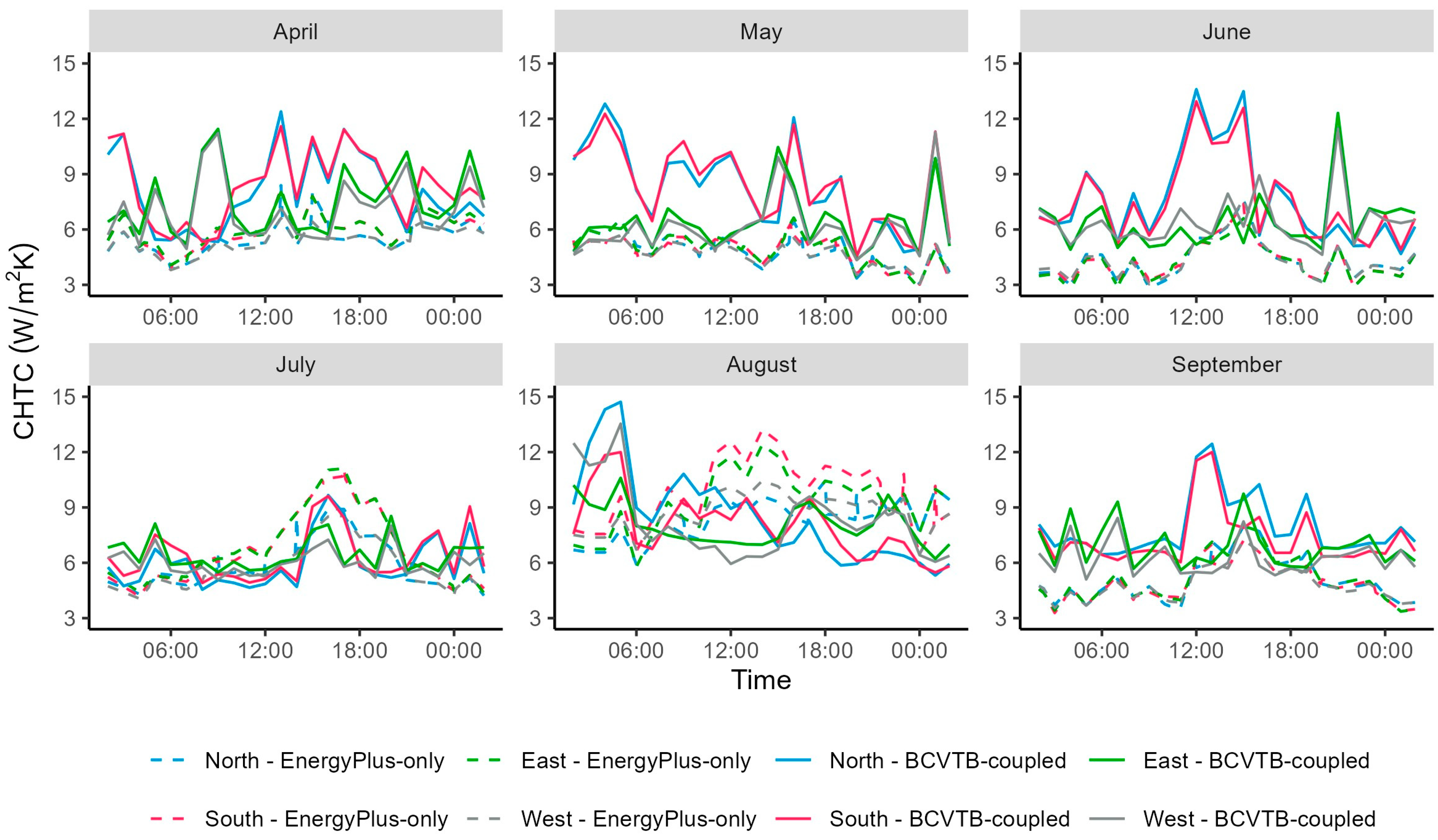
The results of the CHTC values generated by the BCVTB coupling were averaged for the relevant months and are presented in Figure 7. These values were produced from finding the mean between the coldest and hottest day of each month. The CHTC values from EnergyPlus were produced using the TARP method. The ENVI-met wind speed and CHTC were collinear due to the CHTC equation from ISO 6946 used in the coupling. The results show that the BCVTB-generated CHTC values were mostly higher than the EnergyPlus–TARP-generated CHTC values. The average CHTC from BCVTB was 7.02 W/m2·K, and it was 6.19 W/ m2·K with EnergyPlus. The highest CHTC values for both simulation methods were in August, though at different solar hours. The range of values for both were also similar, being around 10.4 W/m2K between the smallest and the largest values. The variation in CHTC values derived from TARP in EnergyPlus was due to most of the existing correlations being sensitive to windy environments [56]. The wind data from the TMY3 was recorded from an open space where velocities varied largely throughout the day. Despite the differences in values, there seemed to be some general similarity in the oscillation of the EnergyPlus-only CHTC and the BCVTB-coupling-generated CHTC values. Such urban topologies are known to reduce wind velocity [57].

3.3.3. CHTC vs. Surface Temperature

From the surface temperature results presented in Section 3.3.1, it is evident that the BCVTB simulation framework produced values that deviated from the EnergyPlus simulations due to the microclimate effect. As determined by many studies before, one of the ways buildings interact with their environment is via convective heat transfer [51,58,59]. To analyze the possible dynamics of the CHTC values and surface temperature, violin plots were produced that represent the surface temperature range of each façade and also its density (number of values per temperature term), as shown in Figure 8. Inside the violin plots are also boxplots that have lower and upper hinges that correspond to the first and third quartiles of the surface temperature values. The days presented in the figure were selected based on air temperature extremes, i.e., the coolest and the warmest months, February and July, respectively. For the coolest day in July, relatively large CHTC values populated the north, south, and west façades, with some values being as high as 14.34 W/m2·K. Since the violin plots also indicate the surface temperature that the CHTC values corresponded to, it can be observed that the larger the CHTC points, the smaller the surface temperature range. February 26th had the smallest CHTC values of all the months, especially for the western and eastern façades. These figures were also paired to some of the highest surface temperature values for winter months, which were as high as 37.10 °C for the southern wall. This can be attributed to the high air temperature values for February. The date 31 July, being the hottest summer day, had the largest surface temperature values along with the smallest CHTC, with a median of 5.7 W/m2·K. The presented observations show a common phenomenon, where larger surface temperature values correlated with smaller CHTC values. This seems to show that although higher values increase the heat transfer between a building and its immediate environment, a higher wind velocity also means that the heat accumulated in locales adjacent to the building can be removed more quickly [26,60].

3.3.4. BCVTB Surface Temperature Results Uncertainty Analysis

Various statistical measures can be used to perform error analysis of the BCVTB system’s surface temperature results against the standard EnergyPlus simulation surface temperature. These two error terms are the mean absolute error (MAE) and mean bias error (MBE) [61]. Assuming that h m , i is the i -th value of the surface temperature generated by EnergyPlus, h p , i is the i -th value of the surface temperature generated by the BCVTB model, and m is a total number of generated values from the EnergyPlus simulations, these can be obtained by the following equations:
MAE   = 1 m   i = 1 m h p , i   -   h m , i
MBE   = 1 m   i = 1 m h p , i   -   h m , i .
The mean absolute error (MAE) shows the average magnitude of the deviations of a modelled variable against the reference values. A low MAE indicates a high accuracy of a model. The MBE is used to determine the overall bias of the correlation. A positive MBE indicates the overestimation of a model [62]. The results from the error analysis of the surface temperature results from BCVTB and EnergyPlus are summarized in Table 6. The error analysis assumed that the EnergyPlus results represent the reference values and that the BCVTB results represent modelled variables. As such, negative or positive values for the MBE or MAE were not seen as an underestimation or an overestimation by the BCVTB but rather as a deviation resulting from accounting for the microclimate. In addition to using the average surface temperature values, the minimum and the maximum values were used to minimize the loss of resolution using average values. The average results showed the MAE values differing by approximately 0.26 °C for surfaces. Comparing these MAE values to those using the hottest days of the year, the deviations doubled. For the hottest days of year, there were differences of up to 0.65 °C. Using the coldest days of the year, such differences were slightly less, at around half a degree Celsius. Such small MAE values should normally indicate a high accuracy of the model. In this case, however, larger values indicated that the BCVTB results were substantially different to those of EnergyPlus. A potential cause for such small deviations between the surface temperature results from the two systems may be that the modified microclimate parameters did not differ too vastly from a normal case scenario. Recalling the results presented in Section 3.1, differences between the overall air temperatures were evident, but the maximum air temperature values were the same. The average air temperatures from both weather files differed by less than 1 °C.

4. Discussion

4.1. Urban Canyon Microclimate Conditions with and without Street Trees

To show the effect of street trees on the microclimate, all vegetation from the model was removed, and the BCVTB simulations were re-simulated and compared with the original case study. Figure 9a,b represent the diurnal surface temperature variation for May during daytime and nighttime, respectively. The difference between the surface temperatures of both BCVTB simulations was plotted for each month and is represented as ΔT (°C) in Figure 10. The results presented in Figure 9 and Figure 10 only show the surface temperatures of the hottest days of the months, which are typically energy-intensive. It can be observed that surface temperatures were higher for the BCVTB simulations where the vegetation was removed. This is a clear indication that trees play a pivotal role in mitigating high surface temperatures. The surface temperature differences ranged from 0.003 °C to 9.5 °C and were the largest for the hottest day in July on the western and eastern façades. The surface temperature differences minimized closer to the winter and spring months. The differences in surface temperatures for May were around 1.5 °C, while they were over 9 °C for some surfaces in July, indicating that the effectiveness of heat mitigation by trees differs depending on the time of the year. During summertime, properly placed trees tend to block unwanted solar radiation from striking buildings, which helps in reducing surface temperatures.
As it transitions from summer to colder seasons, the impact of trees on surface temperatures diminishes, coinciding with reduced incoming solar radiation and cooler ambient temperatures. Interestingly, during nighttime and early morning hours, the surface temperatures with trees were higher than those without trees, as evident in Figure 9b and Figure 10. Notably, the negative ΔT values below the horizontal dotted line in Figure 10 indicate that the BCVTB surface temperatures with trees exceeded those without trees. This nocturnal effect suggests that trees tend to obstruct the dissipation of heat from building surfaces to the cooler sky and surroundings during nighttime. This phenomenon aligns with observations made by Bouyer et al. [10] and Yang et al. [18] in their studies on the microclimate effects of urban vegetation on building cooling energy consumption. This suggests that street trees contribute to daytime cooling by obstructing incoming solar radiation through their canopy while also retaining nocturnal warmth [63]. This nocturnal warming effect is achieved as their canopy functions akin to a blanket, limiting irradiation and convection towards the cooler sky.

4.2. Impacts of Microclimate Behavior on Cooling Energy Consumption

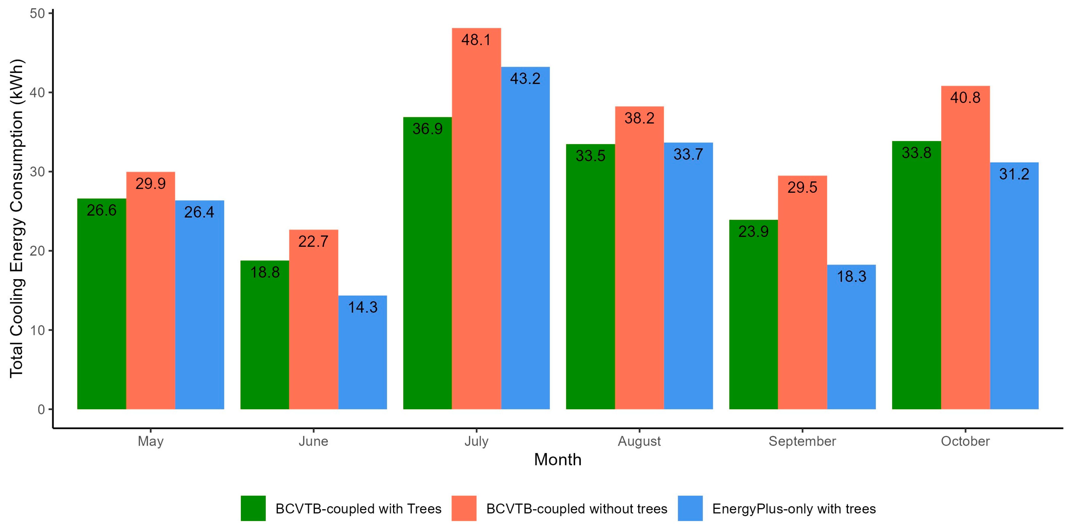
To assess the impact of the microclimate on the building cooling energy, we compared the results of the following simulation scenarios: (1) EnergyPlus-only simulations without coupling, (2) BCVTB-coupled simulations with trees, and (3) BCVTB-coupled simulations with all vegetation removed. Figure 11 presents the total cooling energy consumption for the three cases. Notably, the removal of vegetation had a significant effect on the building’s cooling load. For all the months considered, the BCVTB case without trees exhibited higher cooling energy requirements, underscoring the importance of shading effects and evapotranspiration in building energy consumption.
July was the month with the highest cooling energy consumption across all three simulation cases. The presence of trees on the hottest day in July led to a reduction in the cooling energy consumption by 11.2 kWh, equivalent to a 23.3% decrease. In July, the cooling energy demand reached 43.2 kWh, highlighting the critical role of trees in influencing the microclimate. However, considering trees solely as shading surfaces with a constant transmittance failed to capture their full cooling effect on the microclimate. The average cooling energy difference between the BCVTB simulations with trees and without trees was 17.3%. The BCVTB simulations without vegetation proved to be more energy-intensive than EnergyPlus-only simulations by an average of 25.2%. This shows that the presence of shading structures helps in reducing cooling energy consumption. These findings align with prior research, such as studies [11,18,26,59,64], demonstrating the substantial influence of microclimate conditions on cooling energy consumption in buildings, particularly in subtropical climates.

4.3. Contributions of the Proposed Coupling Method to the Trees’ Cooling Effect on the Building’s Cooling Energy

One of the primary advantages of this methodology over conventional studies concerning the effects of avenue trees on cooling energy is the modification of the weather file. The UWG offers a more detailed weather profile due to its inclusion of anthropogenic heat. Another advantage of using this system over other modification systems such as ENVI-met is that the computational power is almost negligible for the UWG. A more detailed morphology of the built environment is also possible with the UWG since its GUI is built within Rhinoceros. The average time of simulation is also a major advantage of the UWG, it being only 70 s for this study on an Acer i7-6700 CPU 16GB RAM laptop. ENVI-met simulations may take hours or even days depending on the size of the domain. The UWG is open-access and available in several different programming formats, which increases its versatility and applicability. Another advantage of the proposed method is the versatility of the coupling strategy within the BCVTB. The coupling can be modified to fit large-scale models, especially urban- or community-scale models. In this case, the effects of vegetation upon the cooling energy can be calculated at very high resolutions. At such scales, the effects of individual microclimate factors upon the energy consumption can be analyzed in a more detailed manner. Tsoka [25] also investigated energy demand using co-simulation on a comparable study area. The author demonstrated that cooling load variations of up to 28% were attributed to the presence of vegetation. However, the methodology adopted in that study involved a one-way approach, generating a new TMY from ENVI-met simulations and subsequently running standard EnergyPlus simulations. In contrast, the method employed in this study contains sophisticated computing algorithms that involve actuators that exchange vital microclimate factors at synchronized time steps, which create accurate thermophysical boundary conditions for energy simulations. Consequently, our simulations indicated an average cooling energy divergence of 17.3% between the BCVTB simulations conducted with and without trees from May to October. Furthermore, when comparing the BCVTB simulations incorporating trees against the EnergyPlus-only simulations, an average difference in cooling values of 23.4% was observed. Such differences in the resolution of the effect of greenery are imperative in understanding the complex nature of heat flux exchange between trees and the built environment. The warming and humidification effect of trees at nighttime in a hot-and-humid climate region can also be better understood using a coupling strategy. Considering that EnergyPlus assumes vegetation only as shading structures with no heat flux participation in the balance equations oversimplifies the effects of vegetation. Incorporating a microclimate-modifying aspect into the coupling strategy enhances the comprehension of this phenomenon and enables the assessment and seeking of strategies for effective approaches to reduce the adverse impacts of humidification on nighttime cooling loads while maximizing the cooling effect during the day.
There are a few shortcomings in this study that are worth mentioning. The UWG has certain simplifications in how vegetation is modelled. There is no change in the albedo of vegetation in the model during the change in seasons. There is simply the presence or absence of vegetation. Another limitation of this study is the computational intensity of generating microclimate data from ENVI-met. Though the simulation time may vary depending on the size of the domain, simulations may last anywhere from a few hours to days. There is also a location-specific data limitation. Due to the non-homogenous morphology of each urban area, CFD analysis is necessary for establishing boundary conditions. This puts a constraint on the scale and applicability of the proposed method. There is also the problem of simulation time incompatibility. The averaging of values attained from ENVI-met to deliver them to EnergyPlus limits the resolution and accuracy of performing microclimate simulations with ENVI-met. ENVI-met also does not consider the age of the trees or vegetation. It simply assumes that the vegetation is mature and that its biological functions are constant. The cooling benefits of trees are also dependent on annual stem growth variation across years and sites which are themselves influenced by underlying seasonal growth responses [65]. Etzold et al. [66] conducted a study that emphasized this phenomenon. The authors propose that forests or vegetation must be studied at a seasonal resolution in order gain insights into how plants grow and respond to climate change; accounting for the non-linear intra-annual growth dynamics would minimize uncertainties in the predictions of vegetation behavior, especially in the advent of climate change. The co-simulation model also has some challenges. One of the most important is that this type of coupling is a chaining method, which is method that does not exchange calculated variables from EnergyPlus back to ENVI-met for recalibration for the new iteration. This method is a one-way variable exchange. A more sophisticated model would involve a “strong coupling” strategy that addresses this shortcoming [20]. In such a method, the UCM and the BEM should bi-directionally exchange calculated variables simultaneously. The EnergyPlus Energy Management Actuators also have a limitation of 1024 values at any given simulation time, which makes it difficult to model very large buildings or complex buildings with many surfaces. Another limitation of the study is that it focuses only on vegetation as a UHI-mitigating strategy. The reality is that addressing urban heat involves many physical processes with complex interactions that range from building materials, heat from cooling plants, anthropogenic heat from all forms besides traffic, building topology, convection, etc. Zhao et al. [67] address this issue by proposing a ‘multimeasure-centric whole-system approach’ that contains solution sets comprising several mitigation measures rather than only one or a few. The authors not only considered the effectiveness of the solutions sets but also weighed the economic cost, which is often ignored. Another limitation of this study is that empirical analysis is lacking in this work. This and the previous limitations mentioned shall be addressed in future research.

5. Conclusions

This paper presents a methodology that bridges the gap between building energy simulation and urban climate modeling. To close this gap, the UCM software ENVI-met and the BES software EnergyPlus were coupled using the virtual test bed software BCVTB to account for microclimate factors that are imperative in the determining cooling energy consumption in buildings. An office building located in Taipei, Taiwan, was considered as the base-case scenario for this study. There are still challenges to implementing microclimate factors in building energy simulations to properly decipher a building’s interaction with its environment. A major issue is the lack of a general method to properly account for the microclimate parameters of a building and implementing these parameters in building energy simulation software to more accurately determine cooling energy needs. Some of the primary findings of this paper are as follows:
  • The UWG is an effective tool for modifying weather files, in that it accounts for the geometry of the local environment and anthropogenic heat flux, which is usually not considered in the modification of weather files for microclimate analysis. Such considerations increased the average air temperature of the weather file by 0.63 °C.
  • The coupling of microclimate factors from ENVI-met in EnergyPlus using the BCVTB provides an effective method for accounting for microclimate parameters in building energy simulation. Variables that determine the surface boundary conditions of a building, such as the wind speed and CHTC, are imperative in properly modeling the microclimate. Since most methods for determining the CHTC depend on correlations that are themselves dependent on local wind speed, these values had to be accounted for as accurately as possible using ENVI-met. The average wind speed for the TMY3 was almost 3.5 times higher compared to the ENVI-met values due to the open-space location where the data were collected. Comparing the CHTC values generated by TARP and the BCVTB-coupled system revealed an underestimation of these values on the part of EnergyPlus; the average values were 6.19 W/m2·K and 7.02 W/m2·K, respectively.
  • Comparing the EnergyPlus-only simulation and BCVTB simulation with trees with the EnergyPlus-only simulation and BCVTB simulation with removed vegetation revealed that the presence of trees decreased the cooling energy consumption. Notably, even when considering trees merely as transmittance surfaces within EnergyPlus, some level of shading was found to positively impact the reduction in building cooling energy requirements. The average building cooling energy difference between the BCVTB simulations with trees and without trees was 16.7%. Comparing the results from the BCVTB simulation with trees and the EnergyPlus-only simulation showed an underestimation of the cooling energy by EnergyPlus of about 9.3% on average for the summer months. However, the BCVTB simulation lacking vegetation exhibited even higher energy consumption, exceeding the EnergyPlus-only simulation by an average of 23.4%. These results underscore the role of shading structures in reducing cooling energy demand.
  • Surface temperatures were observed to rise in the BCVTB simulation after vegetation removal, with temperature increases of up to 9.5% during the hotter months. However, it is worth noting that the mitigating effect of trees on surface temperatures can be reversed during nighttime and early morning hours when heat is trapped beneath the tree canopy.

Author Contributions

Conceptualization, K.-T.H.; methodology, B.F. and K.-T.H.; software, B.F.; formal analysis, B.F.; resources, K.-T.H.; writing—original draft, B.F.; writing—review and editing, K.-T.H.; visualization, B.F.; supervision, K.-T.H.; project administration, K.-T.H.; funding acquisition, K.-T.H. All authors have read and agreed to the published version of the manuscript.

Funding

This research was funded by National Science and Technology Council of Taiwan, grant number MOST 109-2221-E-002-209-MY3.

Institutional Review Board Statement

Not applicable.

Informed Consent Statement

Not applicable.

Data Availability Statement

The raw data supporting the conclusions of this article will be made available by the authors upon request due to privacy concerns.

Conflicts of Interest

The authors declare no conflicts of interest.

Appendix A

Table A1. List of relevant variables and acronyms.
Nomenclature
VariablesAcronyms
q α sol Absorbed direct and diffuse solar radiation heat fluxANOVAAnalysis of variance
Q i n t e r n a l   l o a d s Building cooling/heating loadASHRAEAmerican Society of Heating, Refrigerating and Air-Conditioning Engineers
q c Convective heat transfer (W)AHFAnthropogenic heat flux
h c Convective heat transfer coefficient (W/m2·K)BCVTBBuilding Control Virtual Test Bed
q ko Conduction heat flux (q/A)BESBuilding energy simulation
E air Energy change of air in the zoneCHTCConvective heat transfer coefficient
ε Emissivity LADLeaf area density
q in Heat transfer due to infiltrationLAILeaf area index
q ihg Internal heat gainRLHTCRadiative linear heat transfer coefficient
q LWR Net longwave radiation heat exchangeRSMRural Station Model
h r Radiative linear heat transfer coefficient (W/m2·K)SHGCSolar heat gain coefficient
F sky Sky view factorTARPThermal Analysis Research Program
A Surface area (m2)TMYTypical meteorological year
σ Stefan–Boltzmann constant (W/m2·K4)UC-BEMUrban Canopy–Building Energy Model
T surf Temperature of building surface (°C)UBLUrban boundary layer
T air Temperature of outside air (°C)UWGUrban Weather Generator
v Wind speed (m/s)UHIUrban heat island
UCMUrban Climate Model
VDMVertical Diffusion Model
.idfEnergyPlus input data file
.epwEnergyPlus weather file

References

  1. Li, X.; Yao, R. Modelling heating and cooling energy demand for building stock using a hybrid approach. Energy Build. 2021, 235, 110740. [Google Scholar] [CrossRef]
  2. Grobman, Y.J.; Elimelech, Y. Microclimate on building envelopes: Testing geometry manipulations as an approach for increasing building envelopes’ thermal performance. Archit. Sci. Rev. 2016, 59, 269–278. [Google Scholar] [CrossRef]
  3. Corrado, V.; Ballarini, I. Refurbishment trends of the residential building stock: Analysis of a regional pilot case in italy. Energy Build. 2016, 132, 91–106. [Google Scholar] [CrossRef]
  4. Sola, A.; Corchero, C.; Salom, J.; Sanmarti, M. Simulation tools to build urban-scale energy models: A review. Energies 2018, 11, 3269. [Google Scholar] [CrossRef]
  5. Thermal Energy System Specialist (TESS). Trnsys, v18.0; Madison: Wisconsin, WI, USA, 2019. [Google Scholar]
  6. Ltd, D.B.S. Designbuilder, v7.0; Gloucs: Stroud, UK, 2021. [Google Scholar]
  7. Strachan, P. Esp-r, v13.3.17; Energy Systems Research Unit (ESRU), University of Strathcylde: Glasgow, UK, 2016. [Google Scholar]
  8. Noel, J. Codyba v6.5—Dynamical Behaviour for Buildings; JNLOG Scientific Computing: Lyon, France, 2021. [Google Scholar]
  9. National Renewable Energy Laboratory (NREL). Energyplus™, v9.2.0; US Department of Energy: Washington, DC, USA, 2020. [Google Scholar]
  10. Bouyer, J.; Inard, C.; Musy, M. Microclimatic coupling as a solution to improve building energy simulation in an urban context. Energy Build. 2011, 43, 1549–1559. [Google Scholar] [CrossRef]
  11. de la Flor, F.S.; Domínguez, S.A. Modelling microclimate in urban environments and assessing its influence on the performance of surrounding buildings. Energy Build. 2004, 36, 403–413. [Google Scholar] [CrossRef]
  12. Kawai, H.; Saito, R.; Sato, R. Numerical Study: How Does a High-Rise Building Affect the Surrounding Thermal Environment by Its Shading? CEPT University: Ahmedabad, India, 2014. [Google Scholar]
  13. Kesten, D.; Tereci, A.; Strzalka, A.M.; Eicker, U. A method to quantify the energy performance in urban quarters. HVACR Res. 2012, 18, 100–111. [Google Scholar] [CrossRef]
  14. Strømann-Andersen, J.; Sattrup, P.A. The urban canyon and building energy use: Urban density versus daylight and passive solar gains. Energy Build. 2011, 43, 2011–2020. [Google Scholar] [CrossRef]
  15. Frayssinet, L.; Merlier, L.; Kuznik, F.; Hubert, J.-L.; Milliez, M.; Roux, J.-J. Modeling the heating and cooling energy demand of urban buildings at city scale. Renew. Sustain. Energy Rev. 2018, 81, 2318–2327. [Google Scholar] [CrossRef]
  16. Yüksek, I.; Karadayi, T. Energy-efficient building design in the context of building life cycle. Energy Effic. Build. 2017, 10, 93–123. [Google Scholar]
  17. Morille, B.; Lauzet, N.; Musy, M. Solene-microclimate: A tool to evaluate envelopes efficiency on energy consumption at district scale. Energy Procedia 2015, 78, 1165–1170. [Google Scholar] [CrossRef]
  18. Yang, X.; Zhao, L.; Bruse, M.; Meng, Q. An integrated simulation method for building energy performance assessment in urban environments. Energy Build. 2012, 54, 243–251. [Google Scholar] [CrossRef]
  19. Laboratory, L.B.N. Building Control Virtual Test Bed (bcvtb), v1.6.0; DOE: Washington, WA, USA, 2016. [Google Scholar]
  20. Lauzet, N.; Rodler, A.; Musy, M.; Azam, M.-H.; Guernouti, S.; Mauree, D.; Colinart, T. How building energy models take the local climate into account in an urban context—A review. Renew. Sustain. Energy Rev. 2019, 116, 109390. [Google Scholar] [CrossRef]
  21. Ramesh, S. Urban Energy Information Modeling: A Framework to Quantify the Thermodynamic Interactions between the Natural and the Built Environment that Affect Building Energy Consumption. Ph.D. Thesis, Carnegie Mellon University, Pittsburgh, PA, USA, 2018. [Google Scholar]
  22. Wetter, M. Co-simulation of building energy and control systems with the building controls virtual test bed. J. Build. Perform. Simul. 2011, 4, 185–203. [Google Scholar] [CrossRef]
  23. Kharbouch, A.; Berrabah, S.; Bakhouya, M.; Gaber, J.; El Ouadghiri, D.; Idrissi Kaitouni, S. Experimental and co-simulation performance evaluation of an earth-to-air heat exchanger system integrated into a smart building. Energies 2022, 15, 5407. [Google Scholar] [CrossRef]
  24. Miguel, M.; Hien, W.N.; Marcel, I.; Jun Chung, H.D.; Yueer, H.; Zhonqi, Y.; Ji-Yu, D.; Raghavan, S.V.; Son, N.N. A physically-based model of interactions between a building and its outdoor conditions at the urban microscale. Energy Build. 2021, 237, 110788. [Google Scholar] [CrossRef]
  25. Tsoka, S. Evaluating the impact of urban microclimate on buildings’ heating and cooling energy demand using a co-simulation approach. Atmosphere 2023, 14, 652. [Google Scholar] [CrossRef]
  26. Huang, K.-T.; Li, Y.-J. Impact of street canyon typology on building’s peak cooling energy demand: A parametric analysis using orthogonal experiment. Energy Build. 2017, 154, 448–464. [Google Scholar] [CrossRef]
  27. Chen, Y.-C.; Lo, T.-W.; Shih, W.-Y.; Lin, T.-P. Interpreting air temperature generated from urban climatic map by urban morphology in taipei. Theor. Appl. Climatol. 2019, 137, 2657–2662. [Google Scholar] [CrossRef]
  28. Hwang, R.-L.; Lin, C.-Y.; Huang, K.-T. Spatial and temporal analysis of urban heat island and global warming on residential thermal comfort and cooling energy in taiwan. Energy Build. 2017, 152, 804–812. [Google Scholar] [CrossRef]
  29. Bueno, B.; Norford, L.; Hidalgo, J.; Pigeon, G. The urban weather generator. J. Build. Perform. Simul. 2013, 6, 269–281. [Google Scholar] [CrossRef]
  30. Bueno, B.; Nakano, A.; Norford, L.; Reinhart, C. Urban Weather Generator—A Novel Workflow for Integrating Urban Heat Island Effect within Urban Design Process; International Building Performance Simulation Association: Fairfax, VA, USA, 2015. [Google Scholar]
  31. Yang, J.H. The Curious Case of Urban Heat Island: A Systems Analysis; MITLibraries: Cambridge, MA, USA, 2016. [Google Scholar]
  32. Bueno, B.; Nakano, A.; Norford, L. Urban weather generator: A method to predic neighborhood-specific urban temperatures for use in building energy simulations. In Proceedings of the ICUC9—9th International Conference on Urban Climate jointly with 12th Symposium on the Urban Environment, Toulouse, France, 20–24 July 2015. [Google Scholar]
  33. Lin, C.-Y.; Chen, F.; Huang, J.C.; Chen, W.C.; Liou, Y.A.; Chen, W.N.; Liu, S.-C. Urban heat island effect and its impact on boundary layer development and land–sea circulation over northern taiwan. Atmos. Environ. 2008, 42, 5635–5649. [Google Scholar] [CrossRef]
  34. Koralegedara, S.B.; Lin, C.-Y.; Sheng, Y.-F.; Kuo, C.-H. Estimation of anthropogenic heat emissions in urban taiwan and their spatial patterns. Environ. Pollut. 2016, 215, 84–95. [Google Scholar] [CrossRef] [PubMed]
  35. Ladybug Tools LLC. Ladybug Tools (LBT), v1.2.0; Ladybug Tools LLC: Fairfax, VA, USA, 2021. [Google Scholar]
  36. Quah, A.K.L.; Roth, M. Diurnal and weekly variation of anthropogenic heat emissions in a tropical city, singapore. Atmos. Environ. 2012, 46, 92–103. [Google Scholar] [CrossRef]
  37. Bueno, B.; Roth, M.; Norford, L.; Li, R. Computationally efficient prediction of canopy level urban air temperature at the neighbourhood scale. Urban Clim. 2014, 9, 35–53. [Google Scholar] [CrossRef]
  38. TomTom. Taiwan: Taipei Traffic. 2017. Available online: https://www.tomtom.com/traffic-index/taipei-traffic/ (accessed on 11 June 2017).
  39. Alchapar, N.; Pezzuto, C.; Correa, E.; Salvati, A. Thermal performance of the urban weather generator model as a tool for planning sustainable urban development. Geogr. Pannonica 2019, 23, 374–384. [Google Scholar]
  40. Palme, M.; Inostroza, L.; Villacreses, G.; Lobato, A.; Carrasco, C. Urban weather data and building models for the inclusion of the urban heat island effect in building performance simulation. Data Brief 2017, 14, 671–675. [Google Scholar] [CrossRef]
  41. Martien, P.; Akbari, H.; Rosenfeld, A. Light colored surfaces to reduce summertime urban temperatures: Benefits, costs, and implementation issues. In Proceedings of the 9th Miami Internation Congress on Energy and Environment, Miami Beach, FL, USA, 11–13 December 1989. [Google Scholar]
  42. Bretz, S.; Akbari, H.; Rosenfeld, A.; Taha, H. Implementation of Solar-Reflective Surfaces: Materials and Utility Programs; Lawrence Berkeley National Laboratory: Berkeley, CA, USA, 1992; pp. 1–73, LBL-32467: OSTI ID:10172670. [Google Scholar]
  43. Baker, M.C. Roofs: Design, Application and Maintenance; Polyscience Publications: Québec, QC, Canada, 1980. [Google Scholar]
  44. Sailor, D.J. A review of methods for estimating anthropogenic heat and moisture emissions in the urban environment. Int. J. Climatol. 2011, 31, 189–199. [Google Scholar] [CrossRef]
  45. Corrado, V.; Fabrizio, E. Chapter 5—Steady-state and dynamic codes, critical review, advantages and disadvantages, accuracy, and reliability. In Handbook of Energy Efficiency in Buildings; Asdrubali, F., Desideri, U., Eds.; Butterworth-Heinemann: Oxford, UK, 2019; pp. 263–294. [Google Scholar]
  46. Toparlar, Y.; Blocken, B.; Maiheu, B.; van Heijst, G.J.F. A review on the cfd analysis of urban microclimate. Renew. Sustain. Energy Rev. 2017, 80, 1613–1640. [Google Scholar] [CrossRef]
  47. Gros, A.; Bozonnet, E.; Inard, C. Cool materials impact at district scale—Coupling building energy and microclimate models. Sustain. Cities Soc. 2014, 13, 254–266. [Google Scholar] [CrossRef]
  48. Castaldo, V.L.; Pisello, A.L.; Piselli, C.; Fabiani, C.; Cotana, F.; Santamouris, M. How outdoor microclimate mitigation affects building thermal-energy performance: A new design-stage method for energy saving in residential near-zero energy settlements in italy. Renew. Energy 2018, 127, 920–935. [Google Scholar] [CrossRef]
  49. Tsoka, S.; Tsikaloudaki, A.; Theodosiou, T. Analyzing the envi-met microclimate model’s performance and assessing cool materials and urban vegetation applications–a review. Sustain. Cities Soc. 2018, 43, 55–76. [Google Scholar] [CrossRef]
  50. Hyl, C.; Lee, E.; Liu, J.; Neuendorffer, S.; Cheong, E.; John, H.; Tsay, J.; Vogel, B.; Williams, W.; Xiong, Y.; et al. Ptolemy II: Heterogeneous Concurrent Modeling and Design in Java. In Document v2.0.1; Memorandum UCB/ERL M02/23; University of California: Berkeley, CA, USA, 2002. [Google Scholar]
  51. Shen, P.; Dai, M.; Xu, P.; Dong, W. Building heating and cooling load under different neighbourhood forms: Assessing the effect of external convective heat transfer. Energy 2019, 173, 75–91. [Google Scholar] [CrossRef]
  52. Zhong, W.; Zhang, T.; Tamura, T. Cfd simulation of convective heat transfer on vernacular sustainable architecture: Validation and application of methodology. Sustainability 2019, 11, 4231. [Google Scholar] [CrossRef]
  53. ISO 6946: 2007; Building Components and Building Elements—Thermal Resistance and Thermal Transmittance—Calculation Method. International Organization for Standardization: Geneva, Switzerland, 2007.
  54. Wetter, M.; Nouidui, T.S. Building Controls Virtual Test Bed User Manual, v1.6.0; Lawrence Berkeley National Laboratory (LBNL): Berkely, CA, USA; Department of Energy: Washington, DC, USA, 2016; p. 90. [Google Scholar]
  55. Albatayneh, A.; Alterman, D.; Page, A.; Moghtaderi, B. Alternative method to the replication of wind effects into the buildings thermal simulation. Buildings 2020, 10, 237. [Google Scholar] [CrossRef]
  56. Kahsay, M.; Bitsuamlak, G.; Tariku, F. Effect of localized exterior convective heat transfer on high-rise building energy consumption. Build. Simul. 2019, 13, 127–139. [Google Scholar] [CrossRef]
  57. Szkordilisz, F.; Zöld, A. Effect of vegetation on wind-comfort. Appl. Mech. Mater. 2016, 824, 811–818. [Google Scholar] [CrossRef]
  58. Montazeri, H.; Blocken, B.; Derome, D.; Carmeliet, J.; Hensen, J.L.M. Cfd analysis of forced convective heat transfer coefficients at windward building facades: Influence of building geometry. J. Wind. Eng. Ind. Aerodyn. 2015, 146, 102–116. [Google Scholar] [CrossRef]
  59. Vallati, A.; Vollaro, A.D.L.; Golasi, I.; Barchiesi, E.; Caranese, C. On the impact of urban micro climate on the energy consumption of buildings. Energy Procedia 2015, 82, 506–511. [Google Scholar] [CrossRef]
  60. Huang, C.-H.; Tsai, H.-H.; Chen, H.-c. Influence of weather factors on thermal comfort in subtropical urban environments. Sustainability 2020, 12, 2001. [Google Scholar] [CrossRef]
  61. Yin, C.-Y. Prediction of higher heating values of biomass from proximate and ultimate analyses. Fuel 2011, 90, 1128–1132. [Google Scholar] [CrossRef]
  62. Michalak, P. Experimental and theoretical study on the internal convective and radiative heat transfer coefficients for a vertical wall in a residential building. Energies 2021, 14, 5953. [Google Scholar] [CrossRef]
  63. Zhao, Y.; Li, H.; Bardhan, R.; Kubilay, A.; Li, Q.; Carmeliet, J. The time-evolving impact of tree size on nighttime street canyon microclimate: Wind tunnel modeling of aerodynamic effects and heat removal. Urban Clim. 2023, 49, 101528. [Google Scholar] [CrossRef]
  64. Allegrini, J.; Dorer, V.; Carmeliet, J. Influence of the urban microclimate in street canyons on the energy demand for space cooling and heating of buildings. Energy Build. 2012, 55, 823–832. [Google Scholar] [CrossRef]
  65. Sellier, D.; Ségura, R. Radial growth anisotropy and temporality in fast-growing temperate conifers. Ann. For. Sci. 2020, 77, 85. [Google Scholar] [CrossRef]
  66. Etzold, S.; Sterck, F.; Bose, A.K.; Braun, S.; Buchmann, N.; Eugster, W.; Gessler, A.; Kahmen, A.; Peters, R.L.; Vitasse, Y.; et al. Number of growth days and not length of the growth period determines radial stem growth of temperate trees. Ecol. Lett. 2022, 25, 427–439. [Google Scholar] [CrossRef]
  67. Zhao, Y.; Sen, S.; Susca, T.; Iaria, J.; Kubilay, A.; Gunawardena, K.; Zhou, X.; Takane, Y.; Park, Y.; Wang, X.; et al. Beating urban heat: Multimeasure-centric solution sets and a complementary framework for decision-making. Renew. Sustain. Energy Rev. 2023, 186, 113668. [Google Scholar] [CrossRef]
Figure 1. Overview of research methodology.
Atmosphere 15 01150 g001
Figure 2. Case study building model: (a) the 3D building is enclosed by structures on all sides that represent other buildings or surfaces in EnergyPlus; (b) the building model in ENVI-met: the location of the target building that is surrounded by adjacent buildings of a similar structure and trees that are equidistant.
Atmosphere 15 01150 g002
Figure 3. The difference between the dry-bulb temperature profile of the TMY3 (avg. T of 23.33 °C) and the dry-bulb temperature profile of the UWG-produced weather file (avg. T of 23.96 °C).
Atmosphere 15 01150 g003
Figure 4. ENVI-met average wind speed results for north, south, east, and west façades of building model and the wind speed results of the standard TMY3 for Taipei.
Atmosphere 15 01150 g004
Figure 5. Summary of ENVI-met ambient air temperature results: the line in the plot is the average temperature that was calculated by averaging the hottest and coldest day values; the hottest and coldest days are also shown as the upper and lower lines, respectively.
Atmosphere 15 01150 g005
Figure 6. BCVTB surface temperature results for spring (top left), summer (top right), autumn (bottom left), and winter (bottom right) months. The ribbon plots show the upper and lower bounds of surface temperature results, which were carried out for the hottest and coldest days of each month.
Atmosphere 15 01150 g006
Figure 7. Average CHTC results from coldest and hottest days of April to September months from EnergyPlus simulations and BCVTB-coupled simulations.
Atmosphere 15 01150 g007
Figure 8. Violin plots of days that contained the hottest surface temperatures of the year. The violin plots are also density plots that represents the frequency of surface temperature values on the y-axis. The red dots in the boxplot are the median surface temperature values. Colored dots represent the CHTC values and the corresponding surface temperature for that timestep.
Atmosphere 15 01150 g008
Figure 9. BCVTB surface temperature comparison between surface temperatures from simulations with trees and without trees for May: (a) daytime surface temperature variation for May; (b) nighttime surface temperature variation.
Atmosphere 15 01150 g009
Figure 10. Surface temperature difference (ΔT) between BCVTB simulations with trees and without trees for months that require cooling energy.
Atmosphere 15 01150 g010
Figure 11. Total cooling energy consumption comparison between BCVTB-coupled simulation with trees, BCVTB-coupled simulation without trees, and EnergyPlus-only simulation cooling energy.
Atmosphere 15 01150 g011
Table 2. Settings of EnergyPlus simulations.
SettingsValues
LocationTaipei City, latitude: 25.02; longitude: 121.54)
Area of building2000 m2
Window glazingU value (W/m2k) = 6.07
SHGC = 0.8
Window-to-wall ratio (WWR) = 0.4
Weather filesUWG generated/modified TMY3
Simulation period1 year (365 days)
Internal loadOccupancy (people/m2) = 0.15
Lighting (W/m2) = 15
Electric equipment (W/m2) = 10
HVAC systemVariable air volume (VAV)
Chiller COP = 5.0
Cooling setpoint: 24 °C
Heating setpoint: none
Surface convection algorithmTARP [Table A1]
Ground reflectance and temperatureENVI-met output data
TreesTransmittance: 0.07
Table 3. Settings of ENVI-met simulations from the configuration file.
SettingsValues
Domain120 m × 120 m × 18 m
Mesh sizedx = 2 m, dy = 2 m, dz = 2 m
EnvironmentWith greenery
TreesGeneral structure: cylindric, large trunk, dense, medium (15 m),
Albedo: 0.12,
LAI: 2.3 m2m2,
LAD: 2 m2m3
Foliage transmittance: 0.10,
Leaf type: conifer
Leaf weight: 100 g/m2
Depth of roots: 9 m
Diameter of roots: 7 m
CO2 fixation type: C3-Plant
Simulation periodColdest and hottest day of every month, January to December based on TMY3
Reference time zoneGMT + 8:00
Weather dataSimple forcing with data from Taipei TMY3
GroundAsphalt road—albedo: 0.2,
Concrete gray pavement—albedo: 0.5,
Loamy soil—albedo: 0.0
Table 4. Variables that are a part of the coupling solution and their source [21].
Variables Calculated in the Coupling PlatformInput Source
EnergyPlusENVI-Met
Absorbed direct and diffuse solar radiation (1)
Incident solar radiation
Shadowing effects
Convective flux change with outside air–
surface boundary conditions (2)
Surface temperature
Air temperature near surface
Wind speed
Longwave radiation flux
Outside surface temperature
Outside air temperature
Heat and Moisture via infiltration (3)
Infiltration schedule
Indoor zone air temperature
Outdoor dry-bulb temperature
Wind speed around building surface
Table 5. Descriptive statistics of air temperature values from rural Taipei TMY3 and the UWG-modified urban TMY3.
VariableTaipei TMY3 (Rural)UWG-Modified TMY3 (Urban)
Mean23.3323.96
Median23.824.4
Mode27.629.2
Standard Deviation5.655.74
Kurtosis−0.66−0.75
Range8.7~37.19.5~37.1
Table 6. Error terms and values for surface temperature of north, south, east, and west façades for the summer season.
MetricAverage ValuesMaximum ValuesMinimum Values
NorthSouthEastWestNorthSouthEastWestNorthSouthEastWest
MAE (°C)0.270.260.300.220.640.530.650.570.500.490.550.55
MBE (°C)−0.17−0.09−0.07−0.09−0.62−0.45−0.50−0.530.290.270.350.36
Disclaimer/Publisher’s Note: The statements, opinions and data contained in all publications are solely those of the individual author(s) and contributor(s) and not of MDPI and/or the editor(s). MDPI and/or the editor(s) disclaim responsibility for any injury to people or property resulting from any ideas, methods, instructions or products referred to in the content.