Article

High-Resolution Daily PM2.5 Exposure Concentrations in South Korea Using CMAQ Data Assimilation with Surface Measurements and MAIAC AOD (2015–2021)

Department of Environmental Engineering, Anyang University, Anyang-si 14028, Gyeonggi-do, Republic of Korea
*
Author to whom correspondence should be addressed.
Atmosphere 2024, 15(10), 1152; https://doi.org/10.3390/atmos15101152
Submission received: 14 August 2024 / Revised: 14 September 2024 / Accepted: 20 September 2024 / Published: 26 September 2024
(This article belongs to the Special Issue Novel Insights into Air Pollution over East Asia)

Abstract

:
Particulate matter (PM) in the atmosphere poses significant risks to both human health and the environment. Specifically, PM2.5, particulate matter with a diameter less than 2.5 micrometers, has been linked to increased rates of cardiovascular and respiratory diseases. In South Korea, concerns about PM2.5 exposure have grown due to its potential for causing premature death. This study aims to estimate high-resolution exposure concentrations of PM2.5 across South Korea from 2015 to 2021. We integrated data from the Community Multiscale Air Quality (CMAQ) model with surface air quality measurements, the Weather Research Forecast (WRF) model, the Normalized Difference Vegetation Index (NDVI), and the Multi-Angle Implementation of Atmospheric Correction (MAIAC) Aerosol Optical Depth (AOD) satellite data. These data, combined with multiple regression analyses, allowed for the correction of PM2.5 estimates, particularly in suburban areas where ground measurements are sparse. The simulated PM2.5 concentration showed strong correlations with observed values R (ranging from 0.88 to 0.94). Spatial distributions of annual PM2.5 showed a significant decrease in PM2.5 concentrations from 2015 to 2021, with some fluctuation due to the COVID-19 pandemic, such as in 2020. The study produced highly accurate daily average high-resolution PM2.5 exposure concentrations.

1. Introduction

Particulate matter (PM) in the atmosphere is known to affect not only the aerial ecosystem but also the natural ecosystem and climate change. It is particularly harmful to the human respiratory and cardiovascular systems. Exposure to PM2.5 (particulate matter with an aerodynamic diameter less than 2.5 micrometers) has been reported in numerous studies to increase the risk of cardiovascular and respiratory diseases as well as premature death [1]. The World Health Organization (WHO) reported that, in 2016, air pollution caused approximately 7 million deaths worldwide [2].
South Korea, having transitioned from a developing country through rapid industrialization, has recently introduced various air quality improvement policies in an effort to reduce PM concentrations. However, public anxiety over exposure to high levels of PM has been increasing, making this not just an environmental issue but also a social concern. Consequently, numerous studies have been conducted domestically on the health impacts of air pollution. For example, Hwang et al. (2018) analyzed the association between air quality and subjective stress using community health data [3], while Kim et al. (2018) reported that long-term exposure to PM2.5 could result in 17,233 premature deaths annually in South Korea [4]. Lim et al. (2016) found that short-term exposure to PM2.5 increases the risk of premature death from respiratory and cardiovascular diseases by a factor of 1.028 per 10 μ g / m 3 [5]. Furthermore, Kim et al. (2019) reported that air pollution reduction policies in Seoul have contributed to a decrease in hospital visits for asthma patients [6].
An assessment of the health impacts of air pollution in South Korea have primarily relied on national air quality monitoring network data, with exposure concentrations calculated around specific measurement sites. However, this approach has a limitation in terms of representativeness for regions without measurement data. Particularly, until 2014, the air quality monitoring network focused primarily on PM10, resulting in a lack of data on PM2.5, which is crucial for risk assessments. Therefore, a more accurate evaluation of the health risks posed by air pollution requires the estimation of more detailed spatiotemporal exposure data.
Methods for estimating exposure data include using ground-based air quality monitoring data with Land Use Regression (LUR) models, satellite data, chemical transport modeling, and fusion models (such as satellites with artificial intelligence or chemical transport models with artificial intelligence) to estimate exposure concentrations. The LUR model predicts pollution concentrations by correlating geographic variables that influence air pollution with air quality measurements [7,8]. LUR is relatively straightforward and effective in urban areas with abundant measurement data, but it tends to have higher errors in suburban areas with fewer measurements. Champendal et al. (2014) developed an LUR model that included land use information such as airports, population distribution, heating systems, and roads, and they used ground-based measurements to produce exposure concentrations through multiple linear regression [9]. However, in areas with low spatial resolution or missing data (without measurements), the model’s accuracy was limited. To overcome these limitations, the development of LUR models using satellite data has been actively pursued [10,11]. Stafoggia et al. (2019) estimated daily PM10 and PM2.5 concentrations in Italy for the period 2013–2015 using MODIS AOD, NDVI, weather data, land cover data, and ground measurements as input variables, applying Random Forests (RFs) to generate PM exposure concentrations [11]. To improve accuracy, efforts have been made to add new variables to the LUR model or to enhance the spatial and temporal variability of existing variables. For example, Ndiaye et al. (2024) used an LUR model to predict hourly concentrations of NO2 and PM2.5 in the Netherlands, producing hourly concentrations for these two pollutants from 2016 to 2019 [12]. Two methods, Supervised Linear Regression (SLR) and Random Forest, were employed, utilizing various predictor variables such as road density, population density, land use, and satellite observation data.
Satellite data provide the advantage of consistent spatial resolution across large areas, making them widely used in estimating air pollution exposure concentrations [13,14,15]. Recently, various correction techniques and algorithms have been introduced to enhance the utility of satellite data. However, satellite observations are limited to cloud-free daylight hours, resulting in lower temporal resolution. In fact, analysis of MODIS AOD data showed that, annually, less than 30% of the days were suitable for satellite data acquisition. Wang et al. (2022) pointed out that, while satellite-based AOD data are widely used to estimate PM2.5 concentrations, they often suffer from gaps due to clouds, snow, or air pollution, leading to limited spatial coverage [16]. To overcome these limitations, they proposed a new method that integrates satellite AOD data with smartphone-based estimates to more accurately predict PM2.5 concentrations. For the Korean region, Park et al. (2020) used a Random Forest (RF) approach to estimate spatially continuous Aerosol Optical Depth (AOD) and particulate matter (PM10, PM2.5) concentrations over East Asia [17]. Satellite data from the 2016 Geostationary Ocean Color Imager (GOCI) were combined with ancillary data for model development. The method performed the best (R2 0.74 for AOD and 0.88–0.90 for PM), effectively capturing the spatial and seasonal distribution of fine particles. The proposed method can reliably estimate AOD and PM under all sky conditions. Lee et al. (2021) presented a deep neural network (DNN) approach to monitor PM2.5 concentrations over the Korean Peninsula using GOCI satellite images and UM reanalysis data [18]. The DNN model was optimized through hyperparameter tuning, regularization, and early stopping to avoid overfitting. It outperformed conventional methods like Random Forest and multiple linear regression in both hold-out validation and cross-validation, with lower RMSE and MBE values, although high PM2.5 concentrations were slightly underestimated. The DNN’s accuracy shows the potential for reliable PM2.5 monitoring. Lee et al. (2022) utilized a machine learning (ML) algorithm, specifically Random Forest, to estimate ground-level particulate matter (PM) from GOCI satellite Aerosol Optical Depth (AOD) data [19]. The estimated PM was incorporated into a numerical air quality forecast model using data assimilation (DA), which significantly improved PM10 forecasts for up to 24 h and PM2.5 forecasts for up to 6 h. The combination of DA and ML proved highly effective in enhancing the accuracy of ground-level air quality predictions. Tang et al. (2024) uses a Random Forest machine learning model to predict daily PM2.5, O3, and NO2 concentrations over South Korea, integrating meteorology, satellite data, and chemical transport models. It achieved high predictive accuracy, validated using KORUS-AQ 2016 data and incorporating GEMS observations from 2021. The study also evaluated the impact of different reanalysis datasets and satellite AOD sources on prediction performance [20].
This study aimed to estimate the exposure concentrations of PM2.5, which are critical environmental factors for risk assessment. Various data were utilized to estimate exposure concentrations. To ensure high-quality spatial resolution, data assimilation modeling was performed using CMAQ modeling and air quality data from automatic monitoring networks in China and South Korea. However, data assimilation relies solely on ground-based air quality observations, which inherently limits representativeness in suburban areas where measurement data are lacking. To address this limitation and correct the results of data assimilation modeling, AOD data were used, and multiple regression analysis was applied, ultimately producing reanalyzed air quality data.
In summary, this study aims to generate daily average, high-resolution (1 km) PM2.5 exposure concentration data for the Korean Peninsula from 2015 to 2021 using multiple linear regression (MLR) by integrating CMAQ data assimilation, meteorological model data, AOD, and NDVI satellite datasets.

2. Measurement Data from Surface and Satellite

2.1. Air Quality Measurement Data

Air quality observation data are used as input data for chemical transport model data assimilation and multiple regression analysis. In this study, the locations of the automatic monitoring networks for air quality measurements in China (www.pm25.in, accessed on 11 August 2024) and South Korea (www.airkorea.or.kr, accessed on 11 August 2024) that were utilized are shown in Figure 1. The real-time air quality measurement data that can be collected in Northeast Asia includes 1492 sites in China and 444 sites in South Korea. The items measured in real time at these monitoring sites include PM10, PM2.5, NO2, SO2, CO, and O3. These data were used to perform data assimilation for chemical transport modeling. This study presents high-resolution PM2.5 concentrations in South Korea but, in order to include the more accurate impact of trans-boundary pollution from upwind areas, surface measurements from China were assimilated into the East Asia domain [21].

2.2. AOD and NDVI Satellite Observation Data

We utilized 1 km resolution AOD data (MCD19A2) obtained from the MODIS sensor onboard NASA’s Terra and Aqua satellites, processed using the MAIAC (Multi-Angle Implementation of Atmospheric Correction) algorithm [22,23]. For Level 2 MCD19A2 data, we used AOD values classified as best quality, which corresponds to cases where the CloudMask Adjacency Mask is clear, excluding adjacent data affected by clouds, snow, or ice. The overpass times of these satellites over the Korean Peninsula are 10:30 a.m. for Terra and 1:30 p.m. for Aqua, so the daily average AOD was calculated by averaging the AOD observations from both satellites. The NDVI data used were monthly data from MODIS Level 3, and to ensure sufficient data coverage across the entire Korean Peninsula, QA filtering was applied using the VI Quality flag set to 00 and 01 [24]. Satellite data have altitude differences from ground measurements, but this study does not consider these differences and assumes the same altitude values as ground measurements.

3. Chemical Transport Model with Data Assimilation

Data assimilation was applied to the CMAQ model using air quality measurement data from China and South Korea. For detailed information on data assimilation, refer to Choi et al. (2019) [25]; however, we summarize the key points in this study. The meteorological model used was WRFv3.6.1 (Weather Research Forecast version 3.6.1), with reanalysis meteorological data as input [26,27]. The emissions generation model used was SMOKE v2.7 (Sparse Matrix Operator Kernel Emissions version 2.7). To simulate air quality, we applied the U.S. EPA Model-3 CMAQv4.7.1 (Community Multiscale Air Quality version 4.7.1) [28,29]. Figure 2 shows the modeling domain for the chemical transport system, which covers East Asia with a grid size of 27 km. The nested grid for the Korean Peninsula has a finer resolution of 9 km.
The East Asian emissions data were obtained from the KORUS-AQ (Korea–United States Air Quality) version 5 dataset [30]. The KORUS-AQ emissions were compiled as part of an air quality monitoring campaign jointly conducted by South Korea and the United States, aimed at understanding air pollution and meteorological phenomena over the Korean Peninsula and surrounding regions in 2016, with emissions data based on the year 2015. Domestic emissions data were derived from the Clean Air Policy Support System (CAPSS 2015) developed by the National Institute of Environmental Research [31]. The data assimilation method applied was Pun’s Interpolation, an adaptation of the Cressman (1959) method [32], which improves the weighting of distances between observation stations and modeling grid points [33]. At each grid point, the initial value is given by the background field (background or first guess), which is based on model predictions or climatology. This background field is then adjusted using available observation data to produce the analysis field. The assimilation process is as follows: the initial value at each grid point is given by the background field as shown in Equation (1):
f i 0 = f i b
Here, i represents the grid point, and the superscript indicates the number of iterations. Therefore, f i b represents the background field value at grid point i, and f i o denotes the initial value before any iterative calculations. In the next step, the observed values are used to compute the following Equation (2):
f i n + 1 = f i n + k = 1 k i n w i k n ( f k 0 f k n ) k = 1 k i n w i k n
Pun’s interpolation method simplifies the Cressman assimilation method, expressed by Equation (2), as follows:
f i n + 1 = f i n + k = 1 k i n w i k n ( f k 0 f k n )
W i , k s i t e n = 1 r i c e l l , j c e l l , k s i t e 2 k = 1 k i n 1 r i c e l l , j c e l l , k s i t e 2
This equation indicates that Pun’s method simply reflects physical phenomena by making the weights inversely proportional to the square of the distance between the grid point to be interpolated and the observation site. The denominator represents a normalization process to avoid cumulative interpolation when there are two or more observation values.
However, this method has a problem where grid points with different distances but the same observation distribution yield identical results due to the normalization process. To address this issue, a virtual site is introduced, and the equation is corrected as shown below. As the value of n increases, the influence of distance decreases. In this study, n was set to 4.
W i , k s i t e n = 1 r i c e l l , j c e l l , k s i t e 2 n v i r t u a l R + k = 1 k i n 1 r i c e l l , j c e l l , k s i t e 2
Here, R represents the radius of influence. Meanwhile, to prepare the input data for multiple regression analysis, which is applied when there are two or more independent variables, meteorological data for each 9 km grid cell (including wind speed (U, V), temperature (TA), relative humidity (RH), planetary boundary layer height (PBL), and surface pressure (PRSFC)) were extracted from the WRF model results. Additionally, PM2.5 concentration values for each 9 km grid cell were calculated from the data-assimilated CMAQ model results

4. Results

4.1. Multiple Regression Analysis

Koo et al. (2020) reported that data assimilation using ground-based observations improved the performance of the CMAQ model [24], although the data-assimilated results still exhibited areas for further enhancement. This discrepancy was attributed to spatial limitations, as the majority of measurement sites are concentrated in urban areas. To address this issue, we conducted a multiple regression analysis to identify correlations between meteorological factors influencing satellite observations and model concentrations, allowing for necessary adjustments.
In this study, a similar multiple regression analysis method was applied, with the significance of the relationships between the input variables and the target values evaluated using p-values [24]. While the significance threshold for p-values is typically set at 0.05, testing multiple variables can occasionally yield variables with low p-values [34]. There is a p-value limitation known as the multiple comparisons problem, where relying solely on p-values to determine the importance of a variable can be misleading [35]. The target variable was the measured PM2.5 concentration at air quality monitoring sites, and the input variables are summarized in Table 1. Satellite data included AOD and NDVI; meteorological data comprised surface temperature, humidity, wind speed, pressure, and planetary boundary layer height; and the assimilated PM2.5 concentrations were also used. Both meteorological and model outputs were averaged on a daily basis.
The significance of the variables varies across different years. Commonly, the predicted PM2.5 concentrations from the CMAQ model, the predicted meteorological values such as planetary boundary layer height and surface pressure, and the satellite data (AOD and NDVI) were found to have a significant impact on the dependent variable. However, other variables generally had a significant impact on the dependent variable, although there were cases where they did not influence the dependent variable in certain years (Table 2).
There are missing values in the satellite AOD data. Therefore, we calculated and evaluated separate correlation equations for cases where AOD was present and where AOD was absent in the multiple regression analysis. Table 3 and Table 4 summarize the multiple regression equations based on the presence or absence of AOD. The derived multiple regression equations were used to adjust the grid concentrations for all grid points, depending on whether AOD and NDVI were present or absent. Table 3 shows the MLR equations with various conditions for 2015–2021 with AOD and NDVI.

4.2. Evaluation of Reanalyzed Data Using Multiple Regression Analysis

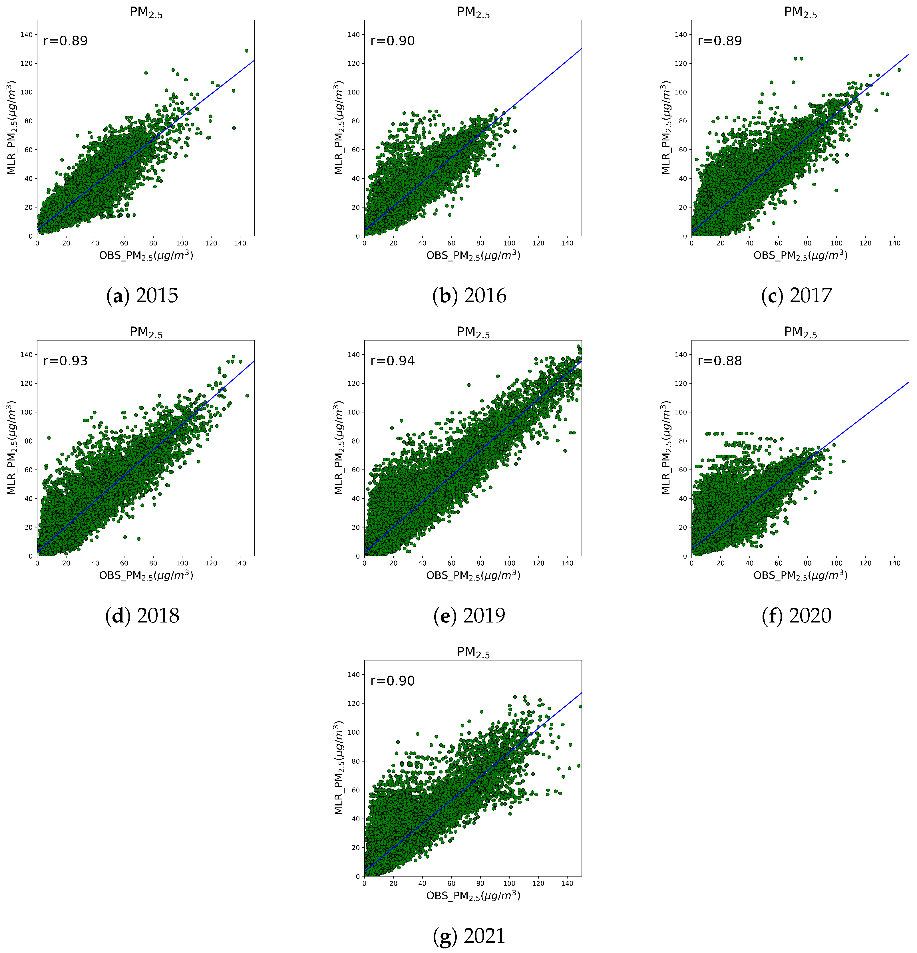
Using the multiple regression equations for the years 2015 to 2021, reanalyzed PM2.5 concentration data were generated. Multiple regression analysis was applied separately for each year depending on the presence or absence of AOD and NDVI. The results of the multiple regression analysis are summarized in Table 5 and Figure 3. Statistical comparisons were made against data from the national automatic air quality monitoring network. The statistical analysis results showed that the R value for PM2.5 ranged from 0.88 to 0.94, the Index of Agreement (IOA) was between 0.93 and 0.97, and the Root Mean Square Error (RMSE) was between 5.52 and 6.90 μ g / m 3 , indicating a very high correlation with the measured values. Additionally, when examining the trends of Mean Bias (MB) and Normalized Mean Bias (NMB), it was found that the model values were variably overestimated or underestimated compared to the measured values in each year. The scatter plots show that the model and measured values are clustered around the trend line with consistent density. As a result, it can be concluded that highly accurate exposure concentration data were generated. However, it can be observed that the spread of the scatter plot from 2019 to 2021 is somewhat more dispersed compared to previous years. The area where the scatter plot spreads is primarily the area where the model tends to overestimate. The reason for this is that the emission data used in this study are based on 2015 emissions, while South Korea’s emissions (CAPSS) have been steadily decreasing since then (https://www.air.go.kr/, accessed on 11 August 2024). As a result, despite applying data assimilation, there is a possibility that the model concentration is overestimated due to the impact of regionally overestimated emissions as the years progress.

4.3. Spatial Distribution of Seasonal and Annual Average PM2.5 Concentrations

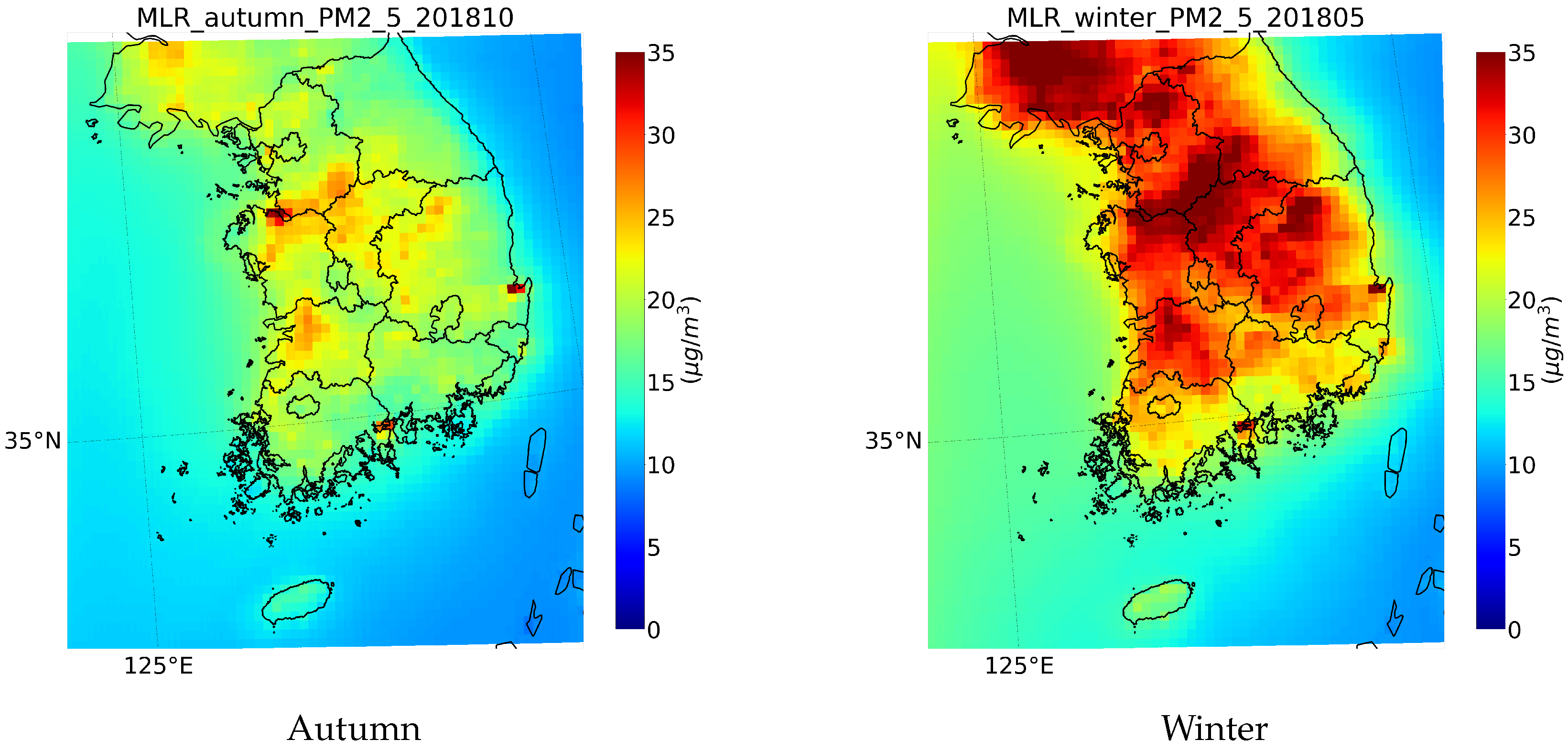
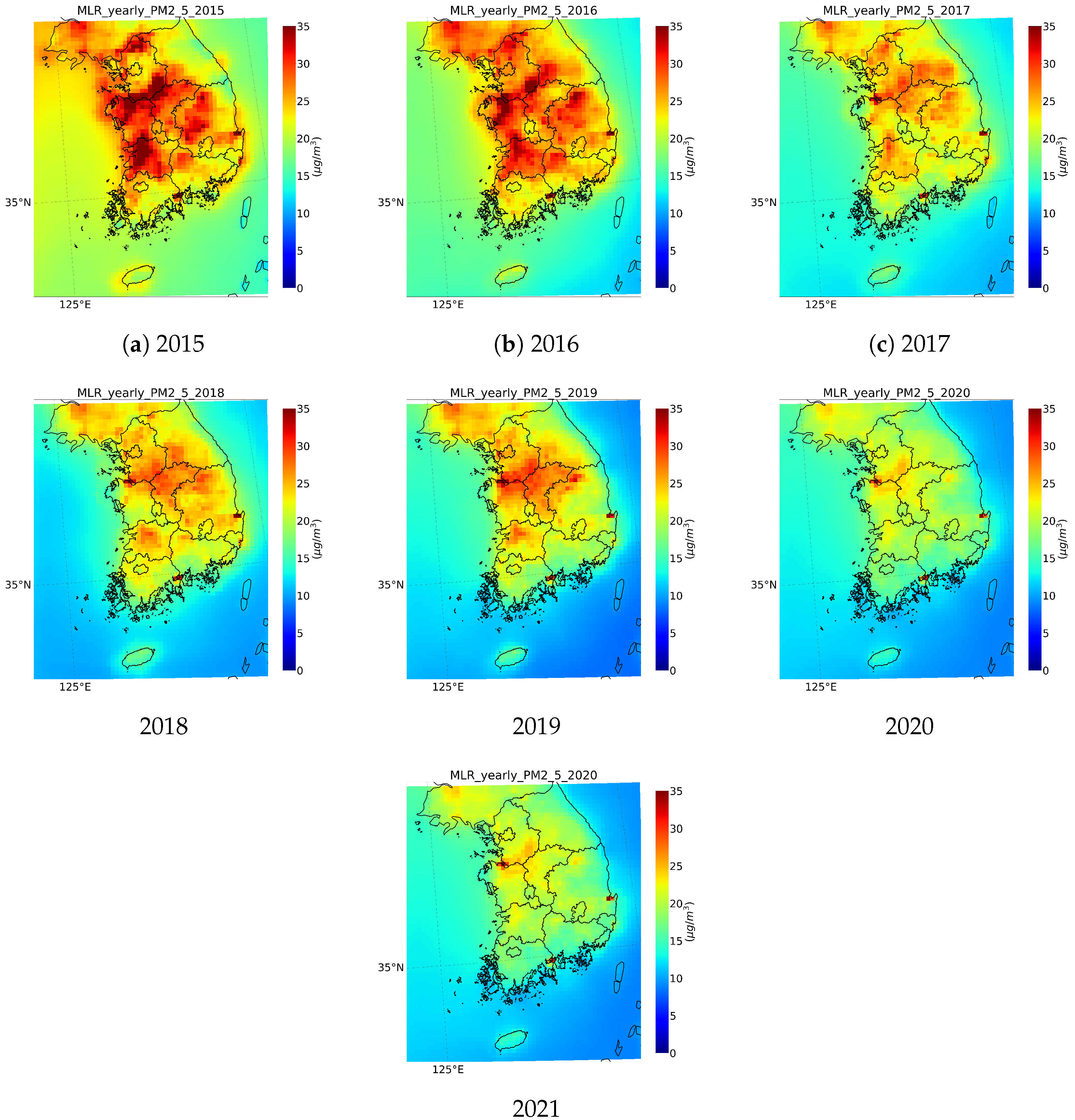
The multiple regression equations derived in this study were applied across South Korea using a 1 km grid to calculate daily average PM2.5 concentrations, which were subsequently used to derive the annual average concentration distribution. Figure 4 and Figure 5 illustrate the spatial distribution of annual average PM2.5 concentrations. The seasonal assessment is a seasonal average from 2015 to 2021. Spring is averaged from March to May, summer from June to August, autumn from September to November, and winter from December, January, and February. Seasonally, PM2.5 concentrations are higher in spring and winter, and spatially, relatively high PM concentrations are found in Gyeonggi-do and Chungcheong-do, which are located outside of Seoul in the Seoul metropolitan area. The high concentration of PM in spring and winter can be attributed to the influence of PM from long-range transport, fuel use, seasonal meteorological effects, and chemical reactions due to the geographical characteristics of Korea (Koo et al., 2012, 2015, 2018) [36,37,38]. Annually, PM2.5 concentrations decreased annually from 2015 to 2018, increased in 2019, then declined again in 2020, likely due to the impact of the COVID-19 pandemic, and increased once more in 2021. Overall, there was a significant reduction in PM2.5 concentrations from 2015 to 2021. Higher PM2.5 concentrations were observed in areas outside Seoul, particularly in Gyeonggi Province and Chungcheong Province, consistent with the distribution observed by the national monitoring network. While satellite data provided a spatial resolution of 1 km and the multiple regression analysis was conducted at this resolution, the overall resolution was largely influenced by the 9 km resolution of the CMAQ and WRF models. It is suggested that increasing the modeling resolution to 3 km or 1 km will be necessary in future studies to achieve truly high-resolution PM concentration estimates.

5. Conclusions

This study presents an approach for estimating high-resolution (1 km) daily PM2.5 exposure concentrations across the Korean Peninsula from 2015 to 2021 by using CMAQ data assimilation, meteorological model data, AOD, and NDVI, integrated through multiple linear regression (MLR). The combination of these various data sources allowed for a more accurate and spatially comprehensive understanding of PM2.5 distributions, particularly in regions where surface observations are sparse or nonexistent. The use of satellite-derived AOD and NDVI data could address limitations typically faced in suburban and rural areas where direct air quality measurements are less available. Through the integration of these datasets, the study was able to fill spatial gaps and generate a more detailed PM2.5 exposure concentrations in the region. The application of MLR ensured that the relationships between environmental variables were captured, further improving the precision of the PM2.5 exposure estimates. Future research will aim to extend the temporal scope. By refining the model and incorporating additional datasets, this approach has the potential to further improve the accuracy of PM2.5 exposure predictions, contributing to better air quality management and public health protection.

Author Contributions

Conceptualization, D.-R.C.; writing—original draft preparation, J.-G.K.; supervision and editing, D.-R.C.; revision and editing, J.-G.K.; software, J.-B.L., J.-Y.L. and J.-H.L.; data curation, H.-Y.Y. All authors have read and agreed to the published version of the manuscript.

Funding

This research was supported by the Korea National Institute of Health (KNIH) research project (No. 2024-ER0606-00) and by the Particulate Matter Management Specialized Graduate Program through the Korea Environmental Industry & Technology Institute (KEITI) funded by the Ministry of the Environment (MOE).

Institutional Review Board Statement

Not applicable.

Informed Consent Statement

Not applicable.

Data Availability Statement

The data presented in this study are available on request from the corresponding author. The data are not publicly available due to privacy.

Conflicts of Interest

The authors declare no conflicts of interest.

References

  1. Pope, C.A., III; Lefler, J.S.; Ezzati, M.; Higbee, J.D.; Marshall, J.D.; Kim, S.Y.; Bechle, M.; Gilliat, K.S.; Vernon, S.E.; Robinson, A.L.; et al. Mortality Risk and Fine Particulate Air Pollution in a Large, Representative Cohort of U.S. Adults. Environ. Health Perspect. 2019, 127, 77007. [Google Scholar] [CrossRef] [PubMed]
  2. World Health Organization. Ambient Air Pollution: A Global Assessment of Exposure and Burden of Disease. 2016. Available online: https://www.who.int/publications/i/item/9789241511353 (accessed on 11 August 2024).
  3. Hwang, M.J.; Cheong, H.K.; Kim, J.H.; Koo, Y.S.; Yun, H.Y. Ambient air quality and subjective stress level using Community Health Survey data in Korea. Epidemiol. Health 2018, 40, 1–9. [Google Scholar] [CrossRef] [PubMed]
  4. Kim, J.H.; Oh, I.H.; Park, J.H.; Cheong, H.K. Premature Deaths Attributable to Long-term Exposure to Ambient Fine Particulate Matter in the Republic of Korea. J. Korean Med. Scil. Atmos. Environ. 2018, 33, e251. [Google Scholar] [CrossRef]
  5. Lim, H.; Kown, H.J.; Lim, J.A.; Choi, J.H.; Ha, M.; Hwang, S.S.; Choi, W.J. Short-term Effect of Fine Particulate Matter on Children’s Hospital Admissions and Emergency Department Visits for Asthma: A Systematic Review and Meta-analysis. J. Prev. Med. Public Health 2016, 49, 205–219. [Google Scholar] [CrossRef] [PubMed]
  6. Kim, H.; Kim, H.; Lee, J.T. Effect of air pollutant emission reduction policies on hospital visits for asthma in Seoul, Korea; Quasi-experimental study. Environ. Int. 2019, 132, 104954. [Google Scholar] [CrossRef]
  7. Beckerman, B.S.; Jerrett, M.; Martin, R.V.; Donkelaar, A.V.; Ross, Z.; Burnett, R.T. Application of the deletion substitution addition algorithm to selecting land use regression models for interpolating air pollution measurements in California. Atmos. Environ. 2013, 77, 142–149. [Google Scholar] [CrossRef]
  8. Li, L.; Zhang, J.; Meng, X.; Fang, Y.; Ge, Y.; Wang, J. Estimation of PM2.5 concentrations at a high spatiotemporal resolution using constrained mixed-effect bagging models with MAIAC aerosol optical depth. Remote Sens. Environ. 2018, 217, 573–586. [Google Scholar] [CrossRef]
  9. Chamependal, A.; Kanevski, M.; Huguenot, P.E. Air Pollution Mapping Using Nonlinear Land Use Regression Models. In Computational Science and Its Applications—ICCSA 2014; Lecutre Notes in Computer Science; Springer: Cham, Switzerland, 2014; pp. 682–690. [Google Scholar]
  10. Beloconia, A.; Chrysoulakis, N.; Lyapustin, A.; Utzinger, J.; Vounatsou, P. Bayesian geostatistical modelling of PM10 and PM2.5 surface level concentrations in Europe using high resolution satellite derived products. Environ. Int. 2018, 121, 57–70. [Google Scholar] [CrossRef]
  11. Stafoggia, M.; Bellander, T.; Bucci, S.; Davoli, M.; de Hoogh, K.; de’ Donato, F.; Gariazzo, C.; Lyapustin, A.; Michelozzi, P.; Renzi, M.; et al. Estimation of daily PM10 and PM2.5 concentrations in Italy, 2013-2015, using a spatiotemporal land use random-forest model. Environ. Int. 2019, 124, 170–179. [Google Scholar] [CrossRef]
  12. Ndiaye, A.; Shen, Y.; Kyriakou, K.; Karssenberg, D.; Schimitz, O.; Flukiger, B.; Hoogh, K.; Hoek, G. Hourly land-use regression modeling for NO2 and PM2.5 in the Netherlands. Environ. Res. 2024, 256, 119233. [Google Scholar] [CrossRef]
  13. Chen, G.; Wang, Y.; Li, S.; Cao, W.; Ren, H.; Knibbs, L.D.; Abramson, M.J.; Guo, Y. Spatiotemporal patterns of PM10 concentrations over China during 2005–2016 A satellite-based estimation using the random forests approach. Environ. Pollut. 2018, 242, 605–613. [Google Scholar] [CrossRef]
  14. Xue, T.; Zheng, Y.; Tong, D.; Zheng, B.; Li, X.; Zhu, T.; Zhang, Q. Spatiotemporal continuous estimates of PM2.5 concentrations in China, 2000-2016:A machine learning method with inputs from satellites, chemical transport model, and ground observations. Environ. Int. 2022, 123, 345–357. [Google Scholar] [CrossRef] [PubMed]
  15. Jin, X.; Fiore, A.M.; Curci, G.; Lyapustin, A.; Civerolo, K.; Ku, M.; van Donkelaar, A.; Martin, R.V. Assessing uncertainties of a geophysical approach to estimate surface fine particulate matter distributions from satellite-observed aerosol optical depth. Atmos. Chem. Phys. 2019, 19, 295–313. [Google Scholar] [CrossRef]
  16. Wang, F.; Yao, S.; Luo, H.; Huang, B. Estimating High-Resolution PM2.5 Concentrations by Fusing Satellite AOD and Smartphone Photographs Using a Convolutional Neural Network and Ensemble Learning. Remote Sens. 2022, 14, 1515. [Google Scholar] [CrossRef]
  17. Park, S.H.; Lee, J.H.; Im, J.H.; Song, C.K.; Choi, M.J.; Kim, J.; Lee, S.G.; Park, R.J.; Kim, S.M.; Yoon, J.M.; et al. Estimation of spatially continuous daytime particulate matter concentrations under all sky conditions through the synergistic use of satellite-based AOD and numerical models. Sci. Total. Environ. 2020, 713, 136516. [Google Scholar] [CrossRef] [PubMed]
  18. Lee, C.S.; Lee, K.H.; Kim, S.M.; Yu, J.H.; Jeong, S.T.; Yeom, J.M. Hourly Ground-Level PM2.5 Estimation Using Geostationary Satellite and Reanalysis Data via Deep Learning. Remote Sens. 2021, 13, 2121. [Google Scholar] [CrossRef]
  19. Lee, S.H.; Park, S.H.; Lee, M.I.; Kim, G.H.; Im, J.H.; Song, C.K. Air Quality Forecasts Improved by Combining Data Assimilation and Machine Learning with Satellite AOD. Geophys. Res. Lett. 2022, 49, e2021GL096066. [Google Scholar] [CrossRef]
  20. Tang, B.; Stanier, C.O.; Carmichael, G.R.; Gao, M. Ozone, nitrogen dioxide, and PM2.5 estimation from observation-model machine learning fusion over S. Korea: Influence of observation density, chemical transport model resolution, and geostationary remotely sensed AOD. Atmosphere 2024, 331, 120603. [Google Scholar] [CrossRef]
  21. Cho, S.Y.; Park, H.Y.; Son, J.S.; Chang, L.S. Development of the Global to Mesoscale Air Quality Forecast and Analysis System (GMAF) and Its Application to PM2.5 Forecast in Korea. Atmosphere 2021, 12, 411. [Google Scholar] [CrossRef]
  22. Lyapustin, A.; Martonchik, J.; Wang, Y.; Laszlo, I.; Korkin, S. Multiangle implementation of atmospheric correction (MAIAC): 1. Radiative transfer basis and look-up tables. J. Geophys. Res. Atmos. 2011, 116, D03210. [Google Scholar] [CrossRef]
  23. Lyapustin, A.; Wang, Y. MCD19A2 V006 [Data set]. MODIS/Terra+Aqua Land Aerosol Optical Depth Daily L2G Global 1km SIN Grid. In NASA EOSDIS Land Processes DAAC; NASA: Washington, DC, USA, 2018. [Google Scholar] [CrossRef]
  24. Koo, Y.S.; Choi, D.R.; Yun, H.Y.; Yun, G.W.; Lee, J.B. A Development of PM Concentration Reanalysis Method using CMAQ with Surface Data Assimilation and MAIAC AOD in Korea. Korean J. Atmos. Environ. 2020, 16, 558–573. [Google Scholar] [CrossRef]
  25. Choi, D.R.; Yun, H.Y.; Koo, Y.S. A Development of Air Quality Forecasting System with Data Assimilation using Surface Measurements in East Asia. JKOSAE 2019, 35, 60–85. [Google Scholar] [CrossRef]
  26. Skamarock, W.C.; Klemp, J.B. A time-split nonhydrostatc atmospheric model for weather reasearch and forecasting applications. J. Comput. Phys. 2008, 227, 3465–3485. [Google Scholar] [CrossRef]
  27. Borge, R.; Lopez, J.; Lumbereas, J.; Narros, A.; Rodriguez, E. Influence of boundary conditions on CMAQ simulations over the Iberian Peninsula. Atmos. Environ. 2010, 44, 2681–2695. [Google Scholar] [CrossRef]
  28. Byun, D.W.; Ching, J.K.S. Science Algorithms of the EPA Models-3 Community Multiscale Air Quality (CMAQ) Modeling System; EPA: Washington, DC, USA, 1998.
  29. Byun, D.W.; Schere, K.L. Review of the governing equations, computational algorithm and other components of the Models-3 Community Multi-scale Air Quality (CMAQ) modeling system. ASME 2006, 59, 51–77. [Google Scholar]
  30. Woo, J.H.; Kim, Y.H.; Kim, H.K.; Choi, K.C.; Eum, J.H.; Lee, J.B.; Lim, J.H.; Kim, J.Y.; Seong, M.A. Development of the CREATE Inventory in Support of Integrated Climate and Air Quality Modeling for Asia. Sustainability 2020, 12, 7930. [Google Scholar] [CrossRef]
  31. Lee, D.; Lee, Y.; Jang, K.; Yoo, C.; Kang, K.; Lee, J.; Jung, S.; Park, J.; Lee, S.; Han, J.; et al. Korean National Emissions Inventory System and 2007 Air Pollutant Emissions. Asian J. Atmos. Environ. 2011, 5, 278–291. [Google Scholar] [CrossRef]
  32. Cressman, G.P. An Operational Objective Analysis System, An Operational Objective Analysis System. Mon. Weather. Rev. 1959, 87, 364–374. [Google Scholar] [CrossRef]
  33. Pun, K.; Seigneur, C. Using CMAQ interpolate among CASTNET measurements. In Proceedings of the CMAS Conference, Chapel Hill, NC, USA, 16–18 October 2006; Available online: https://www.cmascenter.org/conference/2006/abstracts/pun_session7.pdf (accessed on 11 August 2024).
  34. Cohen, J. The Earth is Round (p < .05). Am. Psychol. 1994, 49, 997–1003. [Google Scholar]
  35. Ioannidis, J.P.A. Why most published research findings are false. Remote Sens. PLoS Med. 2005, 2, e124. [Google Scholar] [CrossRef]
  36. Koo, Y.S.; Kim, S.T.; Cho, J.S.; Jang, Y.K. Performance evaluation of the updated air quality forecasting system for Seoul predicting PM10. Atmos. Environ. 2012, 58, 56–69. [Google Scholar] [CrossRef]
  37. Koo, Y.S.; Choi, D.R.; Kwon, H.Y.; Jang, Y.K.; Han, J.S. Improvement of PM10 prediction in East Asia using inverse modeling. Atmos. Environ. 2015, 106, 318–328. [Google Scholar] [CrossRef]
  38. Koo, Y.S.; Yun, H.Y.; Choi, D.R.; Han, J.S.; Lee, J.B.; Lim, Y.J. An analysis of chemical and meteorological characteristics of haze events in the Seoul metropolitan area during January 12–18, 2013. Atmos. Environ. 2018, 178, 87–100. [Google Scholar] [CrossRef]
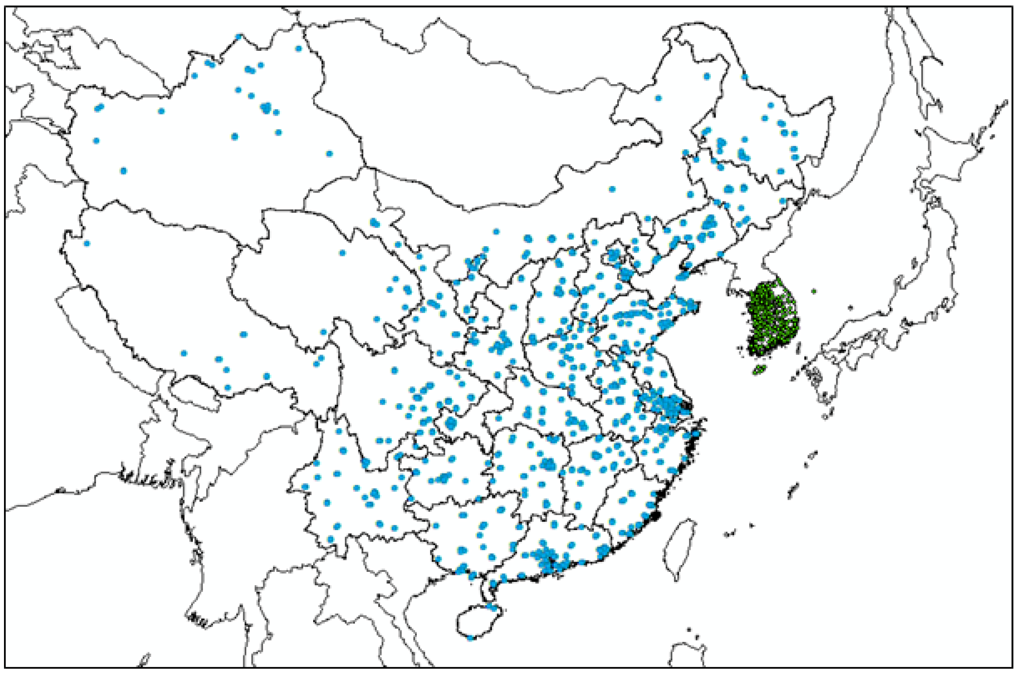
Figure 1. Locations of ambient air quality monitoring stations in the region of China and Korea (blue dots: china monitoring stations, green dots: south korea monitoring stations).
Atmosphere 15 01152 g001
Figure 2. Modeling domain (Domain 1: East Asia, Domain 2: South Korea).
Atmosphere 15 01152 g002
Figure 3. Scatter plots of MLRs with observations for 2015–2021.
Atmosphere 15 01152 g003
Figure 4. Reanalyzed average seasonal PM2.5 distribution in 2015–2021.
Atmosphere 15 01152 g004aAtmosphere 15 01152 g004b
Figure 5. Reanalyzed annual PM2.5 distribution in 2015–2021.
Atmosphere 15 01152 g005
Table 1. Predictor variables used in MLR.
Satellite DataDescriptionCMAQ and WRF Model DataDescription
MODIS AODMAIAC MCD19 AODM_PM10assimilated PM10
MODIS NDVIMAIAC MOD13 NDVIM_PM2.5assimilated PM2.5
M_TEMPWRF prediction
M_PLBWRF prediction
M_RHWRF prediction
M_WSWRF prediction
M_PRSFCWRF prediction
Table 2. The p-values of predictors with target PM2.5.
Predictor2015201620172018201920202021
M_PM2.50.0000.0000.0000.0000.0000.0000.000
M_PBL0.0000.0000.0000.0000.0000.0000.000
M_WS0.0000.0000.0000.0000.1340.2480.000
M_SPRES0.0000.0000.0000.0000.0000.0000.000
M_TEMP0.0000.0730.0000.0000.0000.0030.009
M_RH0.0000.1560.0000.0000.4150.0000.000
AOD0.0000.0000.0000.0000.0000.0000.000
NDVI0.0080.0000.0000.0150.0000.0000.000
Table 3. MLR equations with various conditions for 2015–2021 with AOD and NDVI.
TypeYearMLR Equations
MLR (With
AOD and NDVI)
2015 M L R _ P M 2.5 = 31.5201 + 1.0405 × M _ P M 2.5 0.0019 × M _ P B L + 0.9823 × M _ W S 0.0381 × M _ S P R E S + 0.1635 × M _ T E M P + 0.0370 × M _ R H 3.3988 × A O D 1.0346 × N D V I
2016 M L R _ P M 2.5 = 43.3142 + 0.9995 × M _ P M 2.5 0.0013 × M _ P B L + 0.5618 × M _ W S 0.0467 × M _ S P R E S + 0.0125 × M _ T E M P + 0.0057 × M _ R H + 2.6268 × A O D + 2.7182 × N D V I
2017 M L R _ P M 2.5 = 47.1088 + 0.9524 × M _ P M 2.5 0.0090 × M _ P B L + 0.1427 × M _ W S 0.0495 × M _ S P R E S 0.0491 × M _ T E M P + 0.0155 × M _ R H + 5.3998 × A O D + 2.6348 × N D V I
2018 M L R _ P M 2.5 = 62.7106 + 0.9504 × M _ P M 2.5 0.0041 × M _ P B L + 0.1976 × M _ W S 0.0625 × M _ S P R E S 0.0218 × M _ T E M P + 0.0303 × M _ R H + 5.5989 × A O D 0.6427 × N D V I
2019 M L R _ P M 2.5 = 58.9434 + 0.9744 × M _ P M 2.5 0.0019 × M _ P B L + 0.0495 × M _ W S 0.0585 × M _ S P R E S 0.0693 × M _ T E M P + 0.0018 × M _ R H + 7.3718 × A O D 1.0368 × N D V I
2020 M L R _ P M 2.5 = 45.0425 + 0.8426 × M _ P M 2.5 0.0033 × M _ P B L + 0.0294 × M _ W S 0.04340 × M _ S P R E S 0.0122 × M _ T E M P + 0.0295 × M _ R H + 7.0544 × A O D 0.8609 × N D V I
2021 M L R _ P M 2.5 = 46.0479 + 0.9234 × M _ P M 2.5 0.0049 × M _ P B L + 0.5137 × M _ W S 0.0448 × M _ S P R E S + 0.0126 × M _ T E M P 0.0238 × M _ R H + 10.4224 × A O D 1.6674 × N D V I
Table 4. MLR equations with various conditions for 2015–2021 without AOD and NDVI.
TypeYearMLR Equations
MLR (Without
AOD and NDVI)
2015 M L R _ P M 2.5 = 30.9761 + 1.0763 × M _ P M 2.5 0.0016 × M _ P B L + 1.0080 × M _ W S 0.0386 × M _ S P R E S + 0.1850 × M _ T E M P + 0.0409 × M _ R H
2016 M L R _ P M 2.5 = 48.5012 + 1.0179 × M _ P M 2.5 0.0013 × M _ P B L + 0.5906 × M _ W S 0.0515 × M _ S P R E S + 0.0261 × M _ T E M P + 0.0108 × M _ R H
2017 M L R _ P M 2.5 = 57.1602 + 0.9851 × M _ P M 2.5 + 0.0005 × M _ P B L + 0.2055 × M _ W S 0.0591 × M _ S P R E S + 0.0110 × M _ T E M P + 0.0218 × M _ R H
2018 M L R _ P M 2.5 = 59.5261 + 1.0048 × M _ P M 2.5 0.0031 × M _ P B L + 0.1911 × M _ W S 0.0610 × M _ S P R E S 0.0114 × M _ T E M P + 0.0453 × M _ R H
2019 M L R _ P M 2.5 = 57.0963 + 1.0274 × M _ P M 2.5 0.0012 × M _ P B L 0.0178 × M _ W S 0.0576 × M _ S P R E S 0.0375 × M _ T E M P + 0.0102 × M _ R H
2020 M L R _ P M 2.5 = 43.7489 + 0.8945 × M _ P M 2.5 0.0027 × M _ P B L + 0.0886 × M _ W S 0.0439 × M _ S P R E S + 0.0382 × M _ T E M P + 0.0373 × M _ R H
2021 M L R _ P M 2.5 = 39.8673 + 0.9920 × M _ P M 2.5 0.0041 × M _ P B L + 0.4320 × M _ W S 0.0400 × M _ S P R E S + 0.0354 × M _ T E M P 0.0016 × M _ R H
Table 5. MLR performance summary for 2015–2021.
YearRR2IOARMSEMBNMB
20150.890.790.946.58−1.16−4.54
20160.900.820.955.66−0.40−1.54
20170.890.790.946.90−1.78−7.13
20180.930.870.965.520.140.62
20190.940.880.975.73−0.23−1.01
20200.880.770.935.680.713.80
20210.900.820.955.600.281.60
Disclaimer/Publisher’s Note: The statements, opinions and data contained in all publications are solely those of the individual author(s) and contributor(s) and not of MDPI and/or the editor(s). MDPI and/or the editor(s) disclaim responsibility for any injury to people or property resulting from any ideas, methods, instructions or products referred to in the content.