Review: Fractal Geometry in Precipitation

Abstract

Rainfall, or more generally the precipitation process (flux), is a clear example of chaotic variables resulting from a highly nonlinear dynamical system, the atmosphere, which is represented by a set of physical equations such as the Navier–Stokes equations, energy balances, and the hydrological cycle, among others. As a generalization of the Euclidean (ordinary) measurements, chaotic solutions of these equations are characterized by fractal indices, that is, non-integer values that represent the complexity of variables like the rainfall. However, observed precipitation is measured as an aggregate variable over time; thus, a physical analysis of observed fluxes is very limited. Consequently, this review aims to go through the different approaches used to identify and analyze the complexity of observed precipitation, taking advantage of its geometry footprint. To address the review, it ranges from classical perspectives of fractal-based techniques to new perspectives at temporal and spatial scales as well as for the classification of climatic features, including the monofractal dimension, multifractal approaches, Hurst exponent, Shannon entropy, and time-scaling in intensity–duration–frequency curves.

1. Introduction

1.1. Geometrical Motivation

Observed precipitation is a chaotic variable that usually is represented by aggregated values in time series instead of physical fluxes as directly simulated by numerical weather prediction models [1]. Climate variability of precipitation is defined to range from the subseasonal and seasonal phases [2,3,4] to multi-decadal and centennial fluctuations [5,6,7,8,9]. A large number of its different variability modes presents self-similarity at most time scales, which is a key in the climatic characterization of its chaotic-related complexity [10,11,12]. Considering this idea, climate change (signal) detection and a variability analysis can consider other measurements beyond the commonly used techniques such as average temporal statistics, spatial atmospheric patterns, and compound extreme events [13,14,15,16]. This review aims to identify both classical and emergent geometrical techniques used in the analysis of climate complexity of precipitation. Therefore, a brief reminder of basic ideas of geometry is required to understand the subjacent motivation and most of the approaches reviewed here.

One of the most important concepts in geometry is the measurement or mathematical measure, which is a set of techniques that depends on the discipline considered [17,18]. A measure is a function, $\mu :s\to \mathbb{R}$, that assigns (scalar) values in $\mathbb{R}$ to a subset, $s\subset S$, of elements of a system, $S$, or to some of its states (also known as properties, observables, or magnitudes). According to the theory of physical measurement, it is usual to distinguish between intensive (e.g., density, pressure, wind velocity, friction, temperature, viscosity) and extensive (e.g., mass, energy, duration, snow depth, precipitation amount, additive entropy) measurements [19,20]. In measure theory of geometry, the ‘measure’ term is just reserved for the extensive properties of sets, only assigning values on positive real numbers. The most elementary measure of a set is that which relates to its ‘size’, that is, length, area, and volume, as the dimension $d\in \mathbb{N}$ is increasing from $d=1$ in lengths to $d=3$ in volumes, passing through d = 2 for surfaces, and the measure $M$ is increasing as the power law $M\propto L^d$ of the representative length $L$.

In the case of precipitation, one can enumerate a large set of different measurements: the total amount or accumulation, precipitation event duration, wet/dry spell lengths, and drop/hail size, among others [21,22]. Moreover, intensive measures of precipitation could be, for instance, rainfall intensity and drought severity indicators [14,16,23].

Paradoxically, some natural features cannot be described using ‘natural dimensions’ (i.e., positive integer numbers) but require using new techniques such as the fractal theory [1,14,24,25]. The word “fractal” was presented in [26,27] to bring together a kind of objects that have played a historical role in mathematical development in the last third of the past century. The regular geometric shapes and structures of Euclid and their natural dimensions give way to new forms, complex, but underlying a scalar regularity with fractional dimensions.

1.2. Fractal Measure Background

The concept of fractal is used to designate objects that are too irregular to be described according to Euclidean geometry, but which are invariant via a change in scale. Fractal geometry [28,29] is an extension of classical geometry and encompasses the description, classification, and analysis of geometrically “complicated” subspaces. Generally, the structure and organization of a fractal set do not make it possible to specify where—in plain language—each point that composes it is located. Therefore, some relationship must be defined between the various structures observed in it for various levels of resolution. This relationship is formulated quantitatively via the concept of the fractal dimension, which describes the scalar behavior of fractal structures [24,25].

As with fractal objects, scale-invariant systems and processes do not have a particular scale that is specific to them. Accordingly, a fractal process is one in which the same elementary action occurs at different scales, i.e., in which a part reproduces the whole. For the range of scales analyzed, the process statistics follow potential laws characterized by their exponents. The relationship between the statistics for the different scales will simply consist of scale ratios.

Unlike the Euclidean dimensions, which are always non-negative integers (0 for a point, 1 for a line, 2 for a plane, 3 for a three-dimensional space, etc.), fractal dimensions have a more general non-negative real value, which exceeds the topological dimension. To obtain a clearer picture of this, let us suppose a point moving on a plane describing a Brownian motion, i.e., a random motion tending to gradually complete or fill the plane [30]. At the beginning, its dimension will be 0, but at the same instant in which it begins to describe this movement, its fractal dimension will become 1, and immediately after, it will begin to increase decimals, but without reaching two, since it will not complete this plane.

The postulates of fractal geometry have been used in the geographic discipline for more than three decades. It was introduced to measure the length of coastlines of the British Isles [31], and subsequently its use has spread prolifically to a multitude of studies in surveying. Some mathematical algorithms are now available to calculate the fractal dimension for linear and area entities. Indeed, not all geographic patterns are fractal at every scale. While the nature of some geographical multifractal phenomena has been well explored, it remains to be determined why certain types of terrain align better with fractal geometry than others.

Since the idea of fractal objects was introduced to measure shoreline length at certain locations, this kind of analysis has been highly applied to several topographic studies. One of the possible applications has been focused on measuring and characterizing irregular linear features such as coastlines, to describe and characterize landforms, and to statistically regionalize spaces according to relief shape. However, not all these elements are fractal at all the studied scales. A fractal analysis can also be used to produce terrain simulations with a known dimension. Other applications focus on understanding the different geomorphological processes involved [32].

Thus, the problems of estimating area, length, and point features are increasingly promoted largely by the growing interest in digital capture, processing, and storage of geographically referenced data. Therefore, numerous drawbacks appear when obtaining composites of satellite images or aerial photographs that have been taken at different altitudes or with different resolution, and for which it becomes necessary to implement mathematical models around a Geographic Information System (GIS) in which fractals actively intervene [33].

In hydrological basins, as an applied example, the most important principles of fractal objects (such as self-similarity and self-affinity) are reliably reproduced. Thus, numerous elements such as the length of the river network, the number of branches, the bifurcation coefficient, the density of branches per drainage unit, and the perimeter and area of the basin itself, among others, can be treated as applications in fractal mathematical studies. The results obtained provide information on the knowledge of the hydrological characteristics of the area in question [34]. The works that deal with the precise measurement of the length of coasts are the most abundant studies, yielding interesting results such as that the length of a particular coast will vary depending on the fractal dimension of the same, considering the measurement of the same in terms of mapping at different scales [35,36].

As can be deduced, the conceptual environment surrounding fractals is closely related to the spatial concept of scale, fundamental in geography, since it is often a matter of both data and information integration in a multiscalar way. The high access to GIS has enabled an adequate environment that allows re-scaling data prior to the consequent integration of the data into the system. However, the challenges to understand patterns of the spatial variation of the information itself are surpassed by the scarcity of suitable tools because the nature of the spatial variation of the information of interest is not always well analyzed and understood. Spatial patterns are modeled using geostatistical approaches that provide the possibility of re-scaling the data (such as spatial interpolation multiple regression models). These types of regularizations provide information that can often describe the data better than the data itself [37], as is the case in many climate models and climate and weather reanalysis grids.

Climate studies have also applied the fractal analysis methodology, since some of its variables (e.g., pressure, precipitation, temperature, and wind) show a fractal behavior [38]. From the data series of the previously mentioned variables and their monthly and seasonal variability, it is possible to detect how regional climate models are not able to predict the local climate on a seasonal scale, since they only work with averaged quantities. Thus, interesting facts appear such as that, in regions like India, rainfall during the southwest monsoon is affected by the variability of temperature and pressure of the previous winter. Other fractal-based prediction indices are more reliable since they consider more climatic dynamics [39,40].

The analysis of rescaled ranges of annual mean temperatures at different meteorological stations in Hungary has shown that this variable follows a fractal behavior, both on time scales ranging from a few years to approaching the millennium [41]. These analyses could indicate that the existence of this fractal behavior is a characteristic of climate change during the study period. Variations of the fractal dimension values linked to the used time scale would show different behaviors at different scales.

In the same vein is that purely mathematical fractal theories playing an important role in climate modeling has become evident not only on a regional scale, as explained above, but also on a global scale [42]. The factors that most obviously affect planetary temperatures (response to solar cycles, large volcanic eruptions, increasing concentrations of greenhouse gasses and aerosols in the atmosphere) fit appropriately with those predicted using models created from introducing fractal theories.

However, other findings have appeared that propose new analysis processes to discriminate between climate temporal behavior data generated using climate models and observations from instrumental weather stations. These approaches combine monitoring of actual and model-generated data streams and a fractal data analysis to identify differences in the correlation between observed and model-predicted series. Thus, from this comparison, it is concluded that the fractal approach allows us to correctly discriminate the data, from which it follows that there is still the chance to improve climate change models supported by fractal theories [43,44].

In paleoclimatology, the study of soundings or “cores” extracted from glaciers has a key role in determining past climate conditions [45,46]. The analysis of the air bubbles confined in the ice reveals the chemical composition of the atmosphere at the time when the bubble was imprisoned, as well as the conditions under which the ice was formed, based on its level of compaction. The latter is determined by studying the conductivity of the ice at a known electrical impulse, and it has been found to be scale-invariant over three different orders of magnitude in the depth of the ice core. This experiment carried out in Antarctica, from an ice core 3190 m thick, makes it possible to establish climatic connections between the past 740,000 years and the fractal analysis, to provide information on the occurrence of glacial ages [47]. Previous studies have linked Antarctic ice core information with historical climate data obtained from sediments in the deep ocean [48,49]. Like a geometrical footprint of complex dynamical systems, the fractal approach provides evidence that relates climate data from geographically distant locations, such as in Central Europe [41] and the Kamchatka Peninsula, over the last 10,000 years [50], or, on a shorter time scale, from sediment records in alluvial plains in the Mediterranean basin [51].

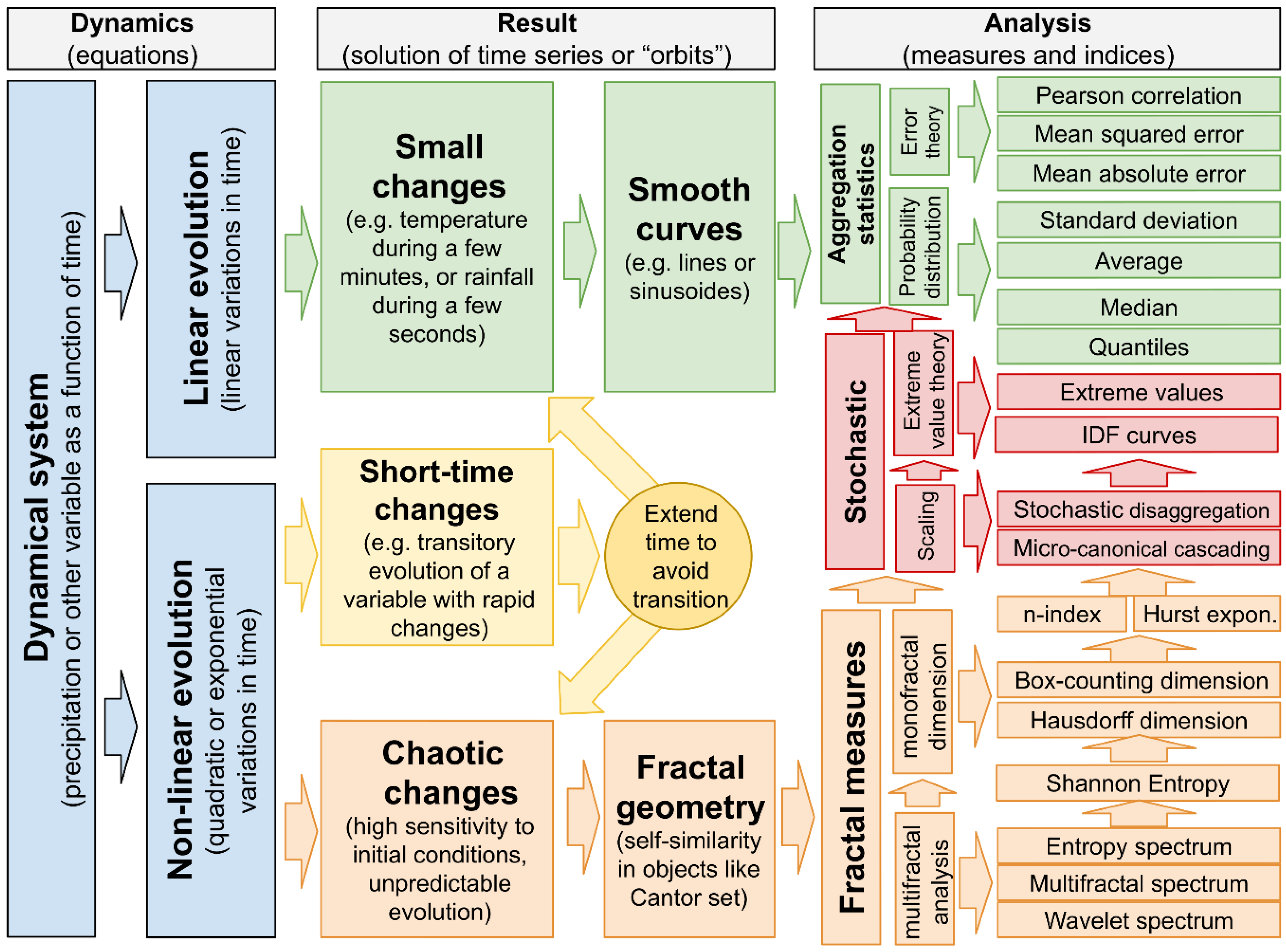
1.3. Geometry in Dynamical Systems

The atmosphere is a highly nonlinear dynamical system, governed by physical equations such as the Navier–Stokes equations, energy balances, and the hydrological cycle, among others. These well-known physical concepts are deeply studied in differential and computational geometry. A brief review of some basic definitions is presented here.

Dynamical system. As a starting point, most complex systems are easily addressable under discrete geometry. Let a system, $S=(X,f)$, be defined as a set, $X$, of elements with characteristics or states and some law $f$ that describes a (natural or not) behavior. Then, a dynamical system is that whose behavior depends on a variable assimilable to the time [52,53,54]. In the case of a discrete time (i.e., a natural number), the law is a continuous function, $f:\mathbb{N}\to \mathbb{R}$, that determines the temporal evolution of the values of a state variable of the system [52,54]. For example, in the study on populations of biological species, the abundance of individuals $x$ in the time $n\in \mathbb{N}$ can be simplified using the logistic map

$$x_n=r·x_{n-1}·(1-x_{n-1}),$$

where $r$ is a parameter that indicates the relative reproduction rate compared to the competition rate [55]. Similarly, continuous variables like the wind components $\left(u\right(t),v(t\left)\right)$ of a frontal system (e.g., cold front) are also governed by an evolution law but with a real time, $t\in \mathbb{R}$. From Newton’s second law, the (differential) equations of the simplest or geostrophic wind are as follows [56,57]:

$$\frac{du\left(t\right)}{dt}=F_u(t)=-f_x+f_C·v(t),$$

$$\frac{dv\left(t\right)}{dt}=F_v(t)=-f_x-f_C·u(t)$$

where $f_C$ is the Coriolis parameter and $f_x$:=$\left(f_x,f_y\right)\equiv \frac{1}{\rho }\left(\frac{\partial P}{\partial x},\frac{\partial P}{\partial y}\right)$is the acceleration caused by the gradient of the pressure $P$ at the position $\left(x,y\right)\in {\mathbb{R}}^2$ for a fluid with density $\rho$. Under a computational perspective, differential equations can be expressed in terms of finite differences according to a discretization of the time $t\approx n\delta$for some small-time lapse $\delta >0$ and $n\in \mathbb{N}$ [58]. For example, as the u-component of wind is now $u\left(t\right)\equiv u\left(n\delta \right)\equiv u_n$, then

$$\frac{du\left(n\right)}{dt}\approx \frac{u_n-u_{n-1}}{\delta }=F_u(n)\Rightarrow u_n=\delta F_u(n)+u_{n-1}$$

Therefore, differential geometry applied to atmospheric sciences can be computationally discretized and most of the properties are then inferred.

Nonlinearity and chaos. A dynamical system is nonlinear if the governance law is not simply linear with respect to the temporal variable [52,59]. For example, in the case of the logistic map and geostrophic wind, they have quadratic terms that provide a high complexity in their behavior. Solutions of the dynamical equations are known as orbits or paths, which are grouped in a phase space of positions ($u\left(n\right)$) and momenta ($du\left(n\right)/dt$) according to the symplectic geometry [60]. After a sufficient transitory time, stable solutions are attractors or attractive regions of the phase space, because the evolution of a given variable tends to approach these regions. In some cases, highly nonlinear systems present unpredictable solutions for a certain transitory time, due to a high transitivity and sensitivity to initial conditions. The scientific community defines these cases as chaotic solutions or simply chaos [61]. A remarkable consequence of the chaotic systems is that phase space presents strange attractors, characterized by fractal measures [59,62]. The Lorenz fractal is a very popular example derived from simplified Navier–Stokes equations [63].

Self-similarity. Among others, fractals have a remarkable feature of being similar to themselves when two or more different scales are compared, like a homothety symmetry (e.g., similar triangles). This surprising character allows the use of stochastic cascading, spatial or temporal scaling methods, and the disaggregation of time series or spatial distributions [1,64].

Quasi-oscillations. In a chaotic dynamical system such as the atmosphere, most variables (precipitation, temperature, humidity, and pressure, among others) present a large number of different modes in both spatial and temporal variability. This is a set of diverse amplitudes of anomalies, with more regular or periodic (predictable) components and other unpredictable phases. These modes of variability are known as quasi-periodic oscillations or simply quasi-oscillations [2,12]. There exists a large number of techniques that aim to determine the periodicity level of quasi-oscillations, like the fast Fourier transformation and the wavelet analysis, which decompose temporal variability in a set of period oscillations [65]. Assuming some appropriate technique to model orbits without overfitting, residual unexplained variance would be a ‘pure chaotic’ component of the particular time series analyzed. In this case, other approaches (e.g., based on random probability distributions) are commonly used.

1.4. Structure of the Review

After this introductory section, the review is structured in two main parts: Section 2 is focused on classical perspectives of fractal measures used in an analysis of time series of precipitation, including monofractal and multifractal approaches, temporal concentration indices, and other measures such as the Shannon entropy, Hurst exponent, and IDF curves. On the other hand, Section 3 explores new perspectives of precipitation fractality at temporal and spatial scales as well as for the classification of climatic features. Finally, Section 4 summarizes the main conclusions of the review.

2. Classical Perspectives of Precipitation Fractality

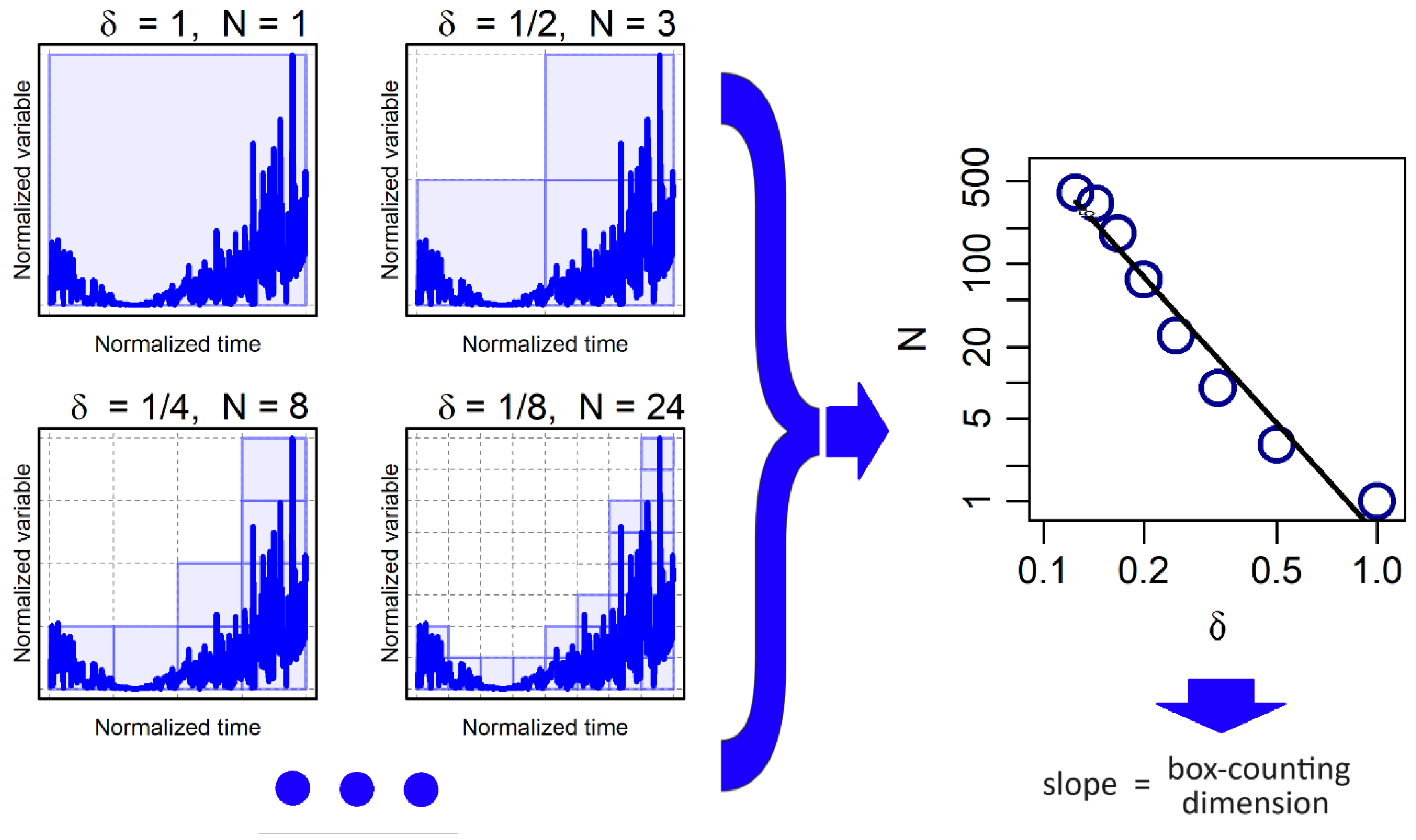
2.1. Monofractal Dimension

As mentioned above, non-integer or fractional dimensions are naturally found for nonsmooth geometries with self-similarity at different scales, which is usually assumed as a unique behavior (so-called “monofractal”). For objects constructed using iterative processes (e.g., Cantor set, Sierpinski triangle, and Koch curve), it is possible to define the Hausdorff–Besicovitch dimension D_H by using the numbed N of self-similar fragments, which are rescaled copies (homothety) of the original object by applying a scaling factor of $1/S$. Thus, it is

$$D_H=\frac{\mathrm{l}\mathrm{o}\mathrm{g}N}{\mathrm{l}\mathrm{o}\mathrm{g}S}$$

(1)

This value always ranges between the topological dimension of the object (i.e., of a fragment) and the dimension of the support space, in which the object is contained. For the case of rainfall, self-similarity is found when expected values of maximum average intensity I(t) are compared to the time scale t = 1/S, with relative units of intensity I(1) defined for $t=1$. Particularly, a related dimension n between 0 and 1 is the following [1,23]:

$$n_H=\frac{\mathrm{l}\mathrm{o}\mathrm{g}N\left(t\right)}{\mathrm{l}\mathrm{o}\mathrm{g}S}=\frac{\mathrm{l}\mathrm{o}\mathrm{g}I\left(t\right)/I\left(1\right)}{\mathrm{l}\mathrm{o}\mathrm{g}1/t}$$

(2)

Formally, the Hausdorff dimension is defined by the Hausdorff measure $H^D$, which is the sum of all $H_{\delta }^D$-volumes given by the infimum set U = {Ui} of countable delta-covers (i.e., covers with diameter delta) of the object when the delta approaches zero. If D is too high (i.e., D approaches the support-space dimension), $H^D$ is zero. On the other hand, if D is too small (close to the topological dimension), the value of $H^D$ is infinite.

Therefore, the Hausdorff dimension is uniquely defined by the lowest finite D that leads $H^D$ to be zero and the highest positive d that leads $H^D$ to infinity, so both values coincide. A simplified estimation of this monofractal dimension is the box-counting dimension, which uses a simple set of covers based on regular boxes. The box-counting approach is commonly used in the analysis of fractality in geometry, and has been then applied to rainfall [66].

The box-counting method considers variable fields such as rainfall, which involves multiple scales and dimensions that characterize intense regions [67]. The box-counting method is based on the idea of separating data into boxes and counting the resulting number of boxes [68,69]. When applied for the analysis of time series, the box-counting method aggregates neighboring data points by placing adjacent individuals into boxes. It explores how the results are influenced by the variation of the box size (i.e., resolution) (Figure 1).

The box-counting algorithm is straightforward and applicable to sets in any dimension. A fractal curve, characterized by infinite detail due to its self-similarity, exhibits an indefinite length that grows with the increasing resolution of the measuring instrument. The fractal dimension quantifies the augmentation in detail and, consequently, length with each change in resolution. For a fractal, the length (L) as a function of the measurement device’s resolution δ is determined using

$$L\left(\delta \right) =V_0{\delta }^{-D}$$

(3)

Here, D represents the exponent known as the fractal dimension and V₀ is a constant. In the case of regular curves, the length L(δ) converges toward a constant value as δ decreases.

Box-counting algorithms gauge L(δ) for different δ by tallying the number of non-overlapping boxes of size δ needed to encompass the curve. These measurements are then fitted to Equation (3) to obtain an estimate of the fractal dimension, known as the box dimension [70]. A set of time series data can be attributed with a fractal dimension by plotting it as a function of time and determining the box dimension. Equation (3) remains valid within a finite range of box sizes, with the smallest boxes having a width of T (representing the resolution in time) and a height of a (representing the resolution of the data).

When monofractal techniques are not enough to adequately describe the behavior of a variable, a multifractal approach can be considered to represent the variability of the fractal dimensions as a function of the time scale considered (see Section 2.2.2).

2.2. Temporal Concentration

2.2.1. Classical Indices

Other (intensive) measures of the precipitation are its temporal concentration and irregularity. Since clouds are dynamical systems with spatial coordinates that change in time, both concentration and irregularity are also reflected in the spatial distribution of the precipitation recorded.

The temporal concentration of precipitation can be measured at a climate scale or for individual precipitation events. Climatically, the whole time series provides all the statistics to estimate the well-known empirical Gini index (GI) or its theoretical version adapted for precipitation, the concentration index (CI) of [71], usually calculated at a daily resolution [72]. This indicator shows how concentrated the daily rainfall is in a typical year, comparing the total amount and the percentage of days needed to accumulate that amount, according to the Lorenz curve. For individual rainfall events, the most appropriate metric is the n-index [1,73], which is linked to the box-counting and the monofractal dimension [1,23] since it is a scaling exponent of averaged magnitudes (in this case, maximum averaged intensity). This index summarizes the behavior of a rainfall (or snowfall) event according to the subdaily or supradaily time structure of the intensities (hyetographs), that is, $n\to 0$ for very regular precipitation (e.g., constant stratiform rainfall) and $n\to 1$ for very irregular events (e.g., a punctual downburst from a thunderstorm). The most effective rainfall is logically found for $n\approx 0.5$, since it combines both stratiform (advective flux) and deep convection in the same extreme event [74] (Figure 2).

Under a climatic perspective, the subdaily time structure of precipitation events can be averaged to build synthetic hyetographs. Most classical techniques are based on observed cumulative curves, such as the alternating block technique, Huff’s quantiles [75], Pilgrim–Cordery curves [76], and Soil Conservation Service/Natural Resource Conservation Service (SCS/NRCS) Type I, II, and III curves [77]. Alternatively, semi-empirical methods adjust smooth functions such as Gamma or Gaussian distribution or use simple triangles as in the Yen–Chow method or piecewise functions such as the Sifalda storm and Keifer–Chu curves, also known as the Chicago method, among others [78,79].

Under a theoretical framework, the temporal structure of precipitation can also be simulated from stochastic processes of time-scaling or disaggregation. For instance, the method of fragments is a daily-to-subdaily scaling that employs a nonparametric resampling technique and conditional probability distribution functions to relate daily precipitation sequences and the corresponding subdaily fragments from at-site records or other stations such as neighboring or more correlated ones [80,81].

Random techniques used in weather generators (e.g., those based on multi-state Markov chains) produce concatenated wet/dry values of precipitation to build a synthetic time series [82,83]. Stochastic approaches can also simulate convective features of rainfall, considering power law spectrums in filtered autoregressive models such as the RainFARM method [84] or using cumulative functions for extreme events like the Stochastorm method [85].

2.2.2. Multifractal Approach

Beyond the classical techniques, multifractal approaches better represent the behavior of rainfall in time-scaling modeling and its disaggregating process. Stochastic cascade models, used in these cases, were originally developed in turbulence studies [86]. Specifically, to understand temporal behavior of precipitation, universal multifractal parameters are commonly employed according to the range of variability given by the Levy index, which reports on the deviation from the monofractal case [87]. Other examples are multiplicative cascade models, micro-canonical cascade processes, and log-ratio transformations based on standard normal spaces, which can be used to produce time-scaling of rainfall intensities [86,88,89]. Log-ratio relationships of the temporal variability can also be characterized by using the spectrum obtained from the multifractal analysis and the wavelet analysis [12,65].

Time-scaling processes of precipitation disaggregation can be modeled under the framework of probability distribution functions [1]. Particularly, averages of (statistical) q-moments are proportional to the power function given by the ratio or quotient of the scales involved [90,91]. Therefore, for a synthetic rainfall event that is scaled from t₀ to the t duration, the expectation value or average 〈 〉 is estimated as follows:

$$\langle I_q(t)\rangle \sim \langle I_q(t_0)\rangle {\left(\frac{t_0}{t}\right)}^{\zeta \left(q\right)}$$

(4)

where I_q(t₀) and I_q(t₀) are the q-moments of the variable (precipitation) for the timescales t < t₀, and ζ(q) is the scaling moment function (multifractal spectrum), which is obtained from the Legendre transformation of the codimension function applied to the same variable [87,92]. According to [1], when a monofractal hypothesis is assumed for intensity or velocity fields, an asymptotic power law is found with

$$\zeta \left(q\right)\sim ňq$$

(5)

where the parameter ň summarizes the monofractal behavior, as a simple-scale cascading dimension that ranges between 0 and 1 [1]. For averaged rainfall intensities (i.e., q = 1), it is approximately equivalent to the Lipschitz–Hölder exponent and the monofractal Rényi dimension. Under a geometric perspective, it is the Minkowski–Bouligand box-counting dimension, which bounds the upper limit for the Hausdorff dimension [93,94].

2.3. Other Measures

2.3.1. Entropy

Let there be a random variable τ of N possible states, with distribution $P\left(\tau \right)={\left\{p_i\right\}}_{i=1}^N$, and the Shannon Entropy measure is defined as follows [11,18,23]:

$$S\left(X\right)= -K{\sum }_{i=1}^N{p}_i \ln \left(p_i\right)$$

(6)

The concept of entropy was introduced by Shannon [95,96] to refer to the degree of disorder implicit in a series, or to know the level of noise existing in this series, apart from the variability itself. In thermodynamics, entropy (S) quantifies the variety of specific arrangements possible within a thermodynamic system, often interpreted either as a measure of disorder or as an indicator of the system’s progression toward thermodynamic equilibrium. The entropy of an isolated system invariably increases, aligning with its tendency toward thermodynamic equilibrium, characterized by maximum entropy. However, systems that are not isolated may experience a decrease in entropy. As entropy is a function of a specific state, the alteration in entropy remains constant for any process transitioning from an initial state to a given final state. In communication theory, the information I_i associated with an event, i, is defined as follows [11,18,23]:

$$I_i=-K\ln \left(p_i\right)$$

(7)

where p_i is the probability of event i and K is a constant that can be taken as K = 1 for numerical computation.

After a sufficiently long-time t, the total information of the i events in that time produced is

$$I=t E\left[I_i\right]=-K t{\sum }_{i=1}^N{p}_i\ln \left(p_i\right)$$

(8)

where E[I_i] is the expected value of I_i.

In turn, the entropy of a system from which, after a time, t, has elapsed, we have extracted information I is defined as follows:

$$S\left(X\right)=\frac{I}{t} =-K{\sum }_{i=1}^N{p}_i\ln \left(p_i\right)$$

(9)

Thus, the defined entropy becomes a characteristic parameter of the distribution of the variable. The entropy associated with a variable exhibiting a unimodal and Gaussian distribution will be lower than that of a bimodal distribution or a constant (random) distribution. Therefore, it serves as an indicator of the amplitude of the non-periodic components within the signal.

2.3.2. Hurst Exponent

There are several methods for estimating the fractal dimension of a time series of data such as the box-counting method and the correlation method [97,98]. The utilization of these methods often poses challenges in terms of computational time and necessitates expertise for interpreting the computed fractal dimension. For instance, the Hurst exponent method offers a metric for assessing long-term memory and fractality in a time series [99]. To calculate the Hurst exponent, one needs to gauge the dependence of the rescaled range on the observation time span δ. Several techniques exist for computing the Hurst exponent, with the R/S analysis being the oldest and most widely recognized method. A rescaled analysis or R/S analysis is favored for its straightforward implementation. It was proposed in [100], based on the previous work of Hurst [99].

The R/S analysis is used merely because it has been the conventional technique used for geophysical time records [39]. A time series with a total length of L is segmented into multiple shorter time series, each with lengths of δ = L, L/2, L/4, and so on.

The average rescaled range is then calculated for each value of δ.

For a time series of length δ, the rescaled range is calculated as follows [101]:

• calculate the mean;
• create a mean-adjusted series;
• calculate the cumulative deviate series Z;
• compute the range R;
• compute the standard deviation S;
• calculate the rescaled range R(δ)/S(δ) and average over all the partial time series of length δ.

Hurst found (R/S) scales via the power law as time increases, which indicates

$$\frac{R\left(\delta \right)}{S\left(\delta \right)}=C_0{\delta }^H$$

(10)

Here, C₀ is a constant and H is called the Hurst exponent. To determine the Hurst exponent, we create a log–log plot of (R/S) against δ. The slope of the resulting regression line serves as an approximation of the Hurst exponent.

The values of the Hurst exponent range between 0 and 1. Based on the Hurst exponent value H, the following classifications of time series can be realized [102]:

✓

A value of H = 0.5 suggests that a series is random;

✓

If 0 < H < 0.5, it suggests an anti-persistent series where an upward value is more likely followed by a downward value, and vice versa;

✓

If 0.5 < H < 1, it indicates a persistent series where the direction of the next value is more likely to be the same as the current value.

The Hurst exponent is connected to the fractal dimension D of the time series curve through the following equation:

$$D=2-H$$

(11)

The Hurst exponent, denoted as H and ranging from 0 to 1, reflects the nature of time series. When the fractal dimension D of a time series is 1.5, indicative of typical random motion, there is no correlation between amplitude changes in successive time intervals, making the process unpredictable. Conversely, as the fractal dimension decreases toward 1, the process shows more predictability, demonstrating persistent behavior. This suggests that future trends are increasingly likely to follow established patterns. In contrast, when the fractal dimension increases from 1.5 to 2, the process exhibits anti-persistence. That is, a decrease in the amplitude of the process is more likely to lead to an increase in the future [40]. Notice that, for time series of precipitation P, an average intensity can be defined as follows:

$$I\left(\delta \right) ≔\frac{P\left(\delta \right)}{\delta }$$

(12)

With this, the fractal dimension of the intensity (n_I) is reduced using a unity,

$$n_I ≔ D-1 = 1-H$$

(13)

and, therefore, the value of n_I ranges between 0 and 1 like the Hurst exponent but with opposite behavior.

2.3.3. IDF Curves

Precipitation intensity is a significant variable that defines physical–environmental processes such as water erosion, soil infiltration rates, and the design of hydraulic works and water and soil conservation, among others. Regarding this last point, the design of works, the maximum annual intensity for a given duration and return period is used as the design rainfall and can be determined using Intensity Duration Frequency (IDF) curves. IDF curves are developed from the analysis of the records of traditional rainfall stations, which record the rate of precipitation over time, on a band of millimeter paper [103]. From the analysis of these bands, precipitation intensities are analyzed in different periods, which may range from 15 min to 24 h. But meteorological stations can be affected by instrumental changes or failures, resulting in a reduction in the temporal resolution of precipitation intensities and limiting the construction of IDF curves.

In this context, uncertainty arises about how the annual maximum intensity has varied for durations of less than 1 h and whether this variability has an impact on the construction of IDF curves, which, if so, would affect the design of works, since the dimensions of these works are defined according to a family of IDF curves [104] or the mathematical model of these curves. Additionally, the period of a change in seasons coincided with the decade of the megadrought in Chile, adding two factors that contribute to the uncertainty of the data collected, on one hand, with a lower temporal resolution of the infra-hourly data, and on the other hand, the presence of an observable drop in annual precipitation.

The construction of IDF curves requires the maximum annual intensities, at subdaily (ideally sub-hourly) resolution and a record length greater than 15 years. Based on the above, several authors [105,106,107,108] have developed and implemented techniques for the temporal downscaling of rainfall intensities. Some of these methodologies are explained below:

(i)

Storm index or K-method

Ref. [105] estimated the precipitation intensities of pluviometric stations with the storm index. This technique transforms the precipitation intensity in 24 h, I_known(24h, T), to a desired duration, I_sim(t, T), using a K factor for each return period T. This factor is estimated from nearby rainfall observatories with subdaily data according to the following equation [109]:

$$K_{t, T} = \frac{I_{obs}\left(t, T\right)}{I_{obs}\left(24h, T\right)} ⟹ I_{sim}\left(t, T\right) =I_{known}\left(24h, T\right) K_{t,T}$$

(14)

where I_obs(t, T) is the intensity for a duration, t, and return period T, while $I\left(24h, T\right)$ is the precipitation intensity of the pluviometric station for a return period T and duration of 24 h.

On the other hand, it is not always possible to have rainfall stations in the area and therefore statistical methodologies have been designed to increase the temporal resolution of precipitation [106,107,108], such as the following ones:

(ii)

Scale invariance

This technique assumes the existence of a relationship in the behavior of intensities for different durations and that they possess the same distribution [1,107,110]. Thus, the model is as follows:

$$I\left(t, T\right) =I\left(t_0, T\right) {\left(\frac{t_0}{t}\right)}^n$$

(15)

where I is the precipitation intensity; t is the desired duration; t₀ is the observed duration (e.g., 24 h); T is the return period; and n is the scaling exponent (so-called n-index), which is assumed to be approximately constant (scale invariance), but it can depend on the return period and duration or resolution of the precipitation. Notice that it is an explicit example of a K-factor such as

$$K_{t, T} \approx {\left(\frac{24h}{t}\right)}^{n\left(t, T\right)}$$

(16)

(iii)

Bartlett–Lewis rectangular pulse model

It is a Cluster–Poisson-type model, whose main advantage is simulating precipitation events, using rectangular pulses [106], allowing the estimation of precipitation intensities associated with durations shorter than those observed. The procedure for its adjustment is detailed in [106,111].

In addition to the aforementioned methods, it is possible to obtain intensities in areas without data through the extrapolation or spatial interpolation of intensities [112,113]; however, this methodology requires having a wide network of stations with intensity data for its results to be reliable.

3. New Perspectives of Precipitation Fractality

3.1. Temporal and Spatial Relationships

Due to the nature of a fractal object, it is intuitive to think that the application of Mandelbrot’s postulates has been based on the spatial behavior of the same patterns that would apply to fractal objects; even the query of whether it is indeed possible to make a fractal approximation to it has been directly posed [114].

Thus, there are several studies that have been based on the fractal geometry of rainfall fields derived from the analysis of radar images, capable of showing, in great detail, the location and intensity of instantaneous precipitation, as well as elaborate simulations. These simulations show that these processes follow a scalar hierarchy that fits fractal models. The rich morphology of rainfall fields and their consequent statistical relationship exemplify the power of simple fractal models to generate complex fractal structures [115].

Many physical systems in which structures span large areas often consider scale-invariant intervals. In these cases, different size scales are related using an analysis involving the scale relation and in which the system has no particular size. Gravity causes differential stratification in the atmosphere, so the change in scale implies new dimensions. Processes that are very variable, such as rainfall, involve multiple scales and dimensions that characterize zones of varying intensities. Both functional box-counting and elliptic dimensional sampling have been used to analyze radar rainfall data to obtain the multiple dimensions of the rainfall distribution [67,116,117].

In the same vein, there are weather radar databases that provide rainfall intensity maps over areas with a sampling period ranging from 120 s to 15 min. Time series of two-dimensional rainfall rate maps have wide application in simulating rainfall dispersion and the attenuation of radio signals if the sampling period is considerably shorter (10 s or less). But scanning large radar products at this rate is physically inoperable. A numerical procedure has been developed to interpolate the time series rain rate in shorter sampling periods. The proposed method is applicable to temporal radar interpolation derived from rainfall intensity maps and is based on scalar fractality properties measured experimentally from the rainfall intensity record in various time series, but when one wants to determine rainfall fields beyond 20 min, the model behaves erratically [118].

Because of this enormous complexity, derived from the extreme variability of precipitation over large ranges of spatiotemporal scales, it is necessary to consider surrogates for rainfall in order to interpolate, such as radar reflectivities. Since precipitation and clouds are strongly coupled in a nonlinear fashion, scale invariance is not always satisfied [119].

Along the same lines, the study of rainfall at a detailed scale, the so-called downscaling, is of paramount importance in modern hydrology, especially because of the need to develop practical tools for the possible generation of rainfall scenarios in urban hydrology. The development of radar technology together with the implementation of mesoscale models has constituted a great advance in this field, but with the problem that these models do not allow the knowledge of rainfall behavior at a scale of interest for rainfall–runoff studies at a more local level. The possibility of improving the models has been based on the isotropic and statistical homogeneity properties of self-similarity [120,121]. Certain episodes of intense precipitation, summer convective rains, have been successfully modeled following these principles, which has led to great advances, reaching the point of calculating in this type of phenomena the advection velocity, for which it is necessary to use fractal models, which has made up for the intrinsic technical deficiencies of the tracking models [122].

However, the reality is that the spatial behavior of precipitation better approaches a multifractal function than approaching a fractal object itself. This means that one admits the passage from a fractal object (as it has already been mentioned above) that remains invariant via a change in scale. This object is characterized mainly by a number, to a type of objects that are characterized by a function, which is a limit probability distribution that has been plotted in an appropriate way, with double logarithmic scales [123].

These new advances have allowed progress in precipitation models [124], even simulating rainfall fields following multifractal properties, certifying this phenomenon scale invariance. Thus, it has been verified that the spatial distribution of precipitation and its accumulated amounts follow fractal properties. Therefore, it is key to determine whether its temporal distribution follows these same principles.

As mentioned above, the ideas derived from the fractal theoretical framework have a more intuitive application referred to as spatial rather than in a temporal distribution, where the visualization of the concept is complicated due to its abstract nature. When talking about spatial distribution and fractals, one can easily think that a rainfall field can have a fractal shape, and if one looks at the detail, it is possible to verify that a part of the whole is represented, respecting self-similarity, or invariance via a change in scale. Concerning the temporal aspect, the idea is harder to apply. First of all, it is necessary to start from the assumption that the change in scale happens at this point to detect whether precipitation has occurred in different time periods of a given duration, and then evaluate if this behavior is repeated in other intervals of longer and shorter lengths. Rainfall, being a nonlinear hydrological process, exhibits wide variability over a wide range of temporal and spatial scales. The strong variability of rainfall makes it difficult to work with at the instrumental and statistical level.

The progress made through the application of the fractal properties of precipitation to prediction models, together with the already known hourly behavior of precipitation, has implemented new models that allow us to determine quite accurately the amount of accumulated rainfall at the hourly level. A study was developed to analyze the multifractal properties on precipitation data in Tokyo, measured to an accuracy of 1 mm. Through a multifractal model based on the scaling properties of the temporal distribution of rainfall, the intensity distribution relationships in the available scale regime were analyzed. Different properties of precipitation time series that are relevant to the use of rainfall data in hydrologic studies were used to statistically determine the agreement level between the modeled and observed hourly series [125,126].

Following the same line of model implementation, a multitude of models have been developed in hydrology from the fractal properties of the temporal and spatial distribution of precipitation [127,128]. The utility of these models of watershed hydrologic processes is greatly increased when they can be extrapolated across spatial and temporal scales. However, current research in hydrology and related disciplines is focused on describing and predicting processes at a different scale from that at which observations and measurements are made. The quantitative description of the fractal scale behavior of runoff and morphometry of the microstream network in agricultural watersheds has not yet been realized. On the other hand, when the watersheds are already of a notable entity, the same Horton’s laws, empirical, are already fractal in nature, and contribute to the better understanding of what is observed and relate the parts of a fluvial system to a growth process.

The analysis of the precipitation temporal fractality is often used to study the climatic dynamics that have affected the planet. Thus, some studies have found the fractal dimension of the curves representing sea level changes together with a modern fractal dimension from annual precipitation records, obtaining that sea level changes during the past 150,000 to 250,000 years present fractal dimensions comparable to those obtained for precipitation. However, for earlier periods, the values of the fractal dimension of precipitation calculated are quite different from those deduced from sea level changes, so it could be deduced that these changes would be less related to climatic variability and more to plate tectonics [129].

Indeed, this type of dynamics has been identified in studies in peninsular Spain from long series (ninety years) of annual accumulated precipitation, and their analysis reveals that the distribution of this variable conforms to a fractal distribution [130]. The results are similar to other paleoclimatic and meteorological records, showing the same magnitude order. The comparison of both timescales shows that these values are characteristic of a theoretical climate change over the entire spectral range of 10 to 1,000,000 years. These results contribute to the creation of a valid hypothesis for the interpolation of climate changes from one scale to another and also in applications such as the design of models for hydrological applications.

The calculation of the fractal dimension at the annual level can also be used to identify trends. This then have to be confirmed with some other type of procedure (such as the Mann Kendall test), in order to determine whether in the future (according to the different climate change scenarios) the accumulated quantities will be greater or less than the current ones. Such is the case that has been studied in the province of La Pampa (Argentina), where it has been confirmed that the projections made by the IPCC for this region according to the models are in line with the reality of the observed data [131]. A similar study has been carried out in Venezuela [132] using data from ten meteorological stations with annual precipitation values, which fit a fractal distribution. With these results, it is possible to explain climatic changes at different time scales in this study area.

The fractal behavior of precipitation is observed in climatically different regions, as demonstrated in [133]. This study highlights the importance of high-resolution precipitation data for understanding the complexities of the dynamics of meteorological processes and describing them in an accurate way. The study analyzes the suitability of fractal postulates for understanding precipitation behavior and its transformation between time scales. The study, which employs a multifractal approach, follows research carried out earlier by the author of [134], employing a monofractal approach in which some preliminary indication was obtained about the possibility of the existence of multiple fractals. Rainfall data of three different resolutions, every six hours, every day, and weekly, observed over a period of 25 years in two different climatic regions, a subtropical climatic region (Leaf River Basin, MS, USA) and an equatorial climate region (Singapore), have been analyzed. This study carried out a different method investigation to determine the existence of multifractal behavior in precipitation. The results showed the existence of multifractal behavior in different locations, with further support for the results obtained with the monofractal approximation, and confirm the suitability of a multifractal framework for characterizing the observed precipitation behavior and suggest the general suitability of fractal theory for the transformation of precipitation from one time scale to another.

In other world regions with the problem of water access and its increasingly scarce availability, knowledge of precipitation trends is presented as a critical matter for future development. During the past four decades, monthly and annual precipitation data from six stations show, from a fractal and nonlinear analysis, that precipitation in this area was decreasing, finding two precipitation regimes, with a change from 1980 onwards, coinciding with climate change projections in the area [135,136].

In this very same line, applications have also been made in Europe. At the Cordoba observatory (with a data series of twenty-four years and with time scales ranging from 1 h to 6 months), studies of the temporal structure found good fits for fractal functions at an interval of low temporal values. This demonstrated that the universal multifractal model is adequate to statistically describe time series of rainfall, as it is recorded in Cordoba [137,138]. However, it has been shown that extreme rainfall fits even more complex models than the multifractal ones, since it is affected by limiting periods, such as very short durations or very long return periods [139,140,141].

In this type of studies, temporal resolution with which one works plays a determining role, since working with hourly data, on the one hand, and with daily data, on the other hand, already causes changes in the values of fractal dimensions, being partly also due to the influence of the most characteristic precipitation of each place [142,143]. Moreover, this method allows us to better discriminate analysis methods for precipitation frequencies, agreeing with studies mentioned above [136], even being able to define the precipitation regime of a particular region [144,145,146].

Likewise, the choice of a working time scale has meant, in all climatological studies in general and in precipitation studies in particular, numerous problems that measurement instruments have not always been allowed to solve, and therefore it has been necessary to resort to time intervals of records derived from each other [147,148,149,150,151].

In different studies about scaling properties of precipitation mechanisms, the multifractal approach has been applied without considering the different rainfall generation mechanisms involved. In this context, rainfall processes are related to particular scales that depend on climatological characteristics, and also on regional and local meteorological mechanisms. It derives the chance that the multifractal behavior of rainfall may depend on its dominant generation mechanism. The application of fractal analysis methods has been carried out on rainfall data recorded again in Spain between 1994 and 2001, and on a selection of precipitation events recorded in the period ranging from 1927 to 1992. Multifractal parameters obtained have been significantly different in each case, which shows the influence of the rainfall generation mechanisms involved. This influence has also been highlighted in the analysis of the effects of seasonality on the multifractal behavior of rainfall [152].

The choice of methods to estimate the fractal dimension of a precipitation time series also seems to be determinant [70]. Three approaches to calculate the fractal dimension are compared: box-counting and Hurst’s R/S analysis, these two methods being the most widely accepted, and a third method that uses “overlays” from precipitation variation intervals instead of the classical box-counting. The latter method shows better results than the others for the calculation of fractal dimensions of monthly precipitation time series in Queensland, Australia.

In other areas of the Mediterranean region, works were carried out to determine the value of the fractal dimension [153]. In these studies, the fractal dimension has been calculated for various time series at two resolutions (5 min and daily) with different durations between them (2.5 years for the former, 137 years for the latter). Three self-similar structures were identified: micro-scale (from 5 min to 2 days) with a fractal dimension of 1.44, and meso-scale (from 2 days to 1 week) and synoptic (from 1 week to 8 months) with a fractal dimension in both cases of 1.9. The interpretation of these results suggests that only the microscale and the transition to saturation, understood as the length of the interval that would encompass the total time series, are consistent, while the high fractal dimension relative to the synoptic scale could be affected by the tendency to saturation. In this study, a sensitivity analysis of the fractal dimension estimated from daily precipitation data was performed by varying the length of the series as well as with the intensity threshold for rainfall detection.

Ref. [154] proposed a comparative study of the fractal dimension not only of precipitation, but also of other climatological variables, between a Mediterranean environment (Veneto, Italy) and a completely different environment: the province of Pastaza, in the Ecuadorian Amazon. In this case, the rates at which the self-similarity principle is reproduced in each series have been determined, being much lower in the province of Pastaza (4.4 years), modulated by ENSO, than in the Mediterranean environment of Veneto (10.3 years), where the influence of the solar activity cycle remains to be confirmed.

Another area where similar work was carried out is the Tamil Nadu region, in the extreme southeast of the Indian subcontinent [101]. In that study, the fractal dimension was determined from data between 1902 and 2008 (temporal resolution not specified) by using the Hurst method, and they determined that the dimension of the rainfall time series is 1.7895.

The fractal nature of the temporal distribution of precipitation cannot be doubted. However, there are few, if not practically nonexistent, studies that give a purely climatic meaning to this phenomenon on a human scale (a few years), providing an explanation by means of synoptic patterns that are at the origin of such behavior.

3.2. Classification of Climatic Features

Monofractal approaches can be used to classify precipitation systems according to their time structure and averaged concentration. Ref. [73] analyzed IDF curves in Spain and showed that the n-index for coastal areas is lower (n < 0.5) than for inner regions (n > 0.5), probably due to the difference between the predominantly maritime advection of the coastal areas and the typical convective cycle of the furthest zones. Later, ref. [74] found that the most efficient rainfall in the world has an n-index very close to n = 0.5 at every time scale. The interpretation of the results is that purely stratiform rainfall is almost constant in intensity (n ~ 0), with a predominant wet advection, while classical simple thunderstorms have an almost instantaneous microburst or even a downburst (n ~ 1), very bounded by a short time period. Therefore, the perfectly organized combination (n ~ 0.5) is given by a constant wet feeding flow and a deep convection, distributed through multicellular systems with different maturity levels.

Considering the entire population of precipitation data, the n-index is statistically independent of the duration and intensity of rainfall events [23]. Only when the wettest events are considered (i.e., with a limited number of events that reduces the statistical noise), the n-index seems to be sensitive to the time resolution, duration, and intensity. Specifically, ref. [23] found a relationship between time resolutions (between 1 and 12 h) given with

$$n(r)=n(r_0)+aln\left(\frac{r}{r_0}\right)$$

(17)

where $n\left(r\right)$ and $n\left(r_0\right)$ are the n-index for the time resolutions of $r$ and $r_0$, respectively, while $a=0.028\pm 0.003$is an empirical parameter.

The sensitivity of the n-index with the type of rainfall (stratiform/convective) is also used to calibrate remote sensing of precipitation. For instance, ref. [155] fitted a different Marshall–Palmer ZR Relationship in a band-S weather radar, obtaining a clear distinction between predominantly convective and stratiform rainfall.

Fractality is also present in other features of precipitation systems such as wet/dry spells and the classification of meteorological droughts. Types of dry spells were defined in [14] according to the Cantor-based exponent, C_e. Compared to the Cantor set lacunarity, C_e = 1 indicates a perfect sequence of dry spells exactly equivalent to the distribution of Cantor gaps, while C_e = 0 implies a sequence of very regular dry sequences, all of them with the same length. That is, the higher values of C_e, the closer to the Cantor lacunarity. Meteorological droughts can be classified by combining C_e and the expectation value of wet spell lengths (

Table 1. Climatic classification of meteorological droughts around the world according to the dry-spell-spell (DSS) n-index and the averaged wet-spell length (WSL).

Name	Description	DSS n-Index	WSL (Days)	Examples of Areas That Experience This Climate
Hs	Long droughts with short wet spells	>0.4	<3	Arid and semi-arid regions
Hℓ	Long droughts with long wet spells		≥3	Tropical and monsoon regions
Ms	Medium droughts with short wet spells	[0.3, 0.4]	<3	Transition areas
Mℓ	Medium droughts with long wet spells		≥3	Oceanic areas
Ls	Short droughts with short wet spells	<0.3	<3	Frequent extratropical–cyclonic areas
Lℓ	Short droughts with long wet spells		≥3	Equatorial climate and regular polar jet streams (e.g., southern annular mode)

).

3.3. Future Challenges

A modern analysis of climate change is usually supported by classical indicators like extreme events with return periods [156] and drought indices such as the Standardized Precipitation Index (SPI) or the Standardized Precipitation–Evapotranspiration Index (SPEI) [157], as well as with threshold-based indices, for instance, to measure groundwater availability [158]. However, the high nonlinearity of the hydrological cycle and the rapid evolution of climate change are forcing us to introduce other notions of complexity in the assessment of natural hazards related to precipitation processes. Geometrical tools allow us to characterize hot spots such as the increase in the rainfall inequality/concentration in Mediterranean countries or the increase in fractal meteorological droughts in northern Europe. The measurement of fractality represented by the n-index [1,23,158], multifractal dimensions [87,137,138,139,140,141], and Cantor-based exponent [14,16] make up some examples of how researchers address these challenges.

Nevertheless, beyond the forensic assessment in the historical period, Shannon entropy, the Hausdorff dimension, and the Hurst exponent should also be incorporated in the future analysis of climate change, but not necessarily at the same time since most of these measures are redundant [14,16,23,72]. The most adequate fractal indicator could depend on the variable analyzed and the spatial–temporal scale considered. Thus, a geometry/statistical challenge is how to determine, select, and summarize the most appropriate indicators to be estimated and projected under climate change scenarios, and finally how to interpret the related impacts and the adaptation to reduce their negative effects [157]. Therefore, this is a huge challenge for combining inter- and trans-disciplinary frameworks among geometry, statistics, physics, environmental disciplines, and social sciences.

4. Concluding Remarks

Geometric features of atmospheric patterns are reflected in the precipitation behavior at all time scales, from the drop distribution to the longest sequences of dry spells. The measurements of these behaviors are represented by complexity, inequality, or concentration indices such as the Hurst exponent, Gini index, and Shannon entropy, as well as more geometric measures related to fractal volumes. For example, the fractional or fractal dimension (Hausdorff) is usually approximated using the box-counting dimension, which can be employed in time-cascading or -scaling (Figure 3). The disaggregation of daily rainfall at a subdaily scale is increasingly demanded in the most recent climate change studies to quantify the impacts of the rising atmospheric water content on the rainfall concentration.

This work reviewed how fractal measures support the analysis on climatic complexity of precipitation, allowing us to identify possible changes in the natural variability of regimes (e.g., wet–dry spells, meteorological droughts, and other extreme values). Simplified indicators, such as the n-index, can also be used to represent chaotic behaviors and summarize the variability of the rainfall concentration over time or its role in scaling processes, which are required to build synthetic time series and IDF curves [1].

The representation of such complexity by smoother-variability indicators is adequate to finally apply regression models or classical statistics (e.g., Gaussian metrics) to aggregated values. For instance, ref. [24] estimated the fractal dimension of the temporal distribution of precipitation for the Iberian Peninsula and modeled it with a linear regression of two predictors: the concentration index and the Shannon entropy. Another example of a smooth value’s analysis is commonly used in spatial interpolations: at a global scale, refs. [14,16] represented the mean value of a Cantor-based exponent.

Fractal-based measures definitely allow us to expand the classical analysis to new perspectives for addressing emergent challenges under the context of climate change. Therefore, the analysis of the evolution of the climatic averages should be complemented with this geometrical framework to identify possible changes in complexity of the natural variability such as the time structure in precipitation concentration.

References

1. Monjo, R.; Locatelli, L.; Milligan, J.; Torres, L.; Velasco, M.; Gaitán, E.; Pórtoles, J.; Redolat, D.; Russo, B.; Ribalaygua, J. Estimation of future extreme rainfall in Barcelona (Spain) under monofractal hypothesis. Int. J. Clim. 2023, 43, 4047–4068. [Google Scholar] [CrossRef]
2. Redolat, D.; Monjo, R.; Paradinas, C.; Pórtoles, J.; Gaitán, E.; Prado-López, C.; Ribalaygua, J. Local decadal prediction according to statistical/dynamical approaches. Int. J. Clim. 2020, 40, 5671–5687. [Google Scholar] [CrossRef] [PubMed]
3. Albert, J.; Gulakaram, V.S.; Vissa, N.K.; Bhaskaran, P.K.; Dash, M.K. Recent Warming Trends in the Arabian Sea: Causative Factors and Physical Mechanisms. Climate 2023, 11, 35. [Google Scholar] [CrossRef]
4. Al-Mutairi, M.; Labban, A.; Abdeldym, A.; Abdel Basset, H. Trend Analysis and Fluctuations of Winter Temperature over Saudi Arabia. Climate 2023, 11, 67. [Google Scholar] [CrossRef]
5. Chen, X.; Liu, Y.; Sun, Z.; Zhang, J.; Guan, T.; Jin, J.; Liu, C.; Wang, G.; Bao, Z. Centennial Precipitation Characteristics Change in Haihe River Basin, China. Atmosphere 2022, 13, 1025. [Google Scholar] [CrossRef]
6. Hasegawa, H.; Katsuta, N.; Muraki, Y.; Heimhofer, U.; Ichinnorov, N.; Asahi, H.; Ando, H.; Yamamoto, K.; Murayama, M.; Ohta, T.; et al. Decadal–centennial-scale solar-linked climate variations and millennial-scale internal oscillations during the Early Cretaceous. Sci. Rep. 2022, 12, 21894. [Google Scholar] [CrossRef] [PubMed]
7. Liu, L.; Sun, W.; Liu, J.; Wan, L. Centennial Variation and Mechanism of the Extreme High Temperatures in Summer over China during the Holocene Forced by Total Solar Irradiance. Atmosphere 2023, 14, 1207. [Google Scholar] [CrossRef]
8. Rull, V.; Blasco, A.; Calero, M.Á.; Blaauw, M.; Vegas-Vilarrúbia, T. A Continuous Centennial Late Glacial-Early Holocene (15–10 cal kyr BP) Palynological Record from the Iberian Pyrenees and Regional Comparisons. Plants 2023, 12, 3644. [Google Scholar] [CrossRef]
9. Silva-Muraja, D.O.; Klausner, V.; Prestes, A.; Aakala, T.; Macedo, H.G.; Rojahn da Silva, I. Exploring the Centennial-Scale Climate History of Southern Brazil with Ocotea porosa (Nees & Mart.) Barroso Tree-Rings. Atmosphere 2023, 14, 1463. [Google Scholar] [CrossRef]
10. Morata, A.; Martín, M.; Luna, M.; Valero, F. Self-similarity patterns of precipitation in the Iberian Peninsula. Theor. Appl. Clim. 2006, 85, 41–59. [Google Scholar] [CrossRef]
11. Omidvarnia, A.; Mesbah, M.; Pedersen, M.; Jackson, G. Range Entropy: A Bridge between Signal Complexity and Self-Similarity. Entropy 2018, 20, 962. [Google Scholar] [CrossRef] [PubMed]
12. Redolat, D.; Monjo, R. Statistical predictability of Euro-Mediterranean subseasonal anomalies: The TeWA approach. Weather Forecast, 2024; under review. [Google Scholar]
13. Hao, Z.; Singh, V.P.; Hao, F. Compound Extremes in Hydroclimatology: A Review. Water 2018, 10, 718. [Google Scholar] [CrossRef]
14. Monjo, R.; Royé, D.; Martin-Vide, J. Meteorological drought lacunarity around the world and its classification. Earth Syst. Sci. Data 2020, 12, 741–752. [Google Scholar] [CrossRef]
15. Khan, M.; Bhattarai, R.; Chen, L. Elevated Risk of Compound Extreme Precipitation Preceded by Extreme Heat Events in the Upper Midwestern United States. Atmosphere 2023, 14, 1440. [Google Scholar] [CrossRef]
16. Galiano, L.; Monjo, R.; Royé, D.; Martin-Vide, J. Will the world experience more fractal droughts? Atmos. Res. 2024; under review. [Google Scholar] [CrossRef]
17. Velhinho, J. Topics of Measure Theory on Infinite Dimensional Spaces. Mathematics 2017, 5, 44. [Google Scholar] [CrossRef]
18. Gkelsinis, T.; Karagrigoriou, A. Theoretical Aspects on Measures of Directed Information with Simulations. Mathematics 2020, 8, 587. [Google Scholar] [CrossRef]
19. Inguaggiato, S.; Vita, F.; Diliberto, I.S.; Mazot, A.; Calderone, L.; Mastrolia, A.; Corrao, M. The Extensive Parameters as a Tool to Monitoring the Volcanic Activity: The Case Study of Vulcano Island (Italy). Remote Sens. 2022, 14, 1283. [Google Scholar] [CrossRef]
20. Biró, T.S.; Deppman, A. Non-Additive Entropy Formulas: Motivation and Derivations. Entropy 2023, 25, 1203. [Google Scholar] [CrossRef]
21. Gobbo, S.; Ghiraldini, A.; Dramis, A.; Dal Ferro, N.; Morari, F. Estimation of Hail Damage Using Crop Models and Remote Sensing. Remote Sens. 2021, 13, 2655. [Google Scholar] [CrossRef]
22. Agbazo, N.M.; Tall, M.; Sylla, M.B. Nonlinear Trend and Multiscale Variability of Dry Spells in Senegal (1951–2010). Atmosphere 2023, 14, 1359. [Google Scholar] [CrossRef]
23. Monjo, R. Measure of rainfall time structure using the dimensionless n-index. Clim. Res. 2016, 67, 71–86. [Google Scholar] [CrossRef]
24. Meseguer-Ruiz, O.; Olcina Cantos, J.; Sarricolea, P.; Martín-Vide, J. The temporal fractality of precipitation in mainland Spain and the Balearic Islands and its relation to other precipitation variability indices. Int. J. Clim. 2017, 37, 849–860. [Google Scholar] [CrossRef]
25. Meseguer-Ruiz, O.; Osborn, T.J.; Sarricolea, P.; Jones, P.D.; Cantos, J.O.; Serrano-Notivoli, R.; Martin-Vide, J. Definition of a temporal distribution index for high temporal resolution precipitation data over Peninsular Spain and the Balearic Islands: The fractal dimension; and its synoptic implications. Clim. Dyn. 2019, 52, 439–456. [Google Scholar] [CrossRef]
26. Mandelbrot, B. Intermittent turbulence in self-similar cascades–divergence of high moments and dimension of car-rier. J. Fluid Mech. 1974, 62, 331–358. [Google Scholar] [CrossRef]
27. Mandelbrot, B. Les Objects Fractals: Forme, Hasard et Dimension; Flammarion: Paris, France, 1975; Volume 17. [Google Scholar]
28. Jahanmiri, F.; Parker, D.C. An Overview of Fractal Geometry Applied to Urban Planning. Land 2022, 11, 475. [Google Scholar] [CrossRef]
29. Bhoria, A.; Panwar, A.; Sajid, M. Mandelbrot and Julia Sets of Transcendental Functions Using Picard–Thakur Iteration. Fractal Fract. 2023, 7, 768. [Google Scholar] [CrossRef]
30. Anastassiou, G.A.; Kouloumpou, D. Approximation of Brownian Motion on Simple Graphs. Mathematics 2023, 11, 4329. [Google Scholar] [CrossRef]
31. Mandelbrot, B.B. How long is the coast of Britain? Statistical self-similarity and fractional dimension. Science 1967, 156, 636–638. [Google Scholar] [CrossRef]
32. Gao, J.; Xia, Z. Fractals in physical geography. Prog. Phys. Geogr. 1996, 20, 178–191. [Google Scholar] [CrossRef]
33. Tuček, P.; Marek LPaszto, V.; Janoška, Z.; Dančák, M. Fractal perspectives of GIScience based on the leaf shape analysis. In GeoComputation Conference Proceedings; University College London: London, UK, 2011; pp. 169–176. [Google Scholar]
34. Cheng, Q.; Russel, H.; Sharpe, D.; Kenny, F.; Qin, P. GIS-based statistical and fractal/multifractal analysis of surface stream patterns in the Oak Ridges Moraine. Comput. Geosci. 2001, 27, 513–526. [Google Scholar] [CrossRef]
35. Martín-Vide, J. Dimensión fractal de las costas gallega y catalana. Notes De Geogr. Física 1992, 20–21, 131–136. [Google Scholar]
36. Zhu, X.; Wang, J. On Fractal Mechanism of Coastline—A Case Study of China. Chin. Geogr. Sci. 2002, 12, 142–145. [Google Scholar] [CrossRef]
37. Atkinson, P.M.; Tate, N.J. Spatial Scale Problems and Geostatistical Solutions: A Review. Prof. Geogr. 2004, 52, 607–623. [Google Scholar] [CrossRef]
38. Rehman, S. Study of Saudi Arabian climatic conditions using Hurst exponent and climatic predictability index. Chaos Solitons Fractals 2009, 39, 499–509. [Google Scholar] [CrossRef]
39. Rangarajan, G.; Sant, D.A. A climate predictability index and its applications. Geophys. Res. Lett. 1997, 24, 1239–1242. [Google Scholar] [CrossRef]
40. Rangarajan, G.; Sant, D.A. Fractal dimensional analysis of Indian climatic dynamics. Chaos Solitons Fractals 2004, 19, 285–291. [Google Scholar] [CrossRef]
41. Bodri, L. Fractal Analysis of Climatic Data: Mean Annual Temperature Records in Hungary. Theor. Appl. Climatol. 1994, 49, 53–57. [Google Scholar] [CrossRef]
42. van Hateren, J.H. A fractal climate response function can simulate global average temperature trends of the modern era and the past millennium. Clim. Dyn. 2013, 40, 2651–2670. [Google Scholar] [CrossRef]
43. Nunes, S.A.; Romani, L.A.S.; Avila, A.M.H.; Coltri, P.P.; Traina, C.; Cordeiro, R.L.F.; de Sousa, E.P.M.; Traina, A.J.M. Fractal-based Analysis to Identify Trend Changes in Multiple Climate Time Series. J. Inform. Data Manag. 2011, 2, 51–57. [Google Scholar] [CrossRef]
44. Nunes, S.A.; Romani, L.A.S.; Avila, A.M.H.; Coltri, P.P.; Traina, C.; Cordeiro, R.L.F.; de Sousa, E.P.M.; Traina, A.J.M. Analysis of Large Scale Climate Data: How Well Climate Change Models and Data from Real Sensor Networks Agree? In Proceedings of the 22nd International Conference on World Wide Web, Rio de Janeiro, Brazil, 13–17 May 2013; Schwabe, D., Almeida, V., Glaser, H., Baeza-Yates, R., Moon, S., Eds.; pp. 517–526. [Google Scholar]
45. Pelletier, J.D. Analysis and modelling of the natural variability of climate. J. Clim. 1997, 10, 1331–1342. [Google Scholar] [CrossRef]
46. Valdez-Cepeda, R.D.; Hernandez-Ramirez, D.; Mendoza, B.; Valdes-Galicia, J.; Maravilla, D. Fractality of monthly extreme minimum temperature. Fractals 2003, 11, 137–144. [Google Scholar] [CrossRef]
47. King, M.R. Fractal analysis of eight glacial cycles from an Antarctic ice core. Chaos Solitons Fractals 2005, 25, 5–10. [Google Scholar] [CrossRef]
48. Raidl, A. Estimating the fractal dimension, K-2-entropy, and the predictability of the atmosphere. Czechoslov. J. Phys. 1996, 46, 296–328. [Google Scholar] [CrossRef]
49. Sahay, J.D.; Sreenivasan, K.R. The search for a low-dimensional characterization of a local climate system. Philos. Trans. R. Soc. 1996, 354, 1715–1750. [Google Scholar] [CrossRef]
50. Gusev, A.A.; Ponomoreva, V.V.; Braitseva, O.A.; Melekestsev, I.V.; Sulerzhitsky, L.D. Great explosive eruptions on Kamchatka during the last 10,000 years: Self-similar irregularity of the output of volcanic products. J. Geophys. Res.-Solid Earth 2003, 108, 2126. [Google Scholar] [CrossRef]
51. Mazzarella, A.; Rapetti, F. Scale-invariance laws in the recurrence interval of extreme floods: An application to the upper Po river valley (northern Italy). J. Hydrol. 2004, 288, 264–271. [Google Scholar] [CrossRef]
52. Almatroud, A.O.; Khennaoui, A.-A.; Ouannas, A.; Grassi, G.; Al-sawalha, M.M.; Gasri, A. Dynamical Analysis of a New Chaotic Fractional Discrete-Time System and Its Control. Entropy 2020, 22, 1344. [Google Scholar] [CrossRef]
53. Shen, B.-W.; Pielke, R.A., Sr.; Zeng, X. One Saddle Point and Two Types of Sensitivities within the Lorenz 1963 and 1969 Models. Atmosphere 2022, 13, 753. [Google Scholar] [CrossRef]
54. Jiang, Y.; Lu, T.; Pi, J.; Anwar, W. The Retentivity of Four Kinds of Shadowing Properties in Non-Autonomous Discrete Dynamical Systems. Entropy 2022, 24, 397. [Google Scholar] [CrossRef]
55. Moysis, L.; Tutueva, A.; Volos, C.; Butusov, D.; Munoz-Pacheco, J.M.; Nistazakis, H. A Two-Parameter Modified Logistic Map and Its Application to Random Bit Generation. Symmetry 2020, 12, 829. [Google Scholar] [CrossRef]
56. Zakinyan, R.; Zakinyan, A.; Ryzhkov, R. Phases of the Isobaric Surface Shapes in the Geostrophic State of the Atmosphere and Connection to the Polar Vortices. Atmosphere 2016, 7, 126. [Google Scholar] [CrossRef]
57. Pimont, F.; Dupuy, J.-L.; Linn, R.R.; Sauer, J.A.; Muñoz-Esparza, D. Pressure-Gradient Forcing Methods for Large-Eddy Simulations of Flows in the Lower Atmospheric Boundary Layer. Atmosphere 2020, 11, 1343. [Google Scholar] [CrossRef]
58. Suárez-Carreño, F.; Rosales-Romero, L.; Salazar, J.; Acosta-Vargas, P.; Mendoza-Cedeño, H.-F.; Verde-Luján, H.E.; Flor-Unda, O. Simulation of Wave Propagation Using Finite Differences in Oil Exploration. Appl. Sci. 2023, 13, 8852. [Google Scholar] [CrossRef]
59. Tusset, A.M.; Fuziki, M.E.K.; Balthazar, J.M.; Andrade, D.I.; Lenzi, G.G. Dynamic Analysis and Control of a Financial System with Chaotic Behavior Including Fractional Order. Fractal Fract. 2023, 7, 535. [Google Scholar] [CrossRef]
60. Prykarpatski, A.K.; Pukach, P.Y.; Vovk, M.I. Symplectic Geometry Aspects of the Parametrically-Dependent Kardar–Parisi–Zhang Equation of Spin Glasses Theory, Its Integrability and Related Thermodynamic Stability. Entropy 2023, 25, 308. [Google Scholar] [CrossRef]
61. Zhao, Y.; Anwar, W.; Li, R.; Lu, T.; Mo, Z. Distributional Chaos and Sensitivity for a Class of Cyclic Permutation Maps. Mathematics 2023, 11, 3310. [Google Scholar] [CrossRef]
62. Takens, F. Detecting Strange Attractors in Turbulence. In Dynamical Systems and Turbulence, Warwick 1980; Rand, D., Young, L.-S., Eds.; Springer: Berlin/Heidelberg, Germany, 1981; pp. 366–381. [Google Scholar]
63. Frunzete, M. Quality Evaluation for Reconstructing Chaotic Attractors. Mathematics 2022, 10, 4229. [Google Scholar] [CrossRef]
64. Lee, B.H. Bootstrap Prediction Intervals of Temporal Disaggregation. Stats 2022, 5, 190–202. [Google Scholar] [CrossRef]
65. Guariglia, E.; Guido, R.C.; Dalalana, G.J.P. From Wavelet Analysis to Fractional Calculus: A Review. Mathematics 2023, 11, 1606. [Google Scholar] [CrossRef]
66. Foroutan-pour, K.; Dutilleul, P.; Smith, D.L. Advances in the implementation of the box-counting method of fractal dimension estimation. Appl. Math. Comput. 1999, 105, 195–210. [Google Scholar] [CrossRef]
67. Lovejoy, S.; Schertzer, D.; Tsonis, A.A. Functional box-counting and multiple elliptical dimensions in rain. Science 1987, 235, 1036–1038. [Google Scholar] [CrossRef] [PubMed]
68. Mandelbrot, B.B. Fractals and Chaos: The Mandelbrot Set and Beyond Softcover; Springer: New York, NY, USA, 2004. [Google Scholar] [CrossRef]
69. Bai, Z.; Wu, Y.; Ma, D.; Xu, Y.P. A new fractal-theory-based criterion for hydrological model calibration. Hydrol. Earth Syst. Sci. 2021, 25, 3675–3690. [Google Scholar] [CrossRef]
70. Breslin, M.C.; Belward, J.A. Fractal dimensions for rainfall time series. Math. Comput. Simul. 1999, 48, 437–446. [Google Scholar] [CrossRef]
71. Martín-Vide, J. Spatial distribution of a daily precipitation concentration index in Peninsular Spain. Int. J. Clim. 2004, 24, 959–971. [Google Scholar] [CrossRef]
72. Monjo, R.; Martin-Vide, J. Daily precipitation concentration around the world according to several indices. Int. J. Clim. 2016, 36, 3828–3838. [Google Scholar] [CrossRef]
73. Moncho, R.; Belda, F.; Caselles, V. Climatic study of the exponent “n” in IDF curves: Application for the Iberian Peninsula. Tethys 2009, 6, 3–14. [Google Scholar] [CrossRef]
74. Moncho, R.; Belda, F.; Caselles, V. Distribución probabilística de los extremos globales de precipitación. Nimbus 2011, 27–28, 119–135. [Google Scholar]
75. Huff, F.A. Time distribution of rainfall in heavy storms. Water Resour. Res. 1967, 3, 1007–1019. [Google Scholar] [CrossRef]
76. Cordery, I.; Pilgrim, D.M. Time patterns of rainfall for estimating design floods on a frequency basis. Water Sci. Technol. 1984, 16, 155–165. [Google Scholar] [CrossRef]
77. Mishra, S.K.; Singh, V.P.; Singh, P.K. Revisiting the soil conservation service curve number method. In Hydrologic Modeling: Select Proceedings of ICWEES-2016; Singh, V., Yadav, S., Yadava, R., Eds.; Springer: Singapore, 2019; Volume 81. [Google Scholar] [CrossRef]
78. Huang, C.C. Gaussian-distribution-based hyetographs and their relationships with debris flow initiation. J. Hydrol. 2011, 411, 251–265. [Google Scholar] [CrossRef]
79. Na, W.; Yoo, C. Evaluation of rainfall temporal distribution models with annual maximum rainfall events in Seoul Korea. Water 2018, 10, 1468. [Google Scholar] [CrossRef]
80. Li, X.; Meshgi, A.; Wang, X.; Zhang, J.; Tay, S.H.X.; Pijcke, G.; Manocha, N.; Ong, M.; Nguyen, M.T.; Babovic, V. Three resampling approaches based on method of frag-ments for daily-to-subdaily precipitation disaggregation. Int. J. Clim. 2018, 38, 1119–1138. [Google Scholar] [CrossRef]
81. Rafatnejad, A.; Tavakolifar, H.; Nazif, S. Evaluation of the climate change impact on the extreme rainfall amounts using modified method of fragments for sub-daily rainfall disaggregation. Int. J. Clim. 2022, 42, 908–927. [Google Scholar] [CrossRef]
82. Rayner, D.; Achberger, C.; Chen, D. A multi-state weather generator for daily precipitation for the Torne River basin, northern Sweden/western Finland. Adv. Clim. Chang. Res. 2016, 7, 70–81. [Google Scholar] [CrossRef]
83. Peleg, N.; Fatichi, S.; Paschalis, A.; Molnar, P.; Burlando, P. An advanced stochastic weather generator for simulating 2-D high resolution climate variables. J. Adv. Model. Earth Syst. 2017, 9, 1595–1627. [Google Scholar] [CrossRef]
84. D’Onofrio, D.; Palazzi, E.; von Hardenberg, J.; Provenzale, A.; Calmanti, S. Stochastic rainfall downscaling of climate models. J. Hydrometeorol. 2014, 15, 830–843. [Google Scholar] [CrossRef]
85. Wilcox, C.; Aly, C.; Vischel, T.; Panthou, G.; Blanchet, J.; Quantin, G.; Lebel, T. Stochastorm: A stochastic rainfall simulator for convective storms. J. Hydrometeor. 2021, 22, 387–404. [Google Scholar] [CrossRef]
86. Müller-Thomy, H. Temporal rainfall disaggregation using a micro-canonical cascade model: Possibilities to improve the autocorrelation. Hydrol. Earth Syst. Sci. 2020, 24, 169–188. [Google Scholar] [CrossRef]
87. Sun, X.; Barros, A.P. An evaluation of the statistics of rainfall extremes in rain gauge observations, and satellite-based and reanalysis products using universal multifractals. J. Hydrometeor. 2010, 11, 388–404. [Google Scholar] [CrossRef]
88. Gaume, E.; Mouhous, N.; Andrieu, H. Rainfall stochastic disaggregation models: Calibration and validation of a multiplicative cascade model. Adv. Water Resour. 2007, 30, 1301–1319. [Google Scholar] [CrossRef]
89. Gao, C.; Xu, Y.-P.; Zhu, Q.; Bai, Z.; Liu, L. Stochastic generation of daily rainfall events: A single-site rainfall model with Copula-based joint simulation of rainfall characteristics and classification and simulation of rainfall patterns. J. Hydrol. 2018, 564, 41–58. [Google Scholar] [CrossRef]
90. Garcia-Marin, A.P.; Ayuso-Munoz, J.L.; Jimenez-Hornero, F.J.; Estevez, J. Selecting the best IDF model by using the multifractal approach. Hydrol. Process. 2013, 27, 433–443. [Google Scholar] [CrossRef]
91. Zhang, L.; Li, H.; Liu, D.; Fu, Q.; Li, M.; Faiz, M.A.; Ali, S.; Khan, M.I.; Li, T. Application of an improved multifractal detrended fluctuation analysis approach for estimation of the complexity of daily precipitation. Int. J. Clim. 2021, 41, 4653–4671. [Google Scholar] [CrossRef]
92. Masugi, M.; Takuma, T. Multi-fractal analysis of IP-network traffic for assessing time variations in scaling properties. Phys. D Nonlinear Phenom. 2007, 225, 119–126. [Google Scholar] [CrossRef]
93. Bäcker, A.; Haque, M.; Khaymovich, I.M. Multifractal dimensions for random matrices, chaotic quantum maps, and many-body systems. Phys. Rev. E 2019, 100, 032117. [Google Scholar] [CrossRef]
94. Schmitt, F.G.; Huang, Y. Stochastic Analysis of Scaling Time Series: From Turbulence Theory to Applications; Cambridge University Press: Cambridge, UK, 2016. [Google Scholar] [CrossRef]
95. Shannon, C.E. A Mathematical Theory of Communication. Bell Syst. Tech. J. 1948, 27, 379–423. [Google Scholar] [CrossRef]
96. Shannon, C.E. A Mathematical Theory of Communication. Bell Syst. Tech. J. 1948, 27, 623–656. [Google Scholar] [CrossRef]
97. DeGrauwe, P.; Dewachter, H.; Embrechts, M. Exchange Rate Theory Chaotic Models of Foreign Exchange Markets; Blackwell Publishers: London, UK, 1993. [Google Scholar]
98. Peitgen, H.O.; Saupe, D. The Science of Fractal Images; Springer: New York, NY, USA, 1988. [Google Scholar]
99. Hurst, H. Long term storage capacity of reservoirs. Trans. Am. Soc. Civ. Eng. 1951, 6, 770–799. [Google Scholar] [CrossRef]
100. Mandelbrot, B.B.; Wallis, J.R. Robustness of the rescaled range R/S in the measurement of noncyclic long-run statistical dependence. Water Resour. Res. 1969, 5, 967–988. [Google Scholar] [CrossRef]
101. Selvi, T.; Selvaraj, S. Fractal dimension analysis of Northeast monsoon of Tamil Nadu. Univers. J. Environ. Res. Technol. 2011, 1, 219–221. [Google Scholar]
102. Barbulescu, A.; Serban, C.; Maftei, C. Evaluation of Hurst exponent for precipitation time series. In Proceedings of the 14th WSEAS International Conference on Computers: Part of the 14th WSEAS CSCC Multiconference—Volume II Latest Trends on Computers, Venice, Italy, 21–23 November 2007; Volume 2, pp. 590–595. [Google Scholar]
103. Saad Al-Wagdany, A. Intensity-duration-frequency curve derivation from different rain gauge records. J. King Saud Univ.—Sci. 2020, 32, 3421–3431. [Google Scholar] [CrossRef]
104. Sangüesa, C.; Rivera, D.; Pizarro, R.; García-Chevesich, P.; Ibáñez, A.; Pino, J. Spatial and temporal behavior of annual maximum sub-hourly rainfall intensities from 15-minute to 24-hour durations in central Chile. Aqua-LAC 2021, 13, 143–156. [Google Scholar] [CrossRef]
105. Pizarro, R.; Valdés, R.; Abarza, A.; García-Chevesich, P. A simplified storm index method to extrapolate intensity–duration–frequency (IDF) curves for ungauged stations in central Chile. Hydrol. Process. 2015, 29, 641–652. [Google Scholar] [CrossRef]
106. Kossieris, P.; Makropoulos, C.; Onof, C.; Koutsoyiannis, D. A rainfall disaggregation scheme for sub-hourly time scales: Coupling a Bartlett-Lewis based model with adjusting procedures. J. Hydrol. 2018, 556, 980–992. [Google Scholar] [CrossRef]
107. Nguyen, T.H.; Nguyen, H.L.; Nguyen, H.L. A spatio-temporal statistical downscaling approach to deriving extreme rainfall IDF relations at ungauged sites in the context of climate change. EPiC Ser. Eng. 2018, 3, 1539–1546. [Google Scholar]
108. Diez-Sierra, J.; del Jesus, M. Subdaily rainfall estimationthrough daily rainfall downscaling using Random Forests in Spain. Water 2019, 11, 125. [Google Scholar] [CrossRef]
109. Sangüesa, C.; Pizarro, R.; Ingram, B.; Ibáñez, A.; Rivera, D.; García-Chevesich, P.; Pino, J.; Pérez, F.; Balocchi, F.; Peña, F. Comparing Methods for the Regionalization of Intensity–Duration–Frequency (IDF) Curve Parameters in Sparsely-Gauged and Ungauged Areas of Central Chile. Hydrology 2023, 10, 179. [Google Scholar] [CrossRef]
110. Ghanmi, H.; Bargaoui, Z.; Mallet, C. Estimation of intensity-duration-frequency relationships according to the property of scale invariance and regionalization analysis in a Mediterranean coastal area. J. Hydrol. 2016, 541, 38–49. [Google Scholar] [CrossRef]
111. Teixeira-Gandra, C.F.A.; Damé, R.C.F. Bartlett-Lewis of rectangular pulse modified model: Estimate of parameters for simulation of precipitation in sub-hourly duration. Eng. Agrícola 2014, 34, 925–934. [Google Scholar] [CrossRef]
112. Hershfield, D.M. Estimating the Probable Maximum Precipitation. J. Hydraul. Div. 1961, 87, 99–106. [Google Scholar] [CrossRef]
113. Kumari, M.; Basistha, A.; Bakimchandra, O.; Singh, C.K. Comparison of Spatial Interpolation Methods for Mapping Rainfall in Indian Himalayas of Uttarakhand Region. In Geostatistical and Geospatial Approaches for the Characterization of Natural Resources in the Environment; Raju, N., Ed.; Springer: Cham, Switzerland, 2016. [Google Scholar] [CrossRef]
114. Sivakumar, B. Is a chaotic multi-fractal approach for rainfall possible? Hydrol. Process. 2001, 15, 943–955. [Google Scholar] [CrossRef]
115. Lovejoy, S.; Mandelbrot, B.B. Fractal properties of rain, and a fractal model. Tellus 1985, 37, 209–232. [Google Scholar] [CrossRef]
116. Kai, S.; Yamada, T.; Ikuta, S.; Müller, S.C. Fractal geometry of precipitation patterns. J. Phys. Soc. Jpn. 1989, 58, 3445–3448. [Google Scholar] [CrossRef]
117. Tchiguirinskaia, I.; Schertzer, D.; Hoang, C.T.; Lovejoy, S. Multifractal study of three storms with different dynamics over the Paris region. In Proceedings of the 12th International Conference on Urban Drainage, Porto Alegre, Brazil, 11–16 September 2011; pp. 421–426. [Google Scholar]
118. Paulson, K.S. Fractal interpolation of rain rate time series. J. Geophys. Res. 2004, 109, 22–27. [Google Scholar] [CrossRef]
119. Lovejoy, S.; Schertzer, D. Multifractals, cloud radiances and rain. J. Hydrol. 2006, 322, 59–88. [Google Scholar] [CrossRef]
120. Licznar, P.; Deidda, R. A space-time multifractal analysis on radar rainfall sequences from central Poland. In Proceedings of the EGU General Assembly Conference Abstracts, Vienna, Austria, 27 April–2 May 2014; Volume 16, p. 10485. [Google Scholar]
121. Licznar, P.; De Michele, C.; Dzugaj, D.; Niesobska, M. Variability of multifractal parameters in an urban precipitation monitoring network. In Proceedings of the EGU General Assembly 2014, Geophysical Research Abstracts, Vienna, Austria, 27 April–2 May 2014; Volume 16, p. 4343. [Google Scholar]
122. Deidda, R. Rainfall downscalling in a space-time multifractal framework. Water Resour. Res. 2000, 36, 1779–1794. [Google Scholar] [CrossRef]
123. Mandelbrot, B.B. Multifractal Measures, especially for the Geophysicist. Pure Appl. Geophys. 1989, 131, 5–42. [Google Scholar] [CrossRef]
124. Chou, Y. Short-Term Rainfall Prediction Using a Multifractal Model. Master’s Thesis, Massachusetts Institute of Technology, Cambridge, MA, USA, 2003; 53p. [Google Scholar]
125. Pathirana, A. Fractal Modelling of Rainfall: Downscaling in Time and Space for Hydrological Applications. Ph.D. Thesis, Civil Engineering Department, Tokyo University, Tokyo, Japan, 2001; 145p. [Google Scholar]
126. Pathirana, A.; Herath, S.; Yamada, T. Estimating rainfall distributions at high temporal resolutions using a multifractal model. Hydrol. Earth Syst. Sci. 2003, 7, 668–679. [Google Scholar] [CrossRef]
127. Zhou, X. Fractal and Multifractal Analysis of Runoff Time Series and Stream Networks in Agricultural Watersheds. Ph.D. Thesis, Virginia Polytechnic Institute and State University, Blacksburg, VA, USA, 2004; 135p. [Google Scholar]
128. Khan, M.S.; Siddiqui, T.A. Estimation of fractal dimension of a noisy time series. Int. J. Comput. Appl. 2012, 45, 1–6. [Google Scholar]
129. Hsui, A.T.; Rust, K.A.; Klein, G.D. A fractal analysis of Quaternary, Cenozoic-Mesozoic, and Late Pennsylvanian sea level changes. J. Geophys. Res. 1993, 98, 21963–21967. [Google Scholar] [CrossRef]
130. Oñate Rubalcaba, J.J. Fractal Analysis of Climatic Data: Annual Precipitation Records in Spain. Theor. Appl. Climatol. 1997, 56, 83–87. [Google Scholar] [CrossRef]
131. Pérez, S.P.; Sierra, E.M.; Massobrio, M.J.; Momo, F.R. Análisis fractal de la precipitación anual en el este de la Provincia de la Pampa, Argentina. Rev. De Climatol. 2009, 9, 25–31. [Google Scholar]
132. Amaro, I.R.; Demey, J.R.; Macchiavelli, R. Aplicación del análisis R/S de Hurst para estudiar las propiedades fractales de la precipitación en Venezuela. Interciencia 2004, 29–11, 617–620. [Google Scholar]
133. Sivakumar, B. Fractal analysis of rainfall observed in two different climatic regions. Hydrol. Sci. J. 2000, 45, 727–738. [Google Scholar] [CrossRef]
134. Sivakumar, B. A preliminary investigation on the scaling behavior of rainfall observed in two different climates. Hydrol. Sci. J. 2000, 45, 203–219. [Google Scholar] [CrossRef]
135. Rehman, S.; Siddiqi, A.H. Wavelet based Hurst exponent and fractal dimensional analysis of Saudi climatic dynamics. Chaos Solitons Fractals 2009, 40, 1081–1090. [Google Scholar] [CrossRef]
136. Gao, M.; Hou, X. Trends and Multifractals Analyses of Precipitation Data from Shandong Peninsula, China. Am. J. Environ. Sci. 2012, 8, 271–279. [Google Scholar]
137. Dunkerley, D. Rain event properties in nature and in rainfall simulation experiments: A comparative review with recommendations for increasingly systematic study and reporting. Hydrol. Process. 2008, 22, 4415–4435. [Google Scholar] [CrossRef]
138. García-Marín, A.P.; Jiménez-Hornero, F.J.; Ayuso-Muñoz, J.L. Universal multifractal description of an hourly rainfall time series from a location in southern Spain. Atmósfera 2008, 21, 347–355. [Google Scholar]
139. Langousis, A.; Veneziano, D.; Furcolo, P.; Lepore, C. Multifractal rainfall extremes: Theoretical analysis and practical estimation. Chaos Solitons Fractals 2009, 39, 1182–1194. [Google Scholar] [CrossRef]
140. Veneziano, D.; Furcolo, P. Multifractality of rainfall and scaling of intensity-duration-frequency curves. Water Resour. Res. 2002, 38, 1306. [Google Scholar] [CrossRef]
141. Veneziano, D.; Langousis, A.; Furcolo, P. Multifractality and rainfall extremes: A review. Water Resour. Res. 2006, 42, W06D15. [Google Scholar] [CrossRef]
142. García Marín, A.P. Análisis Multifractal de Series de Datos Pluviométricos en Andalucía. Ph.D. Thesis, Departamento de Ingeniería Rural, Escuela Técnica Superior de Ingenieros Agrónomos y Montes, Universidad de Córdoba, Córdoba, Spain, 2007; 162p. [Google Scholar]
143. López-Lambraño, A.A. Análisis Multifractal y Modelación de la Precipitación. Ph.D. Thesis, Facultad de Ingeniería, Universidad Autónoma de Querétaro, Santiago de Querétaro, Mexico, 2012; 189p. [Google Scholar]
144. Dunkerley, D.L. How do the rain rates of sub-events intervals such as the maximum 5- and 15-min rates (I5 or I30) relate to the properties of the enclosing rainfall event? Hydrol. Process. 2010, 24, 2425–2439. [Google Scholar] [CrossRef]
145. Kutiel, H.; Trigo, R.M. The rainfall regime in Lisbon in the last 150 years. Theor. Appl. Clim. 2014, 118, 387–403. [Google Scholar] [CrossRef]
146. Reiser, H.; Kutiel, H. Rainfall uncertainty in the Mediterranean: Intraseasonal rainfall distribution. Theor. Appl. Clim. 2010, 100, 105–121. [Google Scholar] [CrossRef]
147. de Lima, M.I.P.; Grasman, J. Multifractal analysis of 15-min and daily rainfall from a semi-arid región in Portugal. J. Hydrol. 1999, 220, 1–11. [Google Scholar] [CrossRef]
148. Dunkerley, D. Indentifying individual rain events from pluviograph records: A review with analysis of data from an Australian dryland site. Hydrol. Process. 2008, 22, 5024–5036. [Google Scholar] [CrossRef]
149. Kiely, G.; Ivanova, K. Multifractal Analysis of Hourly Precipitation. Phys. Chem. Earth 1999, 24, 781–786. [Google Scholar] [CrossRef]
150. Olsson, J.; Niemczynowicz, J. Multifractal analysis of daily spatial rainfall distributions. J. Hydrol. 1996, 187, 29–43. [Google Scholar] [CrossRef]
151. Telesca, L.; Lapenna, V.; Scalcione, E.; Summa, D. Searching for time-scaling features in rainfall sequences. Chaos Solitons Fractals 2007, 32, 35–41. [Google Scholar] [CrossRef]
152. Rodríguez, R.; Casas, M.C.; Redaño, A. Multifractal analysis of the rainfall time distribution on the metropolitan area of Barcelona (Spain). Meteorol. Atmos. Phys. 2013, 121, 181–187. [Google Scholar] [CrossRef]
153. Ghanmi, H.; Bargaoui, Z.; Mallet, C. Investigation of the fractal dimension of rainfall occurrence in a semi-arid Mediterranean climate. Hydrol. Sci. J. 2013, 58, 483–497. [Google Scholar] [CrossRef]
154. Kalauzi, A.; Cukic, M.; Millá, H.; Bonafoni, S.; Biondi, R. Comparison of fractal dimension oscillations and trends of rainfall data from Pastaza Province, Ecuador and Veneto, Italy. Atmos. Res. 2009, 93, 673–679. [Google Scholar] [CrossRef]
155. Guardiola-Albert, C.; Rivero-Honegger, C.; Monjo, R.; Díez-Herrero, A.; Yagüe, C.; Bodoque, J.M.; Tapiador, F.J. Automated convective and stratiform precipitation estimation in a small mountainous catchment using X-band radar data in Central Spain. J. Hydroinform. 2017, 19, 315–330. [Google Scholar] [CrossRef]
156. Monjo, R.; Gaitán, E.; Pórtoles, J.; Ribalaygua, J.; Torres, L. Changes in extreme precipitation over Spain using statistical downscaling of CMIP5 projections. Int. J. Clim. 2016, 36, 757–769. [Google Scholar] [CrossRef]
157. Gaitán, E.; Monjo, R.; Pórtoles, J.; Pino-Otín, M.R. Impact of climate change on drought in Aragon (NE Spain). Sci. Total Environ. 2020, 740, 140094. [Google Scholar] [CrossRef]
158. Moutahir, H.; Juan Bellot, J.; Monjo, R.; Bellot, P.; Garcia, M.; Touhami, I. Likely effects of climate change on groundwater availability in a Mediterranean region of Southeastern Spain. Hydrol. Process. 2017, 31, 161–176. [Google Scholar] [CrossRef]
Figure 1. Flow chart for the use of the box-counting method to estimate the Hausdorff dimension of a time series: the number N of boxes occupied by the curve (blue line) depends on the box size δ (left panels); the relationship is an exponential law that decays (right panel).
Atmosphere 15 00135 g001
Figure 2. Monthly averages of subdaily n-index (red lines) and rainfall normalized using the wettest month (bars) for 18 observatories: (a) Hihifo (Wallis Island), (b) Princeton Aerodrome (Canada), (c) Colonia Juan Carras (Mexico), (d) Columbus Metropolitan Airport (Georgia, USA), (e) Salta airport (Argentina), (f) Belem airport (Brazil), (g) London/Heathrow airport (UK), (h) Ústí nad Orlicí (the Czech Republic), (i) Milos (Greece), (j) Tamanrasset (Algeria), (k) Cape Columbine (South Africa), (l) Saint-Denis/Gillot (La Reunion), (m) Malye Karmakuly (Russia), (n) Vavuniya (Sri Lanka), (o) Chara Airport (Russia), (p) Toyooka (Japan), (q) Territory Grape Farm (Australia), (r) Auckland Aero Aws (New Zealand) (6). (PDF) Measure of rainfall time structure using the dimensionless n-index. Figure based on [23].
Atmosphere 15 00135 g002
Figure 3. Scheme of fractal-related concepts applied to precipitation. Relationship between nonlinearity, chaos, and fractal measures. The most general approach is the multifractal analysis, which sometimes can be simplified with a monofractal dimension like the Hausdorff dimension, or its upper bound represented by the box-counting dimension. Ramifications to the n-index, Shannon entropy, and Hurst exponent are also shown. Bocks with orange and red colors indicated a higher uncertainty in the analysis derived from the mentioned methodologies, in contrast to the classical techniques displayed in green blocks.
Atmosphere 15 00135 g003