

Adaptive Parameter Estimation of the Generalized Extreme Value Distribution Using Artificial Neural Network Approach
 ,
,  , , , and
Abstract
1. Introduction
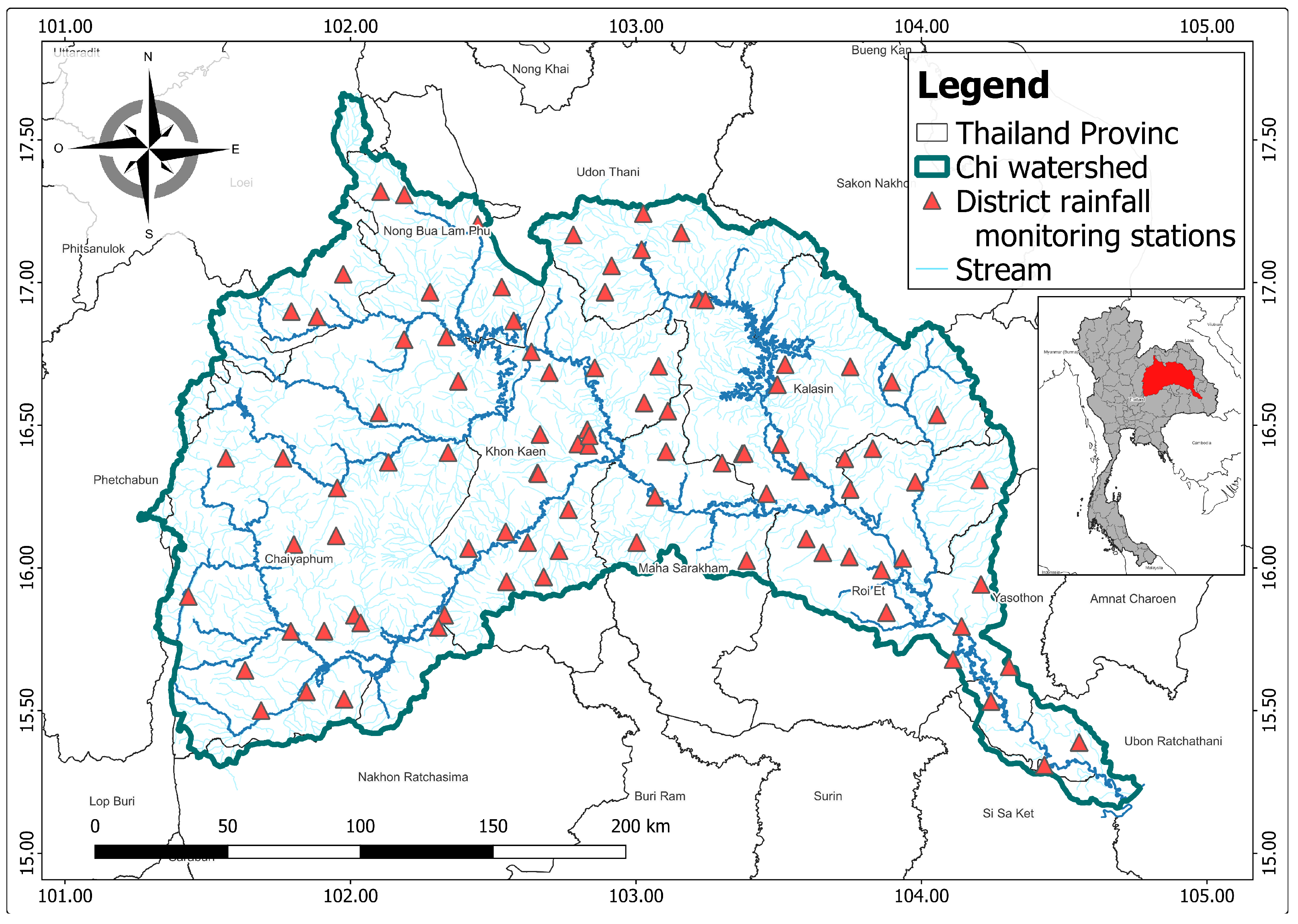
2. Study Area
3. Methodology
3.1. The GEVD
3.2. The Maximum Likelihood Estimation
3.3. The Return Level
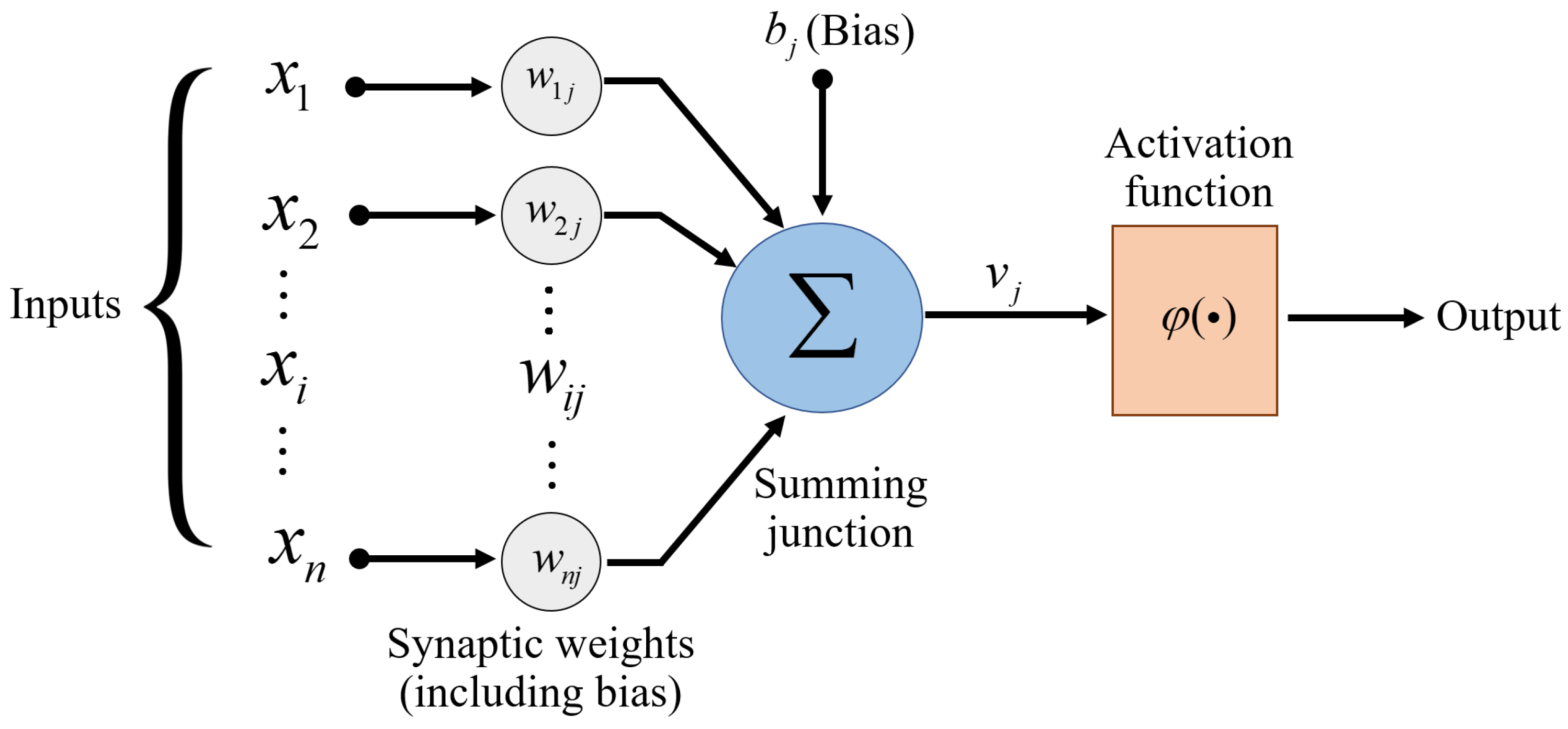
3.4. The ANN Approach
3.5. Pearson Product-Moment Correlation Coefficient
3.6. Model Accuracy Verification
3.6.1. The RMSE
3.6.2. Nash–Sutcliffe Model Efficiency Coefficient (NSE)
4. Results and Discussion
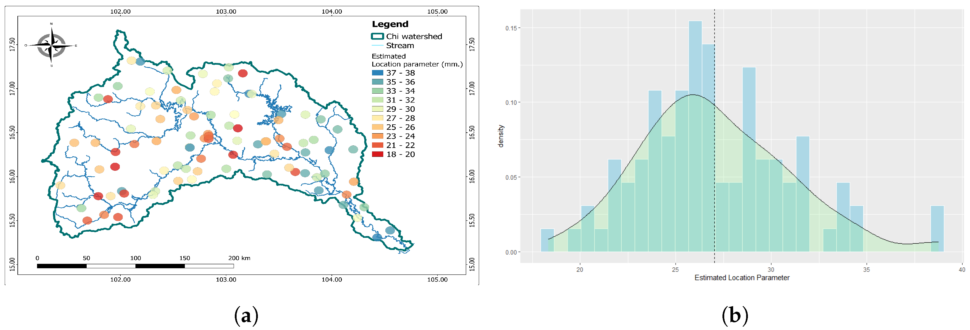
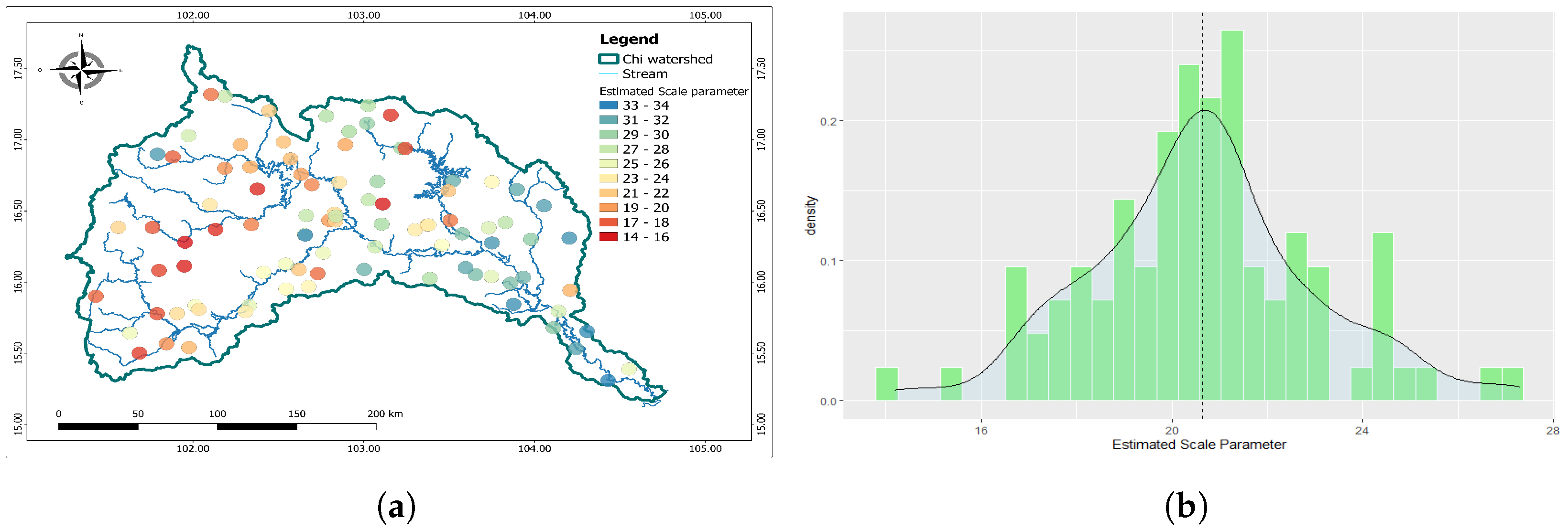
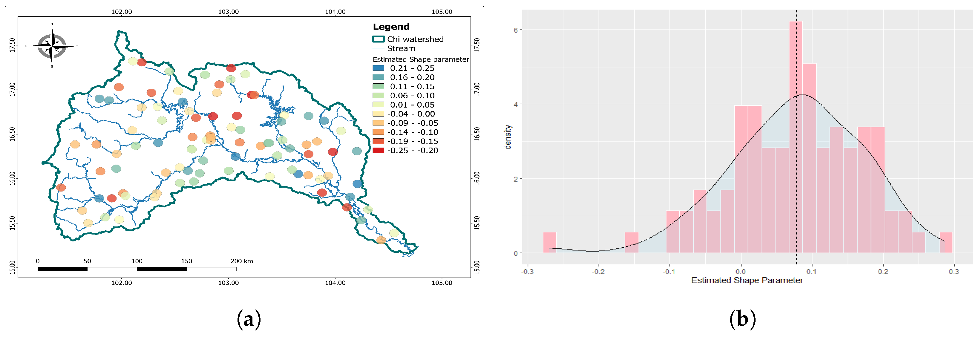
4.1. Parameter Estimation of the GEVD
4.2. Relationship between Variables
4.3. The ANN Model
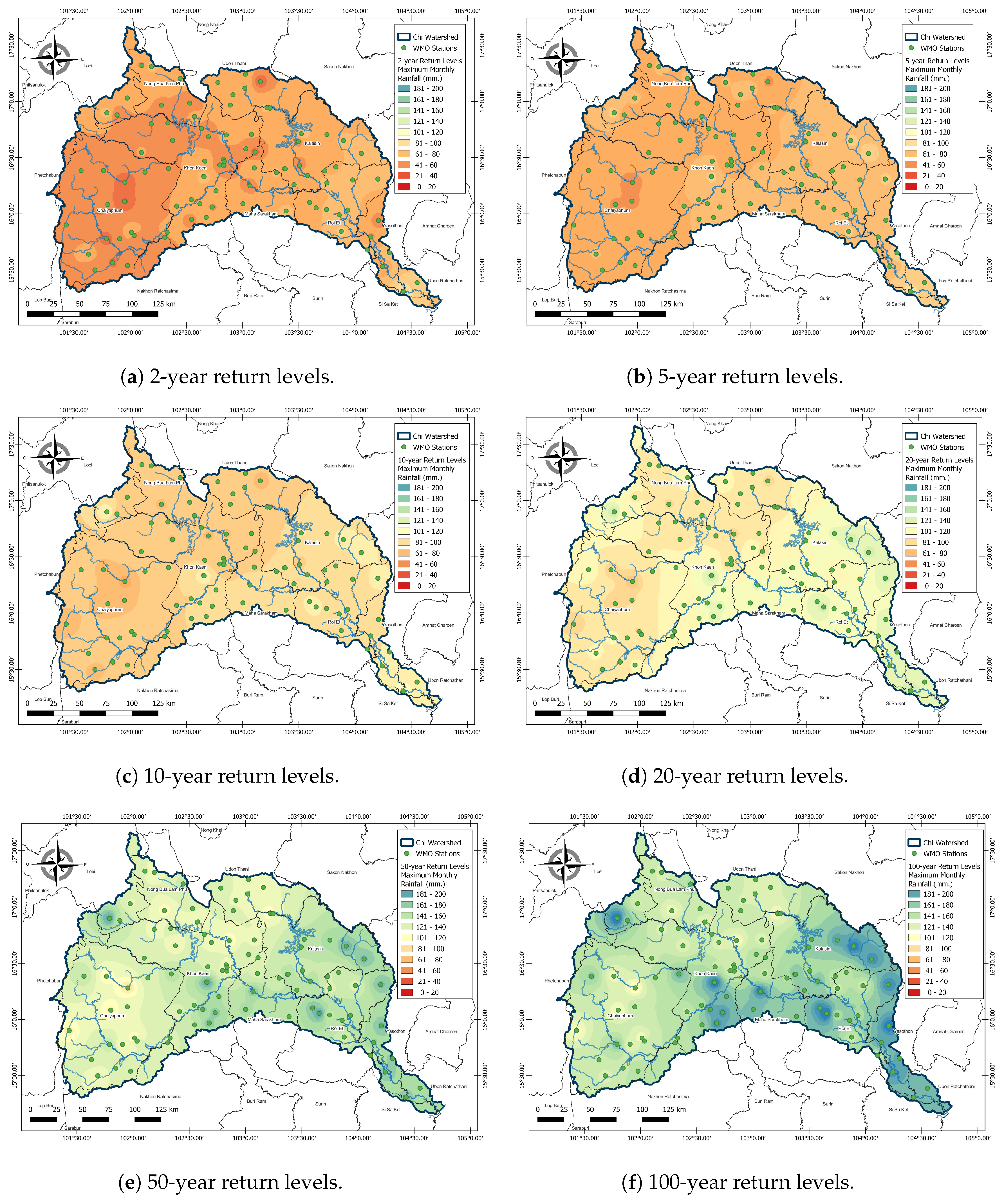
4.4. Return Level Estimation
5. Discussion
6. Conclusions
Supplementary Materials
Author Contributions
Funding
Institutional Review Board Statement
Informed Consent Statement
Data Availability Statement
Acknowledgments
Conflicts of Interest
References
- Promchote, P.; Wang, S.Y.S.; Johnson, P.G. The 2011 Great Flood in Thailand: Climate Diagnostics and Implications from Climate Change. J. Clim. 2016, 29, 367–379. [Google Scholar] [CrossRef]
- Singkran, N. Flood risk management in Thailand: Shifting from a passive to a progressive paradigm. Int. J. Dis. Risk Red. 2017, 25, 92–100. [Google Scholar] [CrossRef]
- Gale, E.L.; Saunders, M.A. The 2011 Thailand flood: Climate causes and return periods. Weather 2013, 68, 233–237. [Google Scholar] [CrossRef]
- Kunitiyawichai, K.; Schultz, B.; Uhlenbrook, S.; Suryadi, F.; Corzo, G. Comprehensive flood mitigation and management in the Chi River Basin, Thailand. Lowland Technol. Int. 2011, 13, 10–18. [Google Scholar]
- Arunyanart, N.; Limsiri, C.; Uchaipichat, A. Flood hazards in the Chi River Basin, Thailand: Impact management of climate change. Appl. Ecol. Environ. Res. 2017, 15, 841–861. [Google Scholar] [CrossRef]
- Prahadchai, T.; Shin, Y.; Busababodhin, P.; Park, J.S. Analysis of maximum precipitation in Thailand using non-stationary extreme value models. Atmos. Sci. Lett. 2022, 24, e1145. [Google Scholar] [CrossRef]
- Department, R.I. Summarizes the Situation of the Chi-Mun Watershed Flooding in 2019. 2019. Available online: http://water.rid.go.th (accessed on 15 January 2023).
- Meteorological, T. Climatic Informations. 2021. Available online: https://www.tmd.go.th (accessed on 10 January 2023).
- Shin, Y.; Shin, Y.; Hong, J.; Kim, M.K.; Byun, Y.H.; Boo, K.O.; Chung, I.U.; Park, D.S.R.; Park, J.S. Future Projections and Uncertainty Assessment of Precipitation Extremes in the Korean Peninsula from the CMIP6 Ensemble with a Statistical Framework. Atmosphere 2021, 12, 97. [Google Scholar] [CrossRef]
- Lima, C.H.; Lall, U.; Troy, T.; Devineni, N. A hierarchical Bayesian GEV model for improving local and regional flood quantile estimates. J. Hydrol. 2016, 541, 816–823. [Google Scholar] [CrossRef]
- Tyralis, H.; Papacharalampous, G.; Tantanee, S. How to explain and predict the shape parameter of the generalized extreme value distribution of streamflow extremes using a big dataset. J. Hydrol. 2019, 574, 628–645. [Google Scholar] [CrossRef]
- Jin, X.; Zhou, W.; Bie, R. Multinomial event naive Bayesian modeling for SAGE data classification. Comput. Stat. 2007, 22, 133–143. [Google Scholar] [CrossRef]
- De Luca, D.L.; Napolitano, F. A user-friendly software for modelling extreme values: EXTRASTAR (EXTRemes Abacus for STAtistical Regionalization). Environ. Model. Softw. 2023, 161, 105622. [Google Scholar] [CrossRef]
- De Michele, C. Advances in deriving the exact distribution of maximum annual daily precipitation. Water 2019, 11, 2322. [Google Scholar] [CrossRef]
- Asadi, H.; Shahedi, K.; Jarihani, B.; Sidle, R.C. Rainfall-Runoff Modelling Using Hydrological Connectivity Index and Artificial Neural Network Approach. Water 2019, 11, 212. [Google Scholar] [CrossRef]
- Lillesand, T.; Kiefer, R.; Chipman, J. Remote Sensing and Image Interpretation; John Wiley & Sons: Hoboken, NJ, USA, 2015. [Google Scholar]
- Guarnieri, R.A.; Pereira, E.; Chou, S. Solar radiation forecast using artificial neural networks in South Brazil. In Proceedings of the 8th International Conference on Southern Hemisphere Meteorology and Oceanography—8 ICSHMO, Foz do Iguaçu, Brazil, 24–28 April 2006; pp. 1777–1785. [Google Scholar]
- Ahmed, S. Performance of derivative free search ANN training algorithm with time series and classification problems. Comp. Stat. 2013, 28, 1881–1914. [Google Scholar] [CrossRef]
- Rotjanakusol, T.; Laosuwan, T. Drought Evaluation with NDVI-Based Standardized Vegetation Index in Lower Northeastern Region of Thailand. Geogr. Tech. 2019, 14, 118–130. [Google Scholar] [CrossRef]
- Land Processes Distributed Active Archive Center (LP DAAC). MOD13Q1 Version 6 Vegetation Indices. Available online: https://lpdaac.usgs.gov/products/mod13q1v006/ (accessed on 10 March 2023).
- Jenkinson, A.F. The frequency distribution of the annual maximum (or minimum) values of meteorological elements. Q. J. R. Meteorol. Soc. 1955, 81, 158–171. [Google Scholar] [CrossRef]
- Coles, S. An Introduction to Statistical Modeling of Extreme Values; Springer: New York, NY, USA, 2001. [Google Scholar]
- Busababodhin, P. Extreme Value Analysis; Rajabhat MahaSarakham University: Maha Sarakham, Thailand, 2018. [Google Scholar]
- Papukdee, N.; Park, J.S.; Busababodhin, P. Penalized likelihood approach for the four-parameter kappa distribution. J. Appl. Stat. 2022, 49, 1559–1573. [Google Scholar] [CrossRef]
- Moré, J.J. The Levenberg-Marquardt algorithm: Implementation and theory. In Numerical Analysis; Watson, G.A., Ed.; Springer: Berlin/Heidelberg, Germany, 1978; pp. 105–116. [Google Scholar]
- Kim, T.W.; Valdés, J.B. Nonlinear Model for Drought Forecasting Based on a Conjunction of Wavelet Transforms and Neural Networks. J. Hydrol. Eng. 2003, 8, 319–328. [Google Scholar] [CrossRef]
- Fritsch, S.; Guenther, F.; Guenther, M.F. Package ‘neuralnet’. Train. Neural Netw. 2019, 2, 30. [Google Scholar]
- Pearson, K. Notes on the History of Correlation. Biometrika 1920, 13, 25–45. [Google Scholar] [CrossRef]
- Nash, J.; Sutcliffe, J. River flow forecasting through conceptual models part I—A discussion of principles. J. Hydrol. 1970, 10, 282–290. [Google Scholar] [CrossRef]


| Attribute Type | Attribute | Notation |
|---|---|---|
| GEVD attributes | Location parameter | or mu |
| Scale parameter | or sigma | |
| Shape parameter | or xi | |
| Geographical coordinates | Latitude | LAT |
| Longitude | LON | |
| Meteorological variables | Maximum rainfall | max_rain |
| Average rainfall | average_rain | |
| Cumulative rainfall | sum_rain | |
| Average minimum rainfall | min_average_rain | |
| Maximum wind speed | max_wind | |
| Average wind speed | average_wind | |
| Maximum temperature | max_temp | |
| Minimum temperature | min_temp | |
| Average temperature | average_temp | |
| Average relative humidity | average_RH | |
| Maximum relative humidity | max_RH | |
| Satellite images | NDVI | NDVI |
| Hydrological variables | Maximum runoff | max_runoff |
| Average runoff | average_runoff |
| Model | Input Variable | Structure | RMSE | NSE |
|---|---|---|---|---|
| ANN01 | , , LAT, LON, max_rain, average_rain, sum_rain, min_average_rain, max_wind, average_wind, max_temp, min_temp, average_temp, average_RH, max_RH, NDVI, runoff_ max, average_runoff | 18-1-1 | 2.1848 | 0.7541 |
| ANN02 | , , LAT, LON, max_rain, average_rain, sum_rain, min_average_rain, max_wind, average_wind, max_temp, min_temp, average_temp, average_RH, max_RH, NDVI, max_runoff, Average_Runoff | 18-20-1 | 2.4424 | 0.6927 |
| ANN03 | , , LAT, LON, max_rain, average_rain, sum_rain, min_average_rain, max_wind, average_wind, max_temp | 11-4-1 | 2.3731 | 0.6837 |
| ANN04 | , LON, average_rain | 3-14-1 | 2.8328 | 0.6047 |
| ANN05 | , LON, average_rain | 3-16-1 | 2.8452 | 0.6012 |
| ANN06 | , LON, average_rain | 3-11-1 | 2.8453 | 0.6012 |
| ANN07 | max_rain, average_rain, sum_rain | 3-4-1 | 3.0436 | 0.2307 |
| ANN08 | max_rain, average_rain, sum_rain | 3-16-1 | 3.0573 | 0.2237 |
| ANN09 | max_rain, average_rain, sum_rain | 3-5-1 | 3.0665 | 0.2190 |
| Model | Input Variable | Structure | RMSE | NSE |
|---|---|---|---|---|
| ANN10 | , , LAT, LON, max_rain, average_rain, sum_rain, min_average_rain, max_wind | 9-1-1 | 1.6799 | 0.5998 |
| ANN11 | , , LAT, LON, max_rain, average_rain, sum_rain, min_average_rain, max_wind, average_wind, max_temp, min_temp, average_temp | 13-14-1 | 1.7302 | 0.5920 |
| ANN12 | , , LAT | 3-10-1 | 1.7400 | 0.5330 |
| ANN13 | 1-1-1 | 1.9115 | 0.4450 | |
| ANN14 | 1-2-1 | 1.9151 | 0.4429 | |
| ANN15 | 1-3-1 | 1.9146 | 0.4432 | |
| ANN16 | max_rain, average_rain, sum_rain, max_wind, average_wind, max_temp, min_temp, average_temp, average_RH, max_RH, NDVI, max_runoff | 12-9-1 | 1.6006 | 0.5323 |
| ANN17 | , average_rain, sum_rain, max_wind, average_wind, max_temp, min_temp, average_temp, average_RH, max_RH, NDVI, max_runoff | 12-1-1 | 1.6455 | 0.5057 |
| ANN18 | max_rain, average_rain, sum_rain, max_wind, average_wind, max_temp | 6-20-1 | 2.1025 | 0.4847 |
| Models | Input Variable | Structure | RMSE | NSE |
|---|---|---|---|---|
| ANN19 | , , LAT, LON, max_rain, average_rain, sum_rain, min_average_rain, max_wind, average_wind | 9-6-1 | 0.0740 | 0.4866 |
| ANN20 | , , LAT, LON, max_rain, average_rain | 6-2-1 | 0.0807 | 0.4669 |
| ANN21 | , , LAT, LON, max_rain, average_rain | 6-16-1 | 0.0833 | 0.4319 |
| ANN22 | , LAT, LON, average_rain, sum_rain | 5-17-1 | 0.0651 | 0.4734 |
| ANN23 | , LAT, LON, average_rain, sum_rain | 5-2-1 | 0.0673 | 0.4374 |
| ANN24 | , LAT, LON, average_rain, sum_rain, average_wind, max_temp, min_temp, average_temp, average_RH, NDVI, min_average_rain | 12-4-1 | 0.0843 | 0.4250 |
| ANN25 | max_rain, average_rain, sum_rain, max_wind | 4-19-1 | 0.0803 | 0.0931 |
| ANN26 | max_rain, average_rain, sum_rain, max_wind | 4-16-1 | 0.0804 | 0.0903 |
| ANN27 | max_rain, average_rain, sum_rain, max_wind | 4-10-1 | 0.0807 | 0.0826 |
| Model | Parameters Estimations Process | Number of Stations (Percentage) | ||
|---|---|---|---|---|
| (mu) | (sigma) | (xi) | ||
| GEVD01 | S | S | S | 10 (10.87%) |
| GEVD02 | S | NS | S | 15 (16.30%) |
| GEVD03 | S | NS | NS | 11 (11.96%) |
| GEVD04 | S | S | NS | 7 (7.61%) |
| GEVD05 | NS | NS | NS | 7 (7.61%) |
| GEVD06 | NS | NS | S | 11 (11.96%) |
| GEVD07 | NS | S | S | 15 (16.30%) |
| GEVD08 | NS | S | NS | 16 (17.39%) |
Disclaimer/Publisher’s Note: The statements, opinions and data contained in all publications are solely those of the individual author(s) and contributor(s) and not of MDPI and/or the editor(s). MDPI and/or the editor(s) disclaim responsibility for any injury to people or property resulting from any ideas, methods, instructions or products referred to in the content. |
© 2023 by the authors. Licensee MDPI, Basel, Switzerland. This article is an open access article distributed under the terms and conditions of the Creative Commons Attribution (CC BY) license (https://creativecommons.org/licenses/by/4.0/).
Share and Cite
Phoophiwfa, T.; Laosuwan, T.; Volodin, A.; Papukdee, N.; Suraphee, S.; Busababodhin, P. Adaptive Parameter Estimation of the Generalized Extreme Value Distribution Using Artificial Neural Network Approach. Atmosphere 2023, 14, 1197. https://doi.org/10.3390/atmos14081197
Phoophiwfa T, Laosuwan T, Volodin A, Papukdee N, Suraphee S, Busababodhin P. Adaptive Parameter Estimation of the Generalized Extreme Value Distribution Using Artificial Neural Network Approach. Atmosphere. 2023; 14(8):1197. https://doi.org/10.3390/atmos14081197
Chicago/Turabian StylePhoophiwfa, Tossapol, Teerawong Laosuwan, Andrei Volodin, Nipada Papukdee, Sujitta Suraphee, and Piyapatr Busababodhin. 2023. "Adaptive Parameter Estimation of the Generalized Extreme Value Distribution Using Artificial Neural Network Approach" Atmosphere 14, no. 8: 1197. https://doi.org/10.3390/atmos14081197
APA StylePhoophiwfa, T., Laosuwan, T., Volodin, A., Papukdee, N., Suraphee, S., & Busababodhin, P. (2023). Adaptive Parameter Estimation of the Generalized Extreme Value Distribution Using Artificial Neural Network Approach. Atmosphere, 14(8), 1197. https://doi.org/10.3390/atmos14081197