


Long Memory Cointegration in the Analysis of Maximum, Minimum and Range Temperatures in Africa: Implications for Climate Change
 , , and
Abstract
1. Introduction
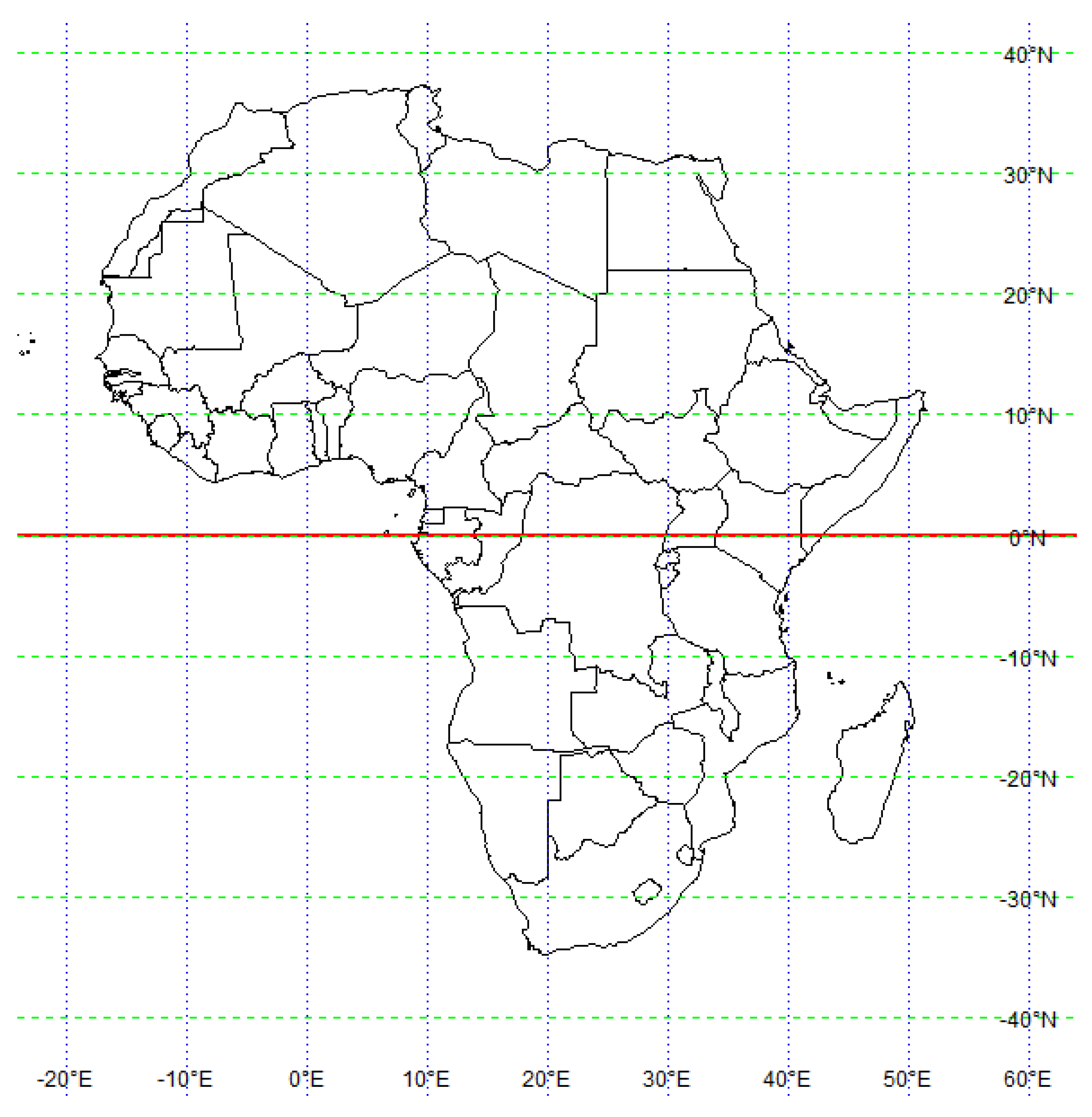
2. Data
3. Econometric Methods
3.1. Testing for a Linear Trend
3.2. Testing for Fractional Integration
3.3. Homogeneity of Paired Fractional Integration Parameters
3.4. Narrow-Band Frequency Domain Least Square Approach
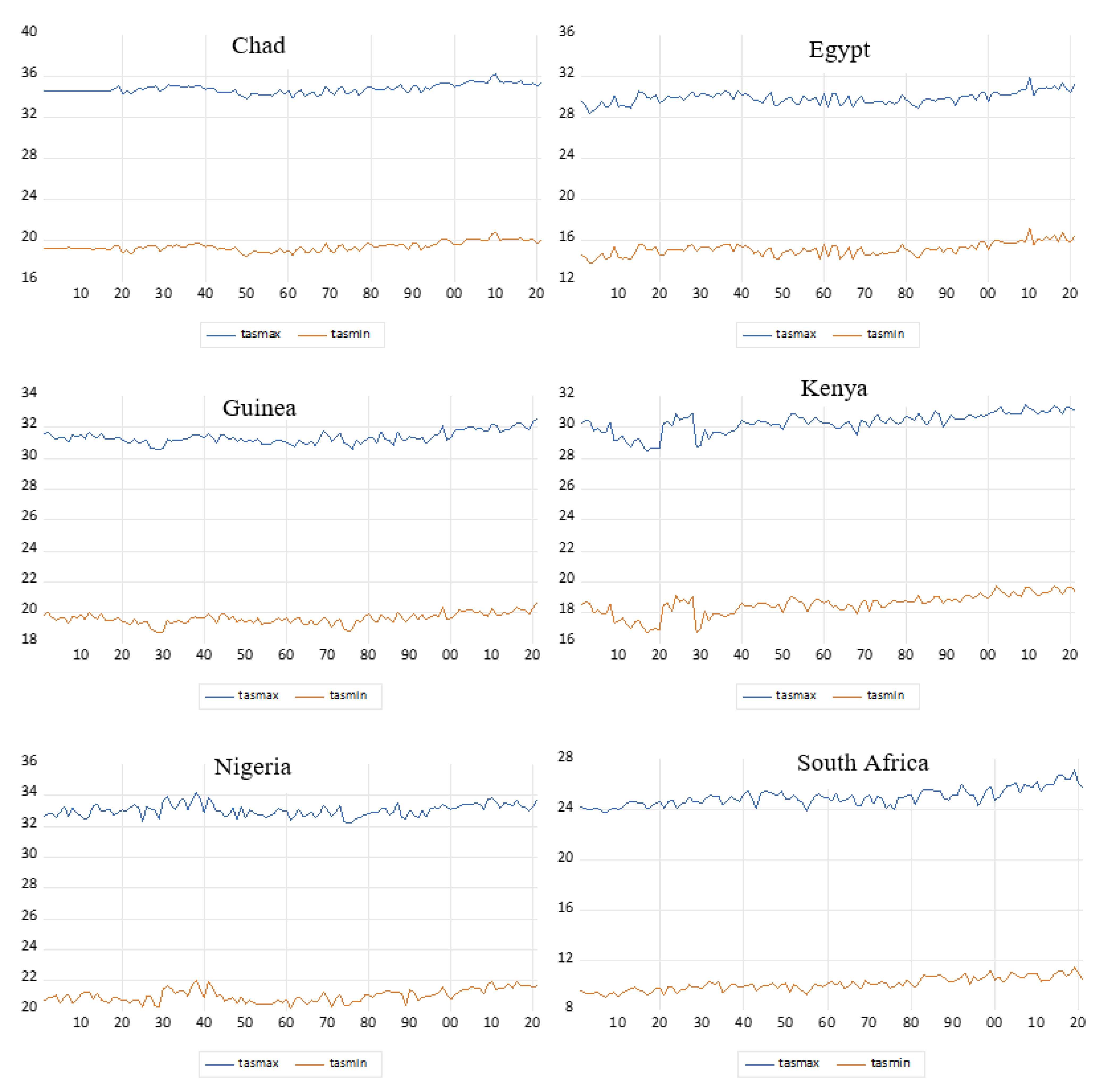
4. Main Results
5. Conclusions
Author Contributions
Funding
Institutional Review Board Statement
Informed Consent Statement
Data Availability Statement
Acknowledgments
Conflicts of Interest
References
- FAO. Climate Change and Food Security in Africa: A Review of the Status, Challenges and Opportunities; FAO: Rome, Italy, 2021. [Google Scholar]
- IPCC Global Warming of 1.5 °C—An IPCC Special Report on the Impacts of Global Warming of 1.5 °C above Pre-Industrial Levels and Related Global Greenhouse Gas Emission Pathways, in the Context of Strengthening the Global Response to the Threat of Climate Change, Sustainable Development, and Efforts to Eradicate Poverty. 2018. Available online: https://www.ipcc.ch/sr15/ (accessed on 18 July 2023).
- Nicholls, N.; Gruza, G.V.; Jouzel, J.; Karl, T.R.; Ogallo, L.A.; Parker, D.E. Observed climate variability and change. In Climate Change 1995: The Science of Climate Change; Houghton, J.T., Meiro Filho, L.G., Callendar, B.A., Kattenburg, A., Maskell, K., Eds.; Cambridge University Press: Cambridge, UK, 1996; pp. 133–192. [Google Scholar]
- Percival, D.B.; Overland, J.E.; Mofjeld, H.O. Interpretation of North Pacific Variability as a Short- and Long-Memory Process*. J. Clim. 2001, 14, 4545–4559. [Google Scholar] [CrossRef]
- Caballero, R.; Jewson, S.; Brix, A. Long memory in surface air temperature: Detection, modeling, and application to weather derivative valuation. Clim. Res. 2002, 21, 127–140. [Google Scholar] [CrossRef]
- Gil-Alana, L.A. Time trends with breaks and fractional integration in temperature time series. Clim. Chang. 2008, 9, 325–337. [Google Scholar] [CrossRef]
- Franzke, C. Nonlinear Trends, Long-Range Dependence, and Climate Noise Properties of Surface Temperature. J. Clim. 2012, 25, 4172–4183. [Google Scholar] [CrossRef]
- Ludescher, J.; Bunde AFranzke, C.L.; Schellnhuber, H.J. Long-term persistence enhances uncertainty about anthropo-genic warming of Antarctica. Clim. Dyn. 2016, 46, 263–271. [Google Scholar] [CrossRef]
- Contractor, S.; Donat, M.G.; Alexander, L.V. Changes in Observed Daily Precipitation over Global Land Areas since 1950. J. Clim. 2020, 34, 3–19. [Google Scholar] [CrossRef]
- Karl, T.R.; Kukla, G.; Razuvayev, V.N.; Changery, M.J.; Quayle, R.G.; Heim, R.R., Jr.; Easterling, D.R.; Fu, C.B. Global Warming: Evidence for asymmetric diurnal temperature change. Geophys. Res. Lett. 1991, 18, 2253–2256. [Google Scholar] [CrossRef]
- Hansen, J.E.; Ruedy, R.; Sato, M.; Lo, K. Global surface temperature change. Rev. Geophys. 2010, 48, RG4004. [Google Scholar] [CrossRef]
- Cahill, N.; Rahmstorf, S.; Parnell, A.C. Change points of global temperature. Environ. Res. Lett. 2015, 10, 084002. [Google Scholar] [CrossRef]
- Shepard, D. Global Warming: Severe Consequences for Africa. United Nations African Renewal. 2019. Available online: https://www.un.org/africarenewal/magazine/december-2018-march-2019/global-warming-severe-consequences-africa (accessed on 16 May 2022).
- Ray, C.A. The Impact of Climate Change on Africa’s Economies. African Program, Analysis, Foreign Policy Research Institute, Pennsylvania, USA. 2021. Available online: https://www.fpri.org/article/2021/10/the-impact-of-climate-change-on-africas-economies/ (accessed on 16 May 2022).
- IPCC AR6 Climate Change 2021: The Physical Science Basis. IPCC Sixth Assessment Report Working Group 1. 2021. Available online: https://www.ipcc.ch/report/sixth-assessment-report-working-group-i/ (accessed on 15 July 2023).
- Ngarukiyimana, J.B.; Ruhinda, B.; Mupenzi, J. Climate change and adaptation strategies for agricultural sector in Rwan-da: A review. Environ. Dev. Sustain. 2020, 22, 209–233. [Google Scholar]
- CDKN. The IPCC’s Fifth Assessment Report What’s in it for Africa? 2014. Available online: http://cdkn.org/wp-content/uploads/2014/04/AR5_IPCC_Whats_in_it_for_Africa.pdf (accessed on 20 June 2016).
- Kruger, A.C.; Sekele, S.S. Trends in extreme temperature indices in South Africa: 1962–2009. Int. J. Clim. 2012, 33, 661–676. [Google Scholar] [CrossRef]
- Kruger, A.C.; Nxumalo, M. Surface temperature trends from homogenized time series in South Africa: 1931–2015. Int. J. Clim. 2016, 37, 2364–2377. [Google Scholar] [CrossRef]
- New, M.; Hewitson, B.; Stephenson, D.B.; Tsiga, A.; Kruger, A.; Manhique, A.; Gomez, B.; Coelho, C.A.S.; Masisi, D.N.; Kululanga, E.; et al. Evidence of trends in daily climate extremes over southern and west Africa. J. Geophys. Res. Atmos. 2006, 111, D14102. [Google Scholar] [CrossRef]
- Neumann, R.; Jung, G.; Laux, P.; Kunstmann, H. Climate trends of temperature, precipitation and river discharge in the Volta Basin of West Africa. Int. J. River Basin Manag. 2007, 5, 17–30. [Google Scholar] [CrossRef]
- Muthoni, F. Spatial-Temporal Trends of Rainfall, Maximum and Minimum Temperatures Over West Africa. IEEE J. Sel. Top. Appl. Earth Obs. Remote Sens. 2020, 13, 2960–2973. [Google Scholar] [CrossRef]
- Gil-Alana, L.A.; Yaya, O.S.; Fagbamigbe, A.F. Time series analysis of quarterly rainfall and temperature (1900–2012) in sub-Saharan African countries. Theor. Appl. Clim. 2019, 137, 61–76. [Google Scholar] [CrossRef]
- Yaya, O.S.; Fashae, O.A. Seasonal fractional integrated time series models for rainfall data in Nigeria. Theor. Appl. Clim. 2015, 120, 99–108. [Google Scholar] [CrossRef]
- Yaya, O.S.; Gil-Alana, L.A.; Akomolafe, A.A. Long Memory, Seasonality and Time Trends in the Average Monthly Rainfall in Major cities of Nigeria. CBN J. Appl. Stat. 2015, 6, 39–58. [Google Scholar]
- Ogunsola, O.; Yaya, O. Maximum and Minimum Temperatures in South-Western Nigeria: Time trends, Seasonality and Persistence. J. Phys. Conf. Ser. 2019, 1299, 012057. [Google Scholar] [CrossRef]
- Yaya, O.S.; Akintande, O.J. Long range dependence, Nonlinear trend and Breaks in historical Sea-surface and Land-air-surface Global and Regional Temperature anomalies. Theor. Appl. Climatol. 2019, 137, 177–185. [Google Scholar] [CrossRef]
- Yaya, O.S.; Vo, X.V. Statistical Analysis of Rainfall and Temperature (1901–2016) in South-East Asian Region. Theor. Appl. Climatol. 2020, 142, 287–303. [Google Scholar] [CrossRef]
- Carcel, H.; Gil-Alana, L.A. Climate Warming: Is There Evidence in Africa? Adv. Meteorol. 2015, 2015, 917603. [Google Scholar] [CrossRef][Green Version]
- Robinson, P.M.; Yajima, Y. Determination of cointegrating rank in fractional systems. J. Econ. 2002, 106, 217–241. [Google Scholar] [CrossRef]
- Christensen, B.J.; Nielsen, M.Ø. Asymptotic normality of narrow-band least squares in the stationary fractional cointe-gration model and volatility forecasting. J. Econom. 2006, 133, 343–371. [Google Scholar] [CrossRef]
- Marinucci, D.; Robinson, P. Semiparametric fractional cointegration analysis. J. Econ. 2001, 105, 225–247. [Google Scholar] [CrossRef]
- Hamilton, J.D. Time Series Analysis; Princeton University Press: Princeton, NJ, USA, 1994; 820p. [Google Scholar]
- Montanari, A.; Rosso, R.; Taqqu, M.S. Some long-run properties of rainfall records in Italy. J. Geophys. Res. Atmos. 1996, 101, 29431–29438. [Google Scholar] [CrossRef]
- Stephenson, D.B.; Pavan, V.; Bojariu, R. Is the North Atlantic oscillation a random walk? Int. J. Climatol. 2000, 20, 1–18. [Google Scholar] [CrossRef]
- Gil-Alana, L.A. An application of fractional integration to a long temperature time series. Int. J. Climatol. 2003, 23, 1699–1710. [Google Scholar] [CrossRef]
- Gil-Alana, L.A. Statistical Modeling of the Temperatures in the Northern Hemisphere Using Fractional Integration Techniques. J. Clim. 2005, 18, 5357–5369. [Google Scholar] [CrossRef]
- Gil-Alana, L.A. Long memory, seasonality and time trends in the average monthly temperatures in Alaska. Theor. Appl. Clim. 2012, 108, 385–396. [Google Scholar] [CrossRef]
- Dahlhaus, R. Efficient Parameter Estimation for Self-Similar Processes. Ann. Stat. 1989, 17, 1749–1766. [Google Scholar] [CrossRef]
- Robinson, P.M. Efficient Tests of Nonstationary Hypotheses. J. Am. Stat. Assoc. 1994, 89, 1420–1437. [Google Scholar] [CrossRef]
- Robinson, P.M. Semiparametric Analysis of Long-Memory Time Series. Ann. Stat. 1994, 22, 515–539. [Google Scholar] [CrossRef]
- Robinson, P.M. Gaussian Semiparametric Estimation of Long Range Dependence. Ann. Stat. 1995, 23, 1630–1661. [Google Scholar] [CrossRef]
- Yaya, O.S. Compendium of Time Series Econometrics with Applications; Ibadan University Printery: Ibadan, Nigeria, 2022. [Google Scholar]
- Robinson, P.M.; Hidalgo, F.J. Time series regression with long-range dependence. Ann. Stat. 1997, 25, 77–104. [Google Scholar] [CrossRef]
- Dickey, D.A.; Fuller, W.A. Distribution of the estimators for autoregressive time series with a unit root. J. Am. Stat. Assoc. 1979, 74, 427–431. [Google Scholar]
- Diebold Francis, X.; Rudebusch Glenn, D. On the power of Dickey-Fuller tests against fractional alternatives. Econ. Lett. 1991, 35, 155–160. [Google Scholar] [CrossRef]
- Hassler, U.; Wolters, J. On the power of unit root tests against fractional alternatives. Econ. Lett. 1994, 45, 1–5. [Google Scholar] [CrossRef]
- Lee, D.; Schmidt, P. On the power of the KPSS test of stationarity against fractionally-integrated alternatives. J. Econ. 1996, 73, 285–302. [Google Scholar] [CrossRef]
- Engle, R.; Granger, C.W.J. Cointegration and error correction. Representation, estimation and testing. Econometrica 1987, 55, 251–276. [Google Scholar] [CrossRef]
- Nielsen, M.O. Multivariate Fractional Integration and Cointegration. Ph.D. Thesis, University of Aarhus, Aarhus, Denmark, 2015. [Google Scholar]
- Guo, Y.; Wang, X. Climate change and its impact of China’s agricultural production. Int. J. Glob. Warm. 2015, 7, 437–450. [Google Scholar]
- Diebold, F.X.; Inoue, A. Long memory and regime switching. J. Econ. 2001, 105, 131–159. [Google Scholar] [CrossRef]
- Granger, C.W.; Hyung, N. Occasional structural breaks and long memory with an application to the S&P 500 absolute stock returns. J. Empir. Financ. 2004, 11, 399–421. [Google Scholar] [CrossRef]
- Cuestas, J.; Gil-Alana, L.A. A nonlinear approach with long range dependence based on Chebyshev polynomials. Stud. Nonlinear Dyn. Econom. 2016, 16, 445–468. [Google Scholar]
- Gil-Alana, L.A.; Yaya, O.S. Testing fractional unit roots with non-linear smooth break approximations using Fourier functions. J. Appl. Stat. 2021, 48, 2542–2559. [Google Scholar] [CrossRef] [PubMed]
- Yaya, O.S.; Ogbonna, A.E.; Furuoka, R.; Gil-Alana, L.A. A new unit root test for unemployment hysteresis based on the autoregressive neural network. Oxford Bull. Econ. Statistics 2021, 83, 960–981. [Google Scholar] [CrossRef]


| Country | Max. Temp (°C) | Min. Temp (°C) | Range (°C) | |||
|---|---|---|---|---|---|---|
| 1901 | 2021 | 1901 | 2021 | 1901 | 2021 | |
| Angola | 28.18 | 28.60 | 14.51 | 14.93 | 13.67 | 13.67 |
| Benin | 33.23 | 34.47 | 21.58 | 22.98 | 11.65 | 11.49 |
| Botswana | 29.08 | 29.81 | 13.16 | 13.72 | 15.92 | 16.09 |
| Burkina Faso | 34.46 | 36.27 | 21.78 | 23.81 | 12.68 | 12.46 |
| Cameroon | 29.51 | 30.59 | 18.84 | 19.87 | 10.67 | 10.72 |
| Central Afr. Rep. | 31.34 | 32.16 | 18.60 | 19.45 | 12.74 | 12.71 |
| Chad | 34.58 | 35.42 | 19.32 | 20.06 | 15.26 | 15.36 |
| Congo | 28.77 | 29.77 | 19.72 | 20.73 | 9.05 | 9.04 |
| Cote d’Ivoire | 31.67 | 32.54 | 21.42 | 22.26 | 10.25 | 10.28 |
| Egypt | 29.64 | 31.27 | 14.69 | 16.53 | 14.95 | 14.74 |
| Gabon | 28.69 | 29.84 | 20.36 | 21.51 | 8.33 | 8.33 |
| Ghana | 32.17 | 33.4 | 21.97 | 23.25 | 10.2 | 10.15 |
| Guinea | 31.57 | 32.53 | 19.86 | 20.69 | 11.71 | 11.84 |
| Guinea-Bissau | 33.74 | 34.99 | 21.4 | 22.59 | 12.34 | 12.40 |
| Kenya | 30.28 | 31.11 | 18.51 | 19.39 | 11.77 | 11.72 |
| Lesotho | 17.24 | 19.45 | 4.35 | 5.11 | 12.89 | 14.34 |
| Liberia | 30.38 | 30.50 | 21.17 | 21.30 | 9.21 | 9.20 |
| Libya | 28.77 | 29.87 | 15.21 | 16.28 | 13.56 | 13.59 |
| Madagascar | 27.39 | 27.63 | 17.92 | 18.16 | 9.47 | 9.47 |
| Malawi | 27.23 | 28.10 | 16.41 | 17.54 | 10.82 | 10.56 |
| Mali | 35.28 | 36.93 | 20.99 | 22.68 | 14.29 | 14.25 |
| Mauritania | 34.65 | 36.02 | 21.27 | 22.62 | 13.38 | 13.40 |
| Morocco | 23.26 | 24.52 | 11.39 | 12.49 | 11.87 | 12.03 |
| Namibia | 27.34 | 27.62 | 12.28 | 12.66 | 15.06 | 14.96 |
| Niger | 34.77 | 35.70 | 19.99 | 20.52 | 14.78 | 15.18 |
| Nigeria | 32.63 | 33.74 | 20.69 | 21.65 | 11.94 | 12.09 |
| Rwanda | 24.88 | 25.29 | 12.78 | 13.19 | 12.10 | 12.10 |
| Sierra Leone | 31.69 | 32.25 | 21.70 | 22.18 | 9.99 | 10.07 |
| Senegal | 35.51 | 36.91 | 21.09 | 22.39 | 14.42 | 14.52 |
| South Africa | 24.25 | 25.73 | 9.55 | 10.44 | 14.70 | 15.29 |
| Sudan | 35.61 | 35.89 | 19.92 | 20.51 | 15.69 | 15.38 |
| Tanzania | 27.90 | 28.50 | 16.53 | 17.55 | 11.37 | 10.95 |
| Tunisia | 25.20 | 27.07 | 12.97 | 15.65 | 12.23 | 11.42 |
| Uganda | 28.67 | 29.34 | 16.55 | 17.14 | 12.12 | 12.20 |
| Zambia | 28.50 | 29.06 | 14.60 | 15.22 | 13.90 | 13.84 |
| Zimbabwe | 27.80 | 28.64 | 14.25 | 15.14 | 13.55 | 13.50 |
| Country | Max. Temp (°C) | Min. Temp (°C) | Range (°C) | ||||||
|---|---|---|---|---|---|---|---|---|---|
| None | Intercept | Intercept + Trend | None | Intercept | Intercept + Trend | None | Intercept | Intercept + Trend | |
| Angola | 0.3171[2] | −3.1469[1] | −4.5576[1] | 0.3355[2] | −3.1752[1] | −5.5564[0] | 0.0020[4] | −5.6877[1] | −5.7386[1] |
| Benin | 0.3490[2] | −3.9137[1] | −3.9400[1] | 0.4778[3] | −2.6479[1] | −5.0183[0] | −0.1613[1] | −3.3023[1] | −5.7028[0] |
| Botswana | 0.3105[2] | −2.5926[2] | −7.6741[0] | 0.2941[2] | −4.6700[0] | −7.1066[0] | 0.1823[4] | −8.9667[0] | −9.3857[0] |
| Burkina Faso | 0.3541[1] | −5.7067[0] | −6.3192[0] | 0.5060[3] | −3.4801[0] | −5.3749[0] | −0.2151[2] | −2.8794[1] | −4.1499[1] |
| Cameroon | 0.5978[3] | −6.8662[0] | −7.5844[0] | 0.6235[2] | −2.2884[2] | −2.7278[2] | −0.1049[3] | −8.0343[0] | −8.0094[0] |
| Central Afr. Rep. | 0.5203[2] | −2.4402[2] | −3.2942[2] | 0.5388[2] | −2.1126[2] | −3.0607[2] | −0.4083[4] | −2.7591[2] | −3.2665[2] |
| Chad | 0.4917[2] | −1.5969[2] | −2.1705[2] | 0.4425[2] | −1.5745[2] | −2.4938[2] | 0.0663[2] | −3.2194[2] | −6.7898[0] |
| Congo | 0.7671[2] | −1.5726[2] | −2.5181[2] | 0.7625[2] | −1.5746[2] | −2.5178[2] | −0.3702[7] | −10.4267[0] | −10.3999[0] |
| Cote d’Ivoire | 0.6385[3] | −2.2845[2] | −2.9577[2] | 0.4687[3] | −4.2075[0] | −5.5144[0] | 0.0725[1] | −3.8767[1] | −4.3940[1] |
| Egypt | 1.3401[5] | −2.4317[2] | −2.8386[2] | 0.8076[2] | −2.2244[2] | −2.9386[2] | −0.1216[3] | −2.2496[3] | −7.6871[0] |
| Gabon | 0.8330[2] | −1.4901[2] | −2.3948[2] | 0.8256[2] | −1.4763[2] | −2.3920[2] | 0.1416[3] | −10.1007[0] | −10.1330[0] |
| Ghana | 0.5132[2] | −3.4754[1] | −3.7306[1] | 0.4655[3] | −3.8136[0] | −5.1423[0] | −0.0556[2] | −3.4082[1] | −4.4562[1] |
| Guinea | 0.6804[3] | −1.4924[2] | −2.5401[2] | 0.3832[2] | −1.9008[2] | −5.5536[0] | 0.1458[1] | −3.4493[1] | −3.6109[1] |
| Guinea-Bissau | 0.7792[3] | −0.6981[3] | −1.9087[3] | 0.6523[3] | −1.6596[2] | −2.8914[2] | 0.0566[1] | −5.5719[0] | −5.7066[0] |
| Kenya | 0.2804[2] | −1.7647[2] | −5.8075[0] | 0.3017[2] | −1.6298[2] | −6.2287[0] | −0.1759[2] | −9.8508[0] | −10.3136[0] |
| Lesotho | 1.2995[4] | −1.9224[2] | −6.8761[0] | 0.6396[3] | −1.7927[3] | −8.3858[0] | 0.9444[4] | −3.4123[1] | −3.8653[1] |
| Liberia | 0.1592[2] | −2.4895[2] | −2.88994[2] | 0.1373[2] | −2.5105[2] | −2.9140[2] | 0.0055[1] | −3.4392[1] | −3.43039[1] |
| Libya | 0.8349[3] | −1.6497[2] | −2.8180[2] | 1.0739[4] | −1.5606[2] | −2.7181[2] | 0.0138[3] | −3.2888[2] | −3.2934[2] |
| Madagascar | 0.0635[2] | −2.1187[2] | −1.9551[2] | 0.0487[2] | −2.1117[2] | −1.9450[2] | 0.3742[4] | −11.5073[0] | −11.5446[0] |
| Malawi | 0.2509[2] | −2.7236[2] | −7.6837[0] | 0.8124[5] | −5.4000[0] | −6.7249[0] | −0.2075[3] | −8.4672[0] | −8.4866[0] |
| Mali | 0.3529[1] | −3.5324[1] | −6.9707[0] | 0.3714[1] | −2.7152[1] | −5.9485[0] | −0.0972[2] | −3.1696[1] | −3.6366[1] |
| Mauritania | 0.5921[3] | −1.5369[3] | −8.0244[0] | 0.5942[3] | −1.3504[3] | −6.4320[0] | −0.0422[1] | −5.4342[0] | −5.4130[0] |
| Morocco | 0.7185[2] | −1.3661[2] | −2.9879[2] | 0.4502[2] | −2.8884[1] | −4.5408[1] | 0.1326[1] | −5.8760[0] | −7.1333[0] |
| Namibia | 0.2682[2] | −4.3714[0] | −5.8074[0] | 0.4270[3] | −3.8688[0] | −5.4211[0] | −0.1240[1] | −5.3411[1] | −5.4117[1] |
| Niger | 0.2721[2] | −2.5021[2] | −2.6363[2] | 0.2250[3] | −1.9597[3] | −3.1829[2] | 0.0795[2] | −3.0056[2] | −3.1562[2] |
| Nigeria | 0.4313[3] | −3.0302[2] | −3.1060[2] | 0.4166[2] | −2.1146[2] | −2.6235[2] | −0.3924[5] | −5.3338[1] | −8.1575[0] |
| Rwanda | 0.1542[2] | −1.5675[2] | −5.2979[0] | 0.1774[2] | −1.9275[2] | −6.3444[0] | −0.1543[2] | −3.4441[1] | −3.5358[1] |
| Sierra Leone | 0.3976[2] | −1.5657[2] | −2.3501[2] | 0.3002[2] | −1.9091[2] | −2.6355[2] | 0.2008[2] | −3.2376[1] | −3.3123[1] |
| Senegal | 0.7078[3] | −1.0306[3] | −6.1205[0] | 0.4334[2] | −2.0313[2] | −6.1411[0] | 0.0830[1] | −5.3179[0] | −5.5103[0] |
| South Africa | 0.9217[3] | −2.1540[2] | −6.4079[0] | 0.9368[3] | −1.5133[3] | −8.3558[0] | 0.5516[4] | −4.0968[1] | −4.2192[1] |
| Sudan | 0.2813[2] | −2.0396[2] | −2.3404[2] | 0.5028[2] | −1.2508[2] | −2.3882[2] | −0.5557[3] | −0.9761[3] | −6.9848[0] |
| Tanzania | 0.2266[2] | −1.7813[2] | −6.7236[0] | 0.4748[2] | −1.4784[2] | −6.4684[0] | −0.2570[1] | −4.5037[1] | −4.4851[1] |
| Tunisia | 1.1141[3] | −0.6051[3] | −4.5628[1] | 1.0992[3] | −0.9542[3] | −3.9033[1] | −0.3608[1] | −6.2147[0] | −6.3774[0] |
| Uganda | 0.2406[2] | −1.6153[2] | −5.3460[0] | 0.2176[2] | −1.5610[2] | −6.0091[0] | −0.0973[2] | −8.7951[0] | −8.8230[0] |
| Zambia | 0.1086[2] | −3.6010[1] | −4.7715[1] | 0.2810[4] | −5.5308[0] | −6.4403[0] | −0.0471[3] | −4.3075[1] | −4.5314[1] |
| Zimbabwe | 0.1805[2] | −2.5659[2] | −8.0439[0] | 0.6485[5] | −5.6556[0] | −7.2592[0] | −0.0185[4] | −9.1363[0] | −9.4686[0] |
| Country | Max. Temp (°C) | Min. Temp (°C) | Range (°C) | ||||||
|---|---|---|---|---|---|---|---|---|---|
| Intercept | Trend | Intercept | Trend | Intercept | Trend | ||||
| Angola | 0.31 (0.17, 0.45) | −0.2675 (−2.68) | 0.0045 (3.45) | 0.37 (0.22, 0.52) | −0.2532 (−2.39) | 0.0043 (3.10) | 0.11 (−0.03, 0.26) | −0.0131 (−0.61) | 0.0002 (0.75) |
| Benin | 0.43 (0.29, 0.58) | −0.1435 (−0.47) | 0.0034 (0.84) | 0.52 (0.37, 0.67) | −0.4087 (−1.11) | 0.0094 (1.97) | 0.49 (0.32, 0.66) | 0.2755 (0.97) | −0.0057 (−1.54) |
| Botswana | 0.26 (0.11, 0.41) | −0.6811 (−3.61) | 0.0115 (4.61) | 0.30 (0.15, 0.45) | −0.5774 (−3.66) | 0.0096 (4.64) | 0.13 (−0.02, 0.28) | −0.1067 (−1.57) | 0.0018 (1.90) |
| Burkina Faso | 0.41 (0.25, 0.57) | −0.2738 (−0.88) | 0.0059 (1.47) | 0.50 (0.34, 0.67) | −0.5762 (−1.41) | 0.0125 (2.40) | 0.49 (0.34, 0.64) | 0.3700 (1.37) | −0.0066 (−1.88) |
| Cameroon | 0.26 (0.11, 0.42) | −0.1617 (−1.48) | 0.0030 (2.11) | 0.35 (0.23, 0.48) | −0.1904 (−1.36) | 0.0039 (2.16) | 0.24 (0.09, 0.39) | 0.0350 (0.34) | −0.0007 (−0.52) |
| Central Afr. Rep. | 0.40 (0.25, 0.55) | −0.2546 (−1.64) | 0.0047 (2.34) | 0.41 (0.27, 0.55) | −0.2927 (−1.76) | 0.0056 (2.57) | 0.25 (0.13, 0.37) | 0.0459 (1.54) | −0.0008 (−2.14) |
| Chad | 0.47 (0.34, 0.59) | −0.3542 (−1.43) | 0.0069 (2.14) | 0.47 (0.34, 0.60) | −0.3864 (−1.61) | 0.0075 (2.42) | 0.36 (0.22, 0.51) | 0.0398 (0.61) | −0.0007 (−0.88) |
| Congo | 0.38 (0.24, 0.52) | −0.2349 (−1.71) | 0.0047 (2.64) | 0.38 (0.24, 0.53) | −0.2347 (−1.69) | 0.0047 (2.62) | 0.03 (−0.14, 0.19) | −0.0003 (−1.11) | 5.02 × 10⁻⁶ (0.47) |
| Cote d’Ivoire | 0.38 (0.24, 0.52) | −0.2606 (−1.49) | 0.0050 (2.17) | 0.46 (0.31, 0.62) | −0.2986 (−1.32) | 0.0063 (2.13) | 0.41 (0.26, 0.56) | 0.0449 (0.36) | −0.0011 (−0.67) |
| Egypt | 0.36 (0.23, 0.49) | −0.7025 (−2.48) | 0.0110 (3.07) | 0.33 (0.21, 0.46) | −0.7595 (−2.97) | 0.0126 (3.78) | 0.28 (0.14, 0.43) | 0.0964 (1.57) | −0.0018 (−2.29) |
| Gabon | 0.35 (0.22, 0.48) | −0.2371 (−1.87) | 0.0047 (2.86) | 0.35 (0.22, 0.48) | −0.2368 (−1.86) | 0.0047 (2.89) | 0.01 (−0.16, 0.17) | 0.0010 (1.24) | −1.61 × 10⁻⁵ (−0.89) |
| Ghana | 0.43 (0.28, 0.57) | −0.2533 (−0.10) | 0.0051 (1.53) | 0.52 (0.36, 0.69) | −0.3394 (−1.00) | 0.0082 (1.87) | 0.44 (0.29, 0.59) | 0.1312 (0.64) | −0.0031 (−1.17) |
| Guinea | 0.48 (0.34, 0.61) | −0.2960 (−1.20) | 0.0069 (2.14) | 0.43 (0.29, 0.58) | −0.2351 (−1.15) | 0.0052 (1.96) | 0.50 (0.35, 0.65) | −0.0652 (−0.49) | 0.0015 (0.88) |
| Guinea-Bissau | 0.43 (0.29, 0.56) | −0.3678 (−1.56) | 0.0080 (2.62) | 0.40 (0.27, 0.54) | −0.3134 (−1.48) | 0.0068 (2.47) | 0.49 (0.32, 0.65) | −0.0597 (−0.44) | 0.0012 (0.70) |
| Kenya | 0.51 (0.34, 0.69) | −0.8421 (−2.04) | 0.0138 (2.57) | 0.46 (0.29, 0.63) | −0.8897 (−2.60) | 0.0148 (3.32) | 0.01 (−0.15, 0.16) | 0.0590 (2.18) | −0.0010 (−2.51) |
| Lesotho | 0.33 (0.18, 0.48) | −1.2242 (−4.65) | 0.0204 (5.91) | 0.17 (0.01, 0.34) | −0.8300 (−7.89) | 0.0133 (9.46) | 0.39 (0.26, 0.52) | −0.3765 (−1.35) | 0.0076 (2.07) |
| Liberia | 0.46 (0.33, 0.60) | −0.1529 (−0.79) | 0.0033 (1.31) | 0.47 (0.33, 0.61) | −0.1567 (−0.77) | 0.0034 (1.26) | 0.52 (0.37, 0.67) | 0.0009 (0.02) | −1.9 × 10⁻⁶ (−3.4 × 10⁻³) |
| Libya | 0.30 (0.18, 0.41) | −0.5191 (−3.56) | 0.0088 (4.62) | 0.31 (0.19, 0.43) | −0.5245 (−3.58) | 0.0089 (4.66) | 0.29 (0.16, 0.41) | 0.0056 (0.18) | −0.0001 (−0.27) |
| Madagascar | 0.50 (0.37, 0.63) | 0.2853 (1.04) | −0.0014 (−0.41) | 0.50 (0.37, 0.63) | 0.2848 (1.04) | −0.0014 (−0.41) | 0.09 (−0.05, 0.24) | −0.0007 (−2.13) | 1.17 × 10⁻⁵ (1.02) |
| Malawi | 0.27 (0.14, 0.40) | −0.3624 (−2.27) | 0.0065 (3.10) | 0.34 (0.19, 0.49) | −0.3209 (−1.85) | 0.0061 (2.74) | 0.21 (0.05, 0.36) | −0.0315 (−0.34) | 0.0005 (0.37) |
| Mali | 0.34 (0.17, 0.50) | −0.4459 (−2.03) | 0.0082 (2.91) | 0.44 (0.28, 0.60) | −0.5188 (−1.81) | 0.1002 (2.81) | 0.47 (0.33, 0.60) | 0.1233 (0.84) | −0.0022 (−1.14) |
| Mauritania | 0.24 (0.11, 0.38) | −0.5051 (−3.45) | 0.0089 (4.62) | 0.37 (0.23, 0.51) | −0.4718 (−2.30) | 0.0088 (3.33) | 0.54 (0.37, 0.72) | 0.0044 (0.02) | 0.0001 (0.04) |
| Morocco | 0.31 (0.19, 0.43) | −0.7799 (−3.99) | 0.0131 (5.12) | 0.33 (0.19, 0.47) | −0.6570 (−3.10) | 0.0110 (3.95) | 0.32 (0.16, 0.48) | −0.1260 (−1.88) | 0.0022 (2.54) |
| Namibia | 0.43 (0.27, 0.59) | −0.3729 (−2.03) | 0.0063 (2.62) | 0.46 (0.30, 0.62) | −0.3898 (−2.06) | 0.0067 (2.72) | 0.16 (0.01, 0.31) | 0.0302 (0.63) | −0.0005 (−0.82) |
| Niger | 0.38 (0.25, 0.51) | −0.2735 (−0.97) | 0.0051 (1.37) | 0.40 (0.26, 0.54) | −0.3080 (−1.20) | 0.0059 (1.78) | 0.47 (0.32, 0.62) | 0.0149 (0.06) | −0.0006 (−0.20) |
| Nigeria | 0.34 (0.20, 0.47) | −0.1288 (−0.64) | 0.0028 (1.05) | 0.44 (0.30, 0.58) | −0.2389 (−0.93) | 0.0055 (1.65) | 0.23 (0.08, 0.38) | 0.1611 (1.47) | −0.0028 (−1.94) |
| Rwanda | 0.56 (0.40, 0.72) | −0.7239 (−2.07) | 0.0112 (2.45) | 0.43 (0.27, 0.60) | −0.5405 (−2.36) | 0.0092 (3.11) | 0.49 (0.35, 0.63) | −0.1847 (−0.67) | 0.0022 (0.62) |
| Sierra Leone | 0.49 (0.36, 0.63) | −0.2284 (−0.98) | 0.0054 (1.76) | 0.47 (0.33, 0.60) | −0.1962 (−0.92) | 0.0045 (1.61) | 0.54 (0.39, 0.68) | −0.0289 (−0.29) | 0.0008 (0.60) |
| Senegal | 0.38 (0.24, 0.51) | −0.4027 (−1.73) | 0.0084 (2.79) | 0.38 (0.24, 0.52) | −0.3206 (−1.48) | 0.0068 (2.44) | 0.51 (0.34, 0.67) | −0.0793 (−0.50) | 0.0016 (0.79) |
| South Africa | 0.37 (0.22, 0.52) | −0.9884 (−3.81) | 0.0164 (4.85) | 0.17 (0.01, 0.33) | −0.7896 (−8.70) | 0.0129 (10.60) | 0.34 (0.21, 0.47) | −0.1684 (−0.95) | 0.0032 (1.39) |
| Sudan | 0.41 (0.29, 0.54) | −0.5250 (−1.55) | 0.0085 (1.92) | 0.45 (0.32, 0.57) | −1.0093 (−2.94) | 0.0162 (3.65) | 0.35 (0.22, 0.48) | 0.4540 (4.03) | −0.0075 (−5.12) |
| Tanzania | 0.39 (0.22, 0.56) | −0.6903 (−3.13) | 0.0113 (3.94) | 0.41 (0.24, 0.57) | −0.6844 (−2.97) | 0.0119 (4.01) | 0.40 (0.24, 0.56) | −0.0020 (−0.01) | −0.0006 (−0.28) |
| Tunisia | 0.30 (0.17, 0.42) | −1.0054 (−5.14) | 0.0170 (6.60) | 0.37 (0.24, 0.50) | −0.9363 (−3.78) | 0.0162 (5.02) | 0.42 (0.27, 0.58) | −0.0873 (−0.50) | 0.0010 (0.44) |
| Uganda | 0.58 (0.41, 0.76) | −0.8968 (−1.93) | 0.0141 (2.32) | 0.48 (0.32, 0.65) | −0.8757 (−2.52) | 0.0147 (3.25) | 0.48 (0.32, 0.65) | 0.0270 (0.34) | −0.0006 (−0.52) |
| Zambia | 0.28 (0.15, 0.41) | −0.4044 (−2.09) | 0.0072 (2.86) | 0.37 (0.22, 0.52) | −0.2876 (−1.42) | 0.0052 (1.97) | 0.37 (0.22, 0.52) | −0.0920 (−0.54) | 0.0019 (0.83) |
| Zimbabwe | 0.24 (0.11, 0.38) | −0.5374 (−2.75) | 0.0094 (3.66) | 0.30 (0.14, 0.45) | −0.4260 (−2.30) | 0.0076 (3.14) | 0.30 (0.14, 0.45) | −0.1163 (−1.24) | 0.0020 (1.55) |
| Country | Evidence of Significant Trend Increase | Evidence of dRange < min (dMax.Temp, dMin.Temp) |
|---|---|---|
| Angola | √ | √ |
| Benin | √ | |
| Botswana | √ | √ |
| Burkina Faso | √ | |
| Cameroon | √ | √ |
| Central Afr. Rep. | √ | √ |
| Chad | √ | √ |
| Congo | √ | √ |
| Cote d’Ivoire | √ | |
| Egypt | √ | √ |
| Gabon | √ | √ |
| Ghana | √ | |
| Guinea | √ | |
| Guinea-Bissau | √ | |
| Kenya | √ | √ |
| Lesotho | √ | |
| Liberia | ||
| Libya | √ | √ |
| Madagascar | √ | √ |
| Malawi | √ | √ |
| Mali | √ | |
| Mauritania | √ | |
| Morocco | √ | |
| Namibia | √ | √ |
| Niger | √ | |
| Nigeria | √ | √ |
| Rwanda | √ | |
| Sierra Leone | ||
| Senegal | √ | |
| South Africa | √ | |
| Sudan | √ | √ |
| Tanzania | √ | |
| Tunisia | √ | |
| Uganda | √ | √ |
| Zambia | √ | |
| Zimbabwe | √ | √ |
| Country | ||
|---|---|---|
| Angola | 0.1315 | 0.2008 |
| Benin | 1.0788 | 0.3417 |
| Botswana | 0.3511 | 0.2472 |
| Burkina Faso | 1.9117 | 0.7278 |
| Cameroon | 0.1519 | 0.7277 |
| Central Afr. Rep. | 0.3209 | 0.3103 |
| Chad | 0.4145 | 0.4604 |
| Congo | 0.0107 | 0.0224 |
| Cote d’Ivoire | 0.7076 | 0.2825 |
| Egypt | 0.2899 | 0.2687 |
| Gabon | 0.0356 | 0.0143 |
| Ghana | 1.1170 | 0.0722 |
| Guinea | 0.1387 | 0.5569 |
| Guinea-Bissau | 0.1917 | 0.0568 |
| Kenya | 0.4196 | 0.0586 |
| Lesotho | 0.7969 | 0.7003 |
| Liberia | 0.0343 | 0.0833 |
| Libya | 0.1445 | 0.3202 |
| Madagascar | 0.0066 | 0.0013 |
| Malawi | 0.0669 | 0.8570 |
| Mali | 1.1013 | 0.6679 |
| Mauritania | 0.5987 | 0.4710 |
| Morocco | 0.7275 | 0.9893 |
| Namibia | 0.1210 | 0.4668 |
| Niger | 0.1434 | 0.4195 |
| Nigeria | 0.5054 | 0.7256 |
| Rwanda | 0.2099 | 0.6325 |
| Sierra Leone | 0.0190 | 0.3437 |
| Senegal | 0.0281 | 0.2062 |
| South Africa | 0.4934 | 0.6006 |
| Sudan | 0.4931 | 0.3506 |
| Tanzania | 0.0358 | 0.6058 |
| Tunisia | 0.9987 | 0.1570 |
| Uganda | 0.3072 | 0.4192 |
| Zambia | 0.0084 | 0.5026 |
| Zimbabwe | 0.0262 | 0.4947 |
| Country | ||
|---|---|---|
| Angola | 1.0598 | 1.0343 |
| Benin | 0.5121 | 0.4858 |
| Botswana | 1.1830 | 1.1676 |
| Burkina Faso | 0.5179 | 0.5152 |
| Cameroon | 0.5366 | 0.5421 |
| Central Afr. Rep. | 0.8510 | 0.8574 |
| Chad | 0.9659 | 0.9600 |
| Congo | 0.9994 | 0.9991 |
| Cote d’Ivoire | 0.7146 | 0.7051 |
| Egypt | 0.9012 | 0.9053 |
| Gabon | 0.9992 | 0.9996 |
| Ghana | 0.5931 | 0.5708 |
| Guinea | 1.1052 | 1.0813 |
| Guinea-Bissau | 1.0649 | 1.0491 |
| Kenya | 0.9676 | 0.9627 |
| Lesotho | 1.2112 | 1.2209 |
| Liberia | 0.9692 | 0.9693 |
| Libya | 0.9775 | 0.9809 |
| Madagascar | 1.0008 | 1.0007 |
| Malawi | 1.0256 | 0.9424 |
| Mali | 0.7598 | 0.7629 |
| Mauritania | 0.8452 | 0.8394 |
| Morocco | 1.1145 | 1.0847 |
| Namibia | 0.9024 | 0.9077 |
| Niger | 0.8349 | 0.8087 |
| Nigeria | 0.6811 | 0.6637 |
| Rwanda | 1.0121 | 0.9834 |
| Sierra Leone | 1.0469 | 1.0342 |
| Senegal | 1.0694 | 1.0512 |
| South Africa | 1.1596 | 1.1726 |
| Sudan | 0.6717 | 0.6733 |
| Tanzania | 0.9103 | 0.8871 |
| Tunisia | 0.9855 | 0.9785 |
| Uganda | 0.9589 | 0.9506 |
| Zambia | 1.0194 | 0.9536 |
| Zimbabwe | 1.1875 | 1.1152 |
| Country | m = T0.5 | m = T0.6 | Evidence of d Smaller than in Individual Series | |
|---|---|---|---|---|
| m = T0.5 | m = T0.6 | |||
| Angola | 0.14 (−0.05, 0.42) + | 0.15 (−0.03, 0.43) + | √ | √ |
| Benin | 0.44 (0.26, 0.75) | 0.46 (0.26, 0.75) | √ | |
| Botswana | −0.20 (−0.41, 0.11) + | 0.11 (−0.16, 0.43) + | √ | √ |
| Burkina Faso | 0.43 (0.19, 0.88) | 0.43 (0.19, 0.88) | √ | |
| Cameroon | 0.06 (−0.10, 0.31) + | 0.06 (−0.12, 0.32) + | √ | √ |
| Central Afr. Rep. | 0.31 (0.13, 0.57) | 0.31 (0.15, 0.57) | √ | √ |
| Chad | 0.51 (0.30, 0.82) | 0.51 (0.30, 0.81) | ||
| Congo | 0.00 (−0.19, 0.29) + | 0.02 (−0.19, 0.28) + | √ | √ |
| Cote d’Ivoire | 0.48 (0.27, 0.80) | 0.47 (0.26, 0.79) | ||
| Egypt | 0.42 (0.29, 0.61) | 0.42 (0.29, 0.58) | ||
| Gabon | −0.10 (−0.28, 0.18) + | −0.08 (−0.27, 0.19) + | √ | √ |
| Ghana | 0.42 (0.14, 0.77) | 0.42 (0.12, 0.78) | ||
| Guinea | 0.64 (0.38, 1.00) | 0.63 (0.36, 0.98) | ||
| Guinea-Bissau | 0.53 (0.20, 0.96) | 0.57 (0.30, 0.91) | ||
| Kenya | −0.03 (−0.17, 0.23) + | −0.02 (−0.18, 0.23) + | √ | √ |
| Lesotho | 0.57 (0.41, 0.77) | 0.56 (0.41, 0.77) | ||
| Liberia | 0.72 (0.43, 1.20) | 0.72 (0.43, 1.19) | ||
| Libya | 0.56 (0.35, 0.82) | 0.56 (0.35, 0.83) | ||
| Madagascar | −0.13 (−0.32, 0.11) + | −0.12 (−0.31, 0.12) + | √ | √ |
| Malawi | 0.22 (−0.02, 0.57) + | 0.27 (0.04, 0.58) | √ | √ |
| Mali | 0.46 (0.25, 0.82) | 0.48 (0.26, 0.83) | ||
| Mauritania | 0.26 (−0.01, 0.52) + | 0.26 (−0.01, 0.62) + | √ | |
| Morocco | 0.17 (−0.02, 0.46) + | 0.22 (0.05, 0.47) | √ | √ |
| Namibia | 0.20 (−0.03, 0.59) + | 0.20 (−0.04, 0.58) + | √ | √ |
| Niger | 0.51 (0.30, 0.76) | 0.50 (0.28, 0.76) | ||
| Nigeria | 0.24 (0.08, 0.46) | 0.25 (0.08, 0.45) | √ | √ |
| Rwanda | 0.59 (0.40, 0.89) | 0.60 (0.39, 0.71) | ||
| Sierra Leone | 0.68 (0.38, 1.08) | 0.69 (0.40, 1.11) | ||
| Senegal | 0.42 (0.14, 0.77) | 0.43 (0.16, 0.77) | ||
| South Africa | 0.54 (0.37, 0.76) | 0.55 (0.38, 0.74) | ||
| Sudan | 0.61 (0.45, 0.83) | 0.61 (0.46, 0.83) | ||
| Tanzania | 0.36 (0.12, 0.71) | 0.35 (0.13, 0.72) | √ | √ |
| Tunisia | 0.30 (0.15, 0.57) | 0.30 (0.15, 0.59) | √ | |
| Uganda | 0.28 (0.02, 0.62) | 0.29 (0.03, 0.62) | √ | √ |
| Zambia | 0.44 (0.29, 0.66) | 0.46 (0.32, 0.65) | ||
| Zimbabwe | 0.10 (−0.04, 0.31) + | 0.14 (0.00, 0.33) | √ | √ |
Disclaimer/Publisher’s Note: The statements, opinions and data contained in all publications are solely those of the individual author(s) and contributor(s) and not of MDPI and/or the editor(s). MDPI and/or the editor(s) disclaim responsibility for any injury to people or property resulting from any ideas, methods, instructions or products referred to in the content. |
© 2023 by the authors. Licensee MDPI, Basel, Switzerland. This article is an open access article distributed under the terms and conditions of the Creative Commons Attribution (CC BY) license (https://creativecommons.org/licenses/by/4.0/).
Share and Cite
Yaya, O.S.; Adesina, O.A.; Olayinka, H.A.; Ogunsola, O.E.; Gil-Alana, L.A. Long Memory Cointegration in the Analysis of Maximum, Minimum and Range Temperatures in Africa: Implications for Climate Change. Atmosphere 2023, 14, 1299. https://doi.org/10.3390/atmos14081299
Yaya OS, Adesina OA, Olayinka HA, Ogunsola OE, Gil-Alana LA. Long Memory Cointegration in the Analysis of Maximum, Minimum and Range Temperatures in Africa: Implications for Climate Change. Atmosphere. 2023; 14(8):1299. https://doi.org/10.3390/atmos14081299
Chicago/Turabian StyleYaya, OlaOluwa S., Oluwaseun A. Adesina, Hammed A. Olayinka, Oluseyi E. Ogunsola, and Luis A. Gil-Alana. 2023. "Long Memory Cointegration in the Analysis of Maximum, Minimum and Range Temperatures in Africa: Implications for Climate Change" Atmosphere 14, no. 8: 1299. https://doi.org/10.3390/atmos14081299
APA StyleYaya, O. S., Adesina, O. A., Olayinka, H. A., Ogunsola, O. E., & Gil-Alana, L. A. (2023). Long Memory Cointegration in the Analysis of Maximum, Minimum and Range Temperatures in Africa: Implications for Climate Change. Atmosphere, 14(8), 1299. https://doi.org/10.3390/atmos14081299