Abstract
A better understanding of background tropospheric ozone delivers multiple benefits. Robust estimates of regional background ozone are required to understand the limits of anthropogenic emissions controlling ozone reduction. Long-term estimates of background ozone assist in characterising changes in atmospheric composition and can help quantify the influence of human activity on the atmosphere. Background tropospheric ozone measurements representative of continental air masses are scarce in Australia. Here, we use k-means clustering to identify a cluster of measurements from the long-term air quality monitoring station at Oakdale, NSW, which are likely to be representative of background air. The cluster is associated with NOx-limited air masses of continental origin. From this analysis, we estimate background ozone representative of Eastern Australia. We find recent (2017–2022) mean ozone mixing ratios of 28.5 ppb and identify a statistically significant (α = 0.05) trend in the mean of +1.8 (1.0–2.8) ppb/decade. Our methods demonstrate that some long-term monitoring stations within or near urban areas can provide suitable conditions and datasets for regional Global Atmosphere Watch monitoring.
1. Introduction
Ground-level ozone (O3) can impact human health, vegetation, materials and amenity [1,2,3]. Ozone is a secondary photochemical pollutant formed by complex chemical reactions between volatile organic compounds (VOCs) and reactive nitrogen (NOy) driven by UV radiation from sunlight. Ozone precursor emissions have many sources, man-made and natural. The ozone observed at a given location often includes contributions from local anthropogenic emissions, emissions from natural sources and anthropogenic emissions from sources far removed from the location (often termed “background ozone”). Policy makers must understand background ozone to contextualise what is achievable through emissions reduction programs and to design effective, well-targeted policies and programs. A better understanding of the mechanisms affecting background ozone, such as emissions sources, chemical reactions and climate, also assists in the development of chemical transport models [4].
Ozone production occurs through complex reaction chains. Most simply, it is a product of reactions between hydroxyl radicals (·OH), VOCs, carbon monoxide (CO) and oxides of nitrogen (NOx = NO + O3) in the presence of UV radiation (hv). Ozone concentrations in a region are a function of local emissions and aged ozone and precursor emissions transported into the region. We can define oxidant (OX = O3 + NO2) as a combination of local (OXl) and regional contributions (OXr) where OX = OXl + OXr. OXr is NOx-independent, while OXl is NOx-dependent [5].
Production of regional ozone is generally governed by the NOx available, i.e., it is NOx-limited [6]; however, in many regions, NOx from natural sources is sufficient to produce ozone levels in the range of 20–45 ppb [7]. This is especially important in the Northern Hemisphere, where local ozone pollution is affected by the regional and intercontinental transport of air pollution [8,9,10,11].
In the Northern Hemisphere, the USA Environmental Protection Agency’s (USEPA) Clean Air Act considers background ozone in standard making [12]. The USEPA defines policy-relevant background (PRB) ozone as the distribution of ozone that would occur in the continental USA in the absence of anthropogenic emissions from the USA, Canada, and Mexico [13]. In the European Union (EU) Directive 2002/3/EC, regional background ozone concentrations are determined using suburban stations upwind of the highest concentrations of ambient ozone [14].
In Australia, background ozone has been less scrutinised than in the Northern Hemisphere. This may be due to a more limited understanding of background ozone in Australia due to a perceived lack of inter-regional transport. There is a lack of background ozone monitoring in Australia and the Southern Hemisphere [7,15]; however, trans-hemispherical and inter-regional transport of NOx is likely only a small contributor to ozone levels in Australia [16]. Nevertheless, a better understanding of background ozone in Australia can assist policy makers in setting achievable ozone standards and well-targeted emissions reduction policies [15].
The aim of this study is to develop a new understanding of the trends in regional background ozone levels in Eastern Australia using data from a long-term semi-rural performance monitoring station (Oakdale, New South Wales, Australia). This station meets the definition of a site relevant for background ozone measurements under EU Directive 2002/3/EC.
1.1. Background Ozone Monitoring in Australia
In Australia, background ozone has not been extensively studied [15]. There have been measurements in rural and regional communities, including stations in the Latrobe Valley, Victoria [17], Ovens, Victoria and Manjimup, Western Australia [18] and Gunnedah, NSW [15]. Baseline marine ozone is also measured at the Cape Grim Global Atmosphere Watch (GAW) baseline station [19].
At Cape Grim, the baseline monthly average ozone is between 14–30 ppb, with concentrations peaking in winter and lowest in summer [19]. Annual average ozone is around 25 ppb (1982–2017) with no trend [20]. (Note: Here, we present results as mixing ratios per billion by volume (ppb) instead of nmol/mol).
In the Latrobe Valley, “the behaviour of ozone is explained largely in terms of natural background atmospheric processes” [17], and a significant majority (85%) of high ozone days were related to Tasman Sea high-pressure systems [21], similar to synoptic classifications for high ozone in Sydney [22,23]. This indicates that strong advection from the continental land mass impacts ozone production during these conditions. From 1995 to 2019, the annual median of ozone daily maxima ranged between 21–29 ppb [24].
A two-year smoke monitoring campaign at Ovens, Victoria, and Manjimup, Western Australia [18], reported on ozone in these rural settings. At Manjimup, the annual average ozone was ~19 ppb, with maximum concentrations in winter/spring and minimums in summer. Ozone production was influenced by the long-range transport of smoke during spring, local domestic woodsmoke emissions in winter and by photochemical destruction of ozone in the maritime airmasses during summer. At Ovens, the annual average ozone was 17 ppb, with maximums in summer and minimum concentrations in winter. Ozone in Ovens was found to be influenced by local emissions due to smoke trapped under nocturnal temperature inversions (winter), bushfire smoke (summer) and hazard reduction burns (autumn).
1.2. Statistically Inferred Background Ozone in NSW
In the absence of direct measurements at suitable background locations, several approaches have been proposed to assess possible background signals within non-background monitoring data. A study of non-photochemical night-time background ozone [25] inferred that background ozone in the Sydney region was between 16–21 ppb with an increasing trend.
More recently, ref. [15] used k-means clustering to infer background ozone levels for 2018–2020 at a newly installed rural station in Gunnedah, NSW. They found that background ozone mixing ratios were 36–39 ppb for airmasses of continental origin, i.e., when the ambient air likely had little impact from local emissions sources. This study further demonstrates the utility of this approach by applying the techniques to a long-term ozone monitoring dataset from Oakdale, Sydney. We summarise key ozone metrics (mean, max, quantiles, etc.) and assess for any trends within this cluster over the period 1996–2022 (details in Section 2). The study advocates that long-term monitoring stations within or near urban areas can provide suitable conditions and datasets for regional Global Atmosphere Watch monitoring (Section 3).
2. Data and Methods
2.1. Measurement Site and Regional Context
Oakdale (pop. 2028) is a rural community on the outskirts of western Sydney, approx. 65 km southwest of the central business district. The station (34°3′6″ S, 150°29′53″ E) is situated on farmland on the western edge of the Sydney Basin at an altitude of 457 m (Figure 1). The station was established in 1996 to assess transport of ozone from the basin under the regional sea breeze circulation, firstly as a campaign station before transitioning to a permanent station in 2003. It is now a core component of the NSW Government’s Air Quality Monitoring Network (AQMN) and monitoring plan.
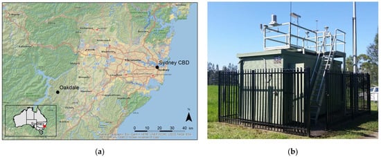
Figure 1.
Location of Oakdale (a) and the monitoring compound (looking NE) (b).
West of the station is the world-heritage-listed Greater Blue Mountains region (10,300 km2), including the Blue Mountains, Nattai and Kanangra-Boyd National Parks. Emissions from this sector (Blue Mountains, Oberon, Upper Lachlan areas) are totally dominated by natural emissions (92% or 17.8 kt p.a. VOC and 75% or 2.7 kt p.a. NOx) (https://www.epa.nsw.gov.au/your-environment/air/air-emissions-inventory, accessed: 10 August 2022).
There are coal-fired power stations WNW of the station. Mt Piper power station is a 1400 MW station with two boilers. It is approx. 88 km WNW of Oakdale. Wallerawang power station was a 1000 MW station with two units located approx. 82 km WNW of Oakdale. Wallerawang operated from 1957 to April 2014. Both stations have operated with low-NOx burners since 1993. In 2013, these stations together emitted 38.0 kt NOx, while in 2021, Mt Piper emitted 18.0 kt (https://www.dcceew.gov.au/environment/protection/npi, accessed: 10 August 2022).
East of the station is the Sydney Basin, with a population of 5.2 million people. Sydney’s basin topography and coastal setting can trap air pollution under certain synoptic—local meteorological configurations. Katabatic flow drains from the Blue Mountains towards the coast, accumulating emissions. Sea breezes can then transport this contaminated air mass back over urban areas where fresh emissions are added. This local land–sea circulation may persist for several days at times, especially when coincident with certain synoptic conditions such as a high-pressure system centred in the Tasman Sea [22,23].
The predominant wind in Oakdale is westerly or south-westerly in all seasons except summer (Figure 2). In summer, the regional sea breeze circulation predominates, transporting pollutants from the eastern part of the basin to Oakdale.
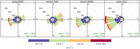
Figure 2.
Seasonal wind roses. Note predominant winds of westerly drainage flows in cooler months and ENE sea-breeze in summer.
The estimated population within 25 km of the station is approximately 100,000 people (>99% of those in the eastern sector); within 10 km, the population is ~6000. The TOAR database (https://join.fz-juelich.de, accessed: 10 September 2022 [20]) assesses nearby (25 km radius) land use categories as evergreen broadleaf forest 64.7%, woody savannas 17.6%, grasslands 6.4%, croplands: 5.1%, cropland/natural vegetation mosaic 2.3%, water 1.2%, and urban and built-up 1.0%.
2.2. Instrumentation, Calibration, and Maintenance
Monitoring at Oakdale commenced in April 1996, with continuous data collection for ozone, nitrogen oxides (NO, NO2, NOx), particles (PM10-TEOM, nephelometer), and meteorology (temperature, relative humidity, wind). Ozone is measured by ultraviolet (254 nm) photometry (TEI 49C, EC9810, API T400). NOx is measured by chemiluminescence with molybdenum converter (TEI 42C, EC9841, API T200). Instrument sets have been swapped at times (Table 1), with instrument exchanges occurring after prolonged inter-comparison studies at other sites showed no statistically significant difference between instrument types.

Table 1.
Instrument details for ozone and NOx measurements.
The glass manifold sampling inlet is at 3 m height and samples air continuously via a blower pump. Individual instruments draw air from the manifold through 0.635 mm Teflon/PTFE tubing using their internal pumps (flow rate 0.5 lpm). This sample tubing is ~0.5 m in length, resulting in a residence time within the PTFE sample line of ~2 s. Particle filters (47 mm, 5 μm) in line with the tubing remove particles prior to entering the instrument; each instrument also has a second internal particle filter that removes any residual particles.
Ozone calibrations comply with Australia Standard AS/NZS 3580.6.1 and are consistent with the WMO Guidelines for Continuous Measurements of Ozone in the Troposphere (https://library.wmo.int/doc_num.php?explnum_id=7814, accessed: 10 October 2022). Initial instrument calibrations occur at commissioning and after all major maintenance activities. Calibration checks occur at 0, 50, 100, 200, and 400 ppb. Audits/calibrations occur every 6 months using the same check points.
Zero- and single-point checks occur daily at 01:00 AEST. For the NOx instrument, NIST traceable gas (NO) in a multi-component mix is diluted with zero air and provided at known concentration. Ozone is generated on-site at a specific concentration and, after a short period of NO measurement, is introduced to the NOx instrument, forming NO2 at a known concentration and assessing instrument gas-phase-titration and converter efficiency. The generated ozone is simultaneously introduced to the ozone instrument. Ozone measurements and generation are traceable to Standard Reference Photometer (SRP-21) [26] through transfer standards (Dasibi 1008 (Glendale, CA, USA), Tanabyte T724 (Riverview, FL, USA)).
While three different instrument makes (Table 1) have been used to measure ozone during the study period, they are consistent in their measurement technique. All instruments use UV photometry (254 nm), identical sampling systems and identical calibration systems (all traceable to primary standard NIST SRP-21). Further, when changing instrument types in our network, a detailed inter-comparison is first undertaken. We, therefore, conclude that there is little chance of instrument-specific biases in our analysis.
Routine instrument maintenance complies with relevant Australia Standards (AS/NZS 3580.1.1—Station Siting, AS/NZS 3580.5.1—NOx, AS/NZS 3580.6.1—Ozone, AS/NZS 3580.14—Meteorology). Monthly maintenance includes cleaning and inspection of the sample system, leak checking and replacing inline particle filters; six monthly maintenance includes sample line cleaning, replacing internal particle filters, and UV lamp and scrubber efficiency tests; annual maintenance includes cleaning of reaction cells, replacement of scrubbers, and servicing of all sample pumps.
2.3. Data Handling
Data validation is AS/NZS 3580.19 compliant. Further, data is included in our analysis when it meets the 75% data availability criteria set for demonstrating Australian National Environment Protection Measure reporting [27]. That is, valid hourly averages require at least 75% of 1 min average data to be valid, and valid 8-hour averages require at least 75% of hourly values in the period to be valid. A daily summary is reported when 75% of hourly samples in the day are valid, and a yearly summary is provided when 75% of days in the year are valid and each calendar quarter has 75% valid days. These acceptance tests are extended in our analysis to include a valid season where 75% of days in the season are valid (note here we are discussing austral seasons, that is: summer (December–February), autumn (March–May), winter (June–August), spring (September–November)).
The daily span and zero tests for the ozone and NOx instruments result in lost hours. Gaps due to these tests are typically 1 h but may be 2 h long prior to 1999 due to a longer time allocated for the zero/span check initially. These gaps are filled by averaging the hours on either side of the missing value if each hour is valid.
Data capture rates are typically high; however, there have been some extended periods of missing ozone data due to various reasons (Figure 3). Of most note is data excluded from April 2001 to October 2002 due to issues with power supply and questionable performance of the monitor due to potential issues with sample tubing.
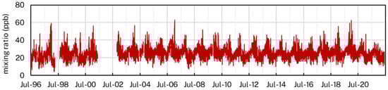
Figure 3.
Daily average 1 h ozone showing data capture. Note: Missing data from April 2001 to October 2002.
Valid hourly ozone data were available for 94% of the period (24,637 valid hours). This provided summary datasets with 8315 (89%) valid days, 264 valid months (85%) and 83 valid seasons (80%).
VOCs at high concentrations can interfere with ozone measured using UV photometry [28]. All ozone instruments used at Oakdale have operated with solid manganese dioxide catalytic scrubbers; hence our measurements are susceptible to interferences from VOCs at high concentrations. There are very few anthropogenic sources of VOCs in the vicinity; however, within smoke plumes, VOC levels can be large and may impact the ozone measurements. To minimise these impacts on our analysis, we exclude periods impacted by smoke events from bushfires or hazard reduction burning. We do this by excluding data from the analysis where coincident nephelometer measurements are high (bsp > 2.1 Mm−1), a strong marker of bushfire/hazard reduction burning smoke.
Commercial NOx monitors can see interferences from reactive nitrogen species such as nitric acid (HNO3), nitrous acid (HONO), nitric acid anhydride (N2O5), ammonia (NH3), alkyl nitrates (RONO2), peroxyacetyl nitrates (PAN) and nitrate aerosols [29]. The NOx we report here is more accurately NOy = NO + NO2 + NOz, where NOz = HNO3 + HONO + N2O5 + RONO2 + PAN + other N species.
2.4. Identifying Background Ozone
Background ozone can be defined in several ways: policy-relevant (US EPA), baseline [30], night-time [25], day-time [31] and warm-season [32]. An extensive overview of the different terms and approaches to calculating background is found in [30].
In this study, we interpret background ozone similarly to [33], where principal component analysis is used to assess baseline ozone across 97 non-urban sites in North America. Recently, [15] applied k-means clustering (analogous to principal component analysis from [33]) to identify background ozone in Gunnedah, Australia.
The k-means algorithm is an iterative clustering process that groups together data with similar characteristics, here ozone and meteorology. Initially, k points are randomly chosen from the observation set. These points act as centroids for each k cluster. Observations are then assigned to the group of the closest centroid (based on standardised Euclidean distance). Once all observations have been assigned to a group, new k centroids are chosen and the process is repeated until convergence, i.e., the centroids do not move, and the standardised Euclidean distance within the groups is minimised. We implement the algorithm within the open-air R package v2.10-0 [34,35].
The method identifies clusters of observations where local emissions are minimised, and the background ozone contributions are at their maximum. Here, we use the term “background ozone” to refer to the regional background, that is, ozone levels that are typically representative of a broad region and that are little influenced by anthropogenic emissions within the region.
2.5. Trend Identification and Quantification
The standard non-parametric Mann–Kendall (M-K) test for trend is appropriate and well-suited to test the presence of trend in the air quality summary statistics data. It is simple, robust, does not require prior knowledge of the ozone distribution and has been used extensively in the air quality literature. M-K tests whether data series with time (x versus t) tend to increase or decrease (i.e., monotonic change) [36].
If a statistically significant trend was found, the slope of the trend was estimated using Sen’s non-parametric method [36].
3. Results
We commence by describing the full ozone record at the site, including analysis of seasonal, weekday and diurnal variations. To assist in interpretation, we break the data into four periods, 1996/97–2002/03, 2002/03–2010/11, 2010/11–2017/18 and 2017/18–2021/22, noting that the first period covers five years of data only due to missing data. Seven-year periods are selected to approximate the long-term frequency of central Pacific El-Nino events found by [37], i.e., approximately four events per 30 years. We note, however, that while this choice is based on the physical climate and is supported through previous work on synoptic classification in Eastern Australia [23,38], our temporal sub-setting is somewhat arbitrary, as the main goal is simply to assist in analysis and investigation of the results.
We also assess for trends in the full ozone, NO2, NO and OX datasets to assess overall photochemical characteristics at the site. Trend analysis includes annual averages, daily maxima and quantiles (median, 25th, 75th and 95th percentiles).
3.1. Annual, Seasonal, Day-of-Week and Diurnal Variations
Over the entire observation set, the mean ozone mixing ratio was 25.2 ppb. Annual (July–June) mean anomalies, that is, the variation of the annual mean from the mean of the full observational period (1996–2022), vary from −4.0 ppb in 1996/97 through to +3.4 ppb in 2006/07. Anomalies broadly coincide with the El Niño-Southern Oscillation, with typically below-average concentrations during La Niña years and higher than average during El Niño events as classified by the Oceanic Niño Index (Figure 4).
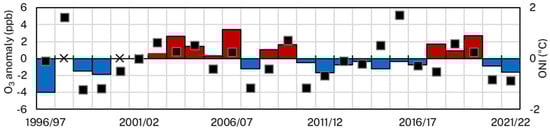
Figure 4.
Annual mean ozone anomalies (base 1996–2022, bars with missing data marked ×) showing years above (red) and below (blue) long term mean, and the Oceanic Niño Index (ONI, black squares, https://psl.noaa.gov/data/correlation/oni.data).
Diurnal ozone profiles were similar across all periods but with some variation. Peak ozone is typically observed between 1200–1800 with mean concentrations of 31.3 ppb and minimum concentrations mid-morning 00:00–08:00 (20.8 ppb). Lower night-time concentrations were observed during 1996–2003 (18.9 ppb), while day-time concentrations in that period were comparable to recent years. Higher day-time peak concentrations were seen during 2003–2010 (32.7 ppb) (Table 2).
Table 2.
Summary of mean ozone, NO2 and NO mixing ratios (ppb) for all observations.
There is little variation in ozone concentrations throughout the week; however, there is some indication of a weekend effect in the early years of the record (Figure 5b). We observe 1996–2003 showing a statistically significant weekend effect (based on the overlap of the 95% confidence intervals in the mean). Between 1996–2022 mean weekday ozone was 25.0 ppb, while mean weekend concentrations were 25.6 ppb. The insignificant weekday/weekend effect implies that local anthropogenic emissions do not vary significantly from day to day.
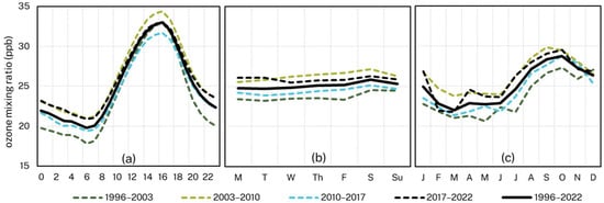
Figure 5.
Summary of diurnal (a), weekly (b) and monthly (c) ozone mean mixing ratios.
Seasonal variations show higher ozone concentrations from August to December (mean 27.6 ppb). A springtime peak is evident in September–October (28.6 ppb) across all periods. The mean difference between the springtime peak and the autumn minima (MAM) was 5.6 ppb and ranged from 5.1 ppb (2003–2010) to 6.2 ppb (2010–2017).
Observed NO2 concentrations are typically very low. This is not unexpected, given the emissions profiles of the surrounding region. Across all available data, mean NO2 concentrations were 2.0 ppb. Analysis of the weekday and diurnal NO2 profiles (Figure 6) show only small variations in monthly concentrations, with maxima in December–January (2.5 ppb) and minima in June–August (1.3 ppb). There is little weekday/weekend variation in NO2, with weekday mean concentrations (2.1 ppb) slightly higher than weekends (1.7 ppb). Diurnal profiles show a peak in the evening. Together with slightly higher concentrations in summer and during the week, this implies that the evening peak may be due to the transport of air from the Sydney Basin during sea breeze events. NO concentrations are near zero for much of the study, demonstrating the aged nature of the airmasses at this station and the limited contribution of fresh local NOx emissions.
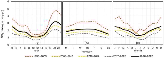
Figure 6.
Summary of (a) diurnal, (b) weekly and (c) monthly NO2 mean mixing ratios.
NO2 concentrations are notably higher in the 1996–2003 period (Table 2). This may be due to the higher NOx emissions in the Sydney Basin prior to the banning of leaded petrol and the introduction of US’90 (1999) and EURO 2 (2004) vehicle emissions standards. NO2 concentrations continue to fall as motor vehicle NOx emissions decline. It may also reflect some contributions early in the record from distant power stations.
3.2. Identifying a Background Cluster
The EU Directive supports the assessment of background ozone in the vicinity of an urban conglomeration if it is sited upwind of the urban area. The complex topography of the Sydney Basin and its coastal location means that identifying stations that are purely upwind of the city is difficult due to synoptic and mesoscale processes within the region. For example, at Oakdale, regional westerly to south-westerly flows dominate in winter leading to a clear designation as an upwind site. In contrast, during summer, the sea-breeze/land-breeze circulation means that Oakdale is both upwind and downwind of the city, depending on the predominant synoptic conditions and the time of day.
We categorise ozone in Oakdale into several clusters using k-means clustering. This is comparable to the clustering of back trajectories but using local wind speed, wind direction and concentrations to group similar conditions rather than air mass origins [39]. We substitute k-means clusters for the principal components used by [33] and test clustering with 3 ≤ k ≤ 8 (Figure 7). We identify a cluster of ozone in the sector of ~235°–325° with wind speeds >~2 ms−1 and associated with low NO2 (Figure 8). Many observations in this cluster are assigned to the same cluster irrespective of the chosen k value. We hence assess optimal clustering for background ozone at k = 4.
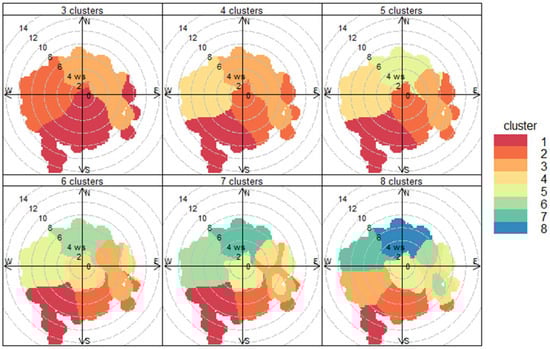
Figure 7.
Results for k-means cluster analysis for 3 ≤ k < 8.
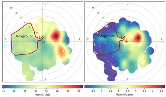
Figure 8.
Ozone and NO2 mean mixing ratios within the background cluster.
Table 3 summarises the mean ozone and NO2 mixing ratios for each cluster (k = 4). The mean O3 in the background cluster (Cluster 4) is 25.9 ppb. The mean warm season (October–March) ozone in the background cluster is 27.2 ppb, while the mean warm season NO2 in the background cluster is 1.3 ppb.
Table 3.
Mean mixing ratios (ppb) for each cluster.
We also identify a cluster (no. 3) that has higher O3 and NO2 than the background cluster. The mean warm season (2.6 ppb) and annual (2.5 ppb) NO2 are higher here than in the background cluster (1.3 and 0.9 ppb, respectively). Warm season (35.9 ppb) and annual (34.5 ppb) O3 in this cluster are much greater than the background. Cluster 3 represents the transport of air masses from the Sydney Basin, particularly in the warm season under NNE sea breeze events. There is some variation within the background cluster through the period (Table 4). There is a lower number of observations in the background cluster for 2017–2022 due to fewer years and screening out of significant amounts of data due to bushfires (September 2019–February 2020) and hazard reduction burns.
Table 4.
Mean mixing ratios (ppb) within the cluster identified as representing regional background.
Within the background cluster, there is little variation in ozone concentrations throughout the week. Diurnal variations are evident, but their amplitude is lower compared to the entire observational dataset. The seasonal signal of the background cluster is like the overall dataset, with ozone maxima in September–October and minima in March–May (Figure 9).
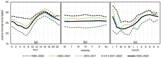
Figure 9.
Diurnal (a), weekly (b) and monthly (c) background ozone mean mixing ratios.
3.3. Trends in Background Ozone
Following the identification of a cluster of measurements likely representative of background air masses, we test for any trends and their significance. Firstly, we summarize the annual (July–June) hourly ozone measurements within the background cluster. Figure 10 shows the distribution of hourly measured background ozone. Here, we plot the interquartile range (box), the median (dash within the box) and the mean (red square) and represent the 5th and 95th percentiles as the upper and lower whiskers. The lines show significant trends (M-K test, α = 0.05) in the 5th and 95th percentiles and the annual mean.
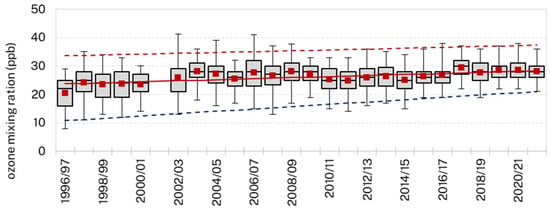
Figure 10.
Distribution of hourly mean background ozone mixing ratios. Boxes represent the interquartile range, square marker is the mean, line is the median, whiskers are 5th and 95th percentiles and dashed lines are their linear trends from Sen’s estimate (Table 5).
We apply the M-K test for monotonic change on the annual statistics for the background ozone distribution. If a significant trend (at α = 0.05) is identified, we use the Sen estimator to quantify that trend. Table 5 summarises the trend analysis. We find significant increasing trends in the 5th, 25th, 50th (median) and 75th percentiles, the annual mean, and the annual standard deviation of background ozone. We also find that the trend in the 95th percentile is significant if we set α = 0.1. There is no significant trend in the annual maximum 1 h background ozone at the 0.1 significance level.
Table 5.
Annual trends in distribution statistics of hourly background O3 and NO2. Significance at different α values: 0.01 ***, 0.02 **, 0.05 *, 0.1 +, no significance ---.
The distribution of background ozone is narrowing, with the standard deviation of hourly ozone declining by 0.8 (0.4–1.2) ppb per decade. Much of this trend is seen through greater increases in the lower end of the distribution rather than in peak ozone concentrations. The 5th percentile is increasing at 4.1 (2.9–5.3) ppb per decade, and the 25th percentile at 2.5 (1.4–3.6) ppb per decade, while the 95th percentile is increasing at 1.5 (0.0–3.1) ppb/decade, and there is no significant trend in annual maximums. The mean annual background ozone in Oakdale is increasing by 1.8 (1.0–2.8) ppb/decade.
Even though NOx emissions from the background sector are low, they are non-trivial, particularly in the early years of the record. Assessment of the annual distribution of NO2 mixing ratios identifies several aspects that can help explain some of the observed increases in background ozone. The M-K test identifies statistically significant reductions in annual maximum, mean, median, standard deviation and the 95th and 75th percentiles. No trend was found in the 5th and 25th percentiles, as these are near zero throughout the record. While there is a statistically significant decline in annual mean background NO2 mixing ratios 0.6 (0.5–0.7) ppb/decade, we note that this represents a minimal overall decline in terms of ppb. Annual 1 h maxima have declined by 5.8 (4.4–8.2) ppb per decade, while the 95th percentile of observations is declining by 1.7 (1.3–2.1) ppb/decade (Figure 11). These significant declines in the higher NO2 mixing ratios within the background air may signify that earlier in the record, emissions from the distant power stations may be identifiable within the background cluster.
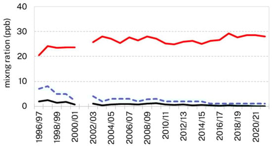
Figure 11.
Annual mean ozone (red), NO2 (black) and 95th percentile of NO2 (blue dashed) in background air.
We hypothesize that some of the increases in background ozone are likely due to reduced NOx emissions from distant power stations and, more broadly, from lower motor vehicle emissions in the wider region. As the airmasses at this location are almost universally NOx limited, any reduction in NOx will lead to reductions in ozone. From 2004 onwards, mean NO2 mixing ratios in background air have been <1.2 ppb, and the 95th percentile of hourly NO2 measurements have been <3.0 ppb. From 2014 (the Wallerawang power station’s closure), the mean NO2 is 0.3 ppb, and the 95th percentile is 1.1 ppb. Hence, while there still may be some contribution from the power station sources, this contribution is diminishing.
4. Discussion
Expanding on the work of [15], we use k-means clustering on a long-term dataset from Oakdale, NSW, to identify a measurement cluster that likely represents background air in Eastern Australia of continental origin. The cluster is characterised by winds from the SW-NW sector, with wind speeds > 2 ms−1 and associated low NO2. Early in the record, we observed higher peak NO2 measurements within the cluster and attributed this to some transport of emissions from distant power stations (~82 km to the NNW). Emissions from these power stations declined significantly from 2014, and now mean NO2 concentrations in the background cluster are ~0.2 ppb, indicating little impact of local NOx emissions.
Focusing on the most recent period (2017–2022), we find annual mean background ozone of 28.5 ppb. We find a statistically significant (α = 0.05) trend in the mean of +1.8 (1.0–2.8) ppb/decade. Within the background cluster, there is no attributable weekday/weekend effect. There is some variation in the diurnal signal (amplitude of 4 ppb) and some seasonality with minima observed in the Austral autumn (March–May).
These estimates are close to those from other published background ozone results in Australia (e.g., Gape Grim 25 ppb, Latrobe Valley 21–29 ppb, Manjimup 19 ppb, Ovens 17 ppb) but lower than recent observations from Gunnedah (36–39 ppb). Our results do not support previous conclusions on background ozone in Australia of 45 ppb [40].
Our trend analysis shows that the distribution of background ozone in Oakdale is narrowing, driven by greater increases in the lower end of the distribution rather than in peak ozone concentrations. The 5th, 25th and 95th percentiles are all increasing but at differing rates (4.1, 2.5, 1.5 ppb/decade, respectively). The mean annual background ozone in Oakdale is increasing by 1.8 (1.0–2.8) ppb/decade.
In contrast, using TOAR data [41] finds that in the Southern Hemisphere, there is little evidence for an increase in ozone from the historical to the modern period. Focusing on recent trends at baseline Southern Hemisphere sites, significant trends in ozone in Cape Grim (0.6 ppb/decade, 1982–2010), Cape Point (1.9 ppb/decade, 1983–2011) and Arrival Heights (2.9 ppb/decade, 1997–2008) have been found [42]. Our results fit within these findings.
The night-time background ozone trend reported in Western Sydney of 4.3 ppb/decade, based on data from 1998 to 2005 [25], is significantly higher than our assessment of 1.8 ppb/decade for background air at Oakdale.
Further investigation of the chemical composition of Australian continental air masses is required to better contextualise our results.
Relevance to the Global Atmosphere Watch Program
Our results suggest that the Oakdale station, and stations with similar characteristics, can provide additional valuable information on regional atmospheric composition.
The GAW mission statement [43] highlights the multiple benefits that a better understanding of background tropospheric ozone can provide. While the GAW networks provide critical information on global and regional tropospheric ozone, within Australia, the only long-term monitoring for GAW reactive gases [44] is from Cape Grim, a baseline station focused on the Southern Ocean marine environment. There are no GAW stations in Australia that focus on regional background reactive gases. The GAW Reactive Gases Scientific Advisory Group (SAG) has acknowledged this gap in the Southern Hemisphere.
In this study, we have attempted to use the unique siting and regional characteristics of the Oakdale station to identify background air parcels and then estimate the concentrations of key reactive gases ozone and NO2. Oakdale is a long-term station that is well-sited and is operated under a rigorous, documented and audited quality assurance program [45]. Ozone measurements from Oakdale are directly traceable to SRP21 and NO/NO2 measurements to SRP21 and NIST-certified standards. We have used these characteristics and statistical methods to identify a background sector for Oakdale that would likely adhere to GAW requirements for a regional station.
More formally assessing GAW requirements for regional stations [46], Oakdale meets the following:
- It is regionally representative and is normally free of the influence of significant local pollution sources or at least frequently experiences an advection of pollution-free air from specific wind directions. We use k-means clustering to identify a regional background signal that occurs 24% of the time. Within this cluster, we show that NO titration from local emissions is low (mean NO2 < 1.2 ppb and since 2014, mean NO2 ≤ 0.3 ppb);
- A commitment by the responsible agency to long-term observations of at least two variables in at least one GAW focal area. Oakdale has operated since 1996 and is a core component of the NSW AQMN and its ongoing plan. Oakdale monitors reactive gases (O3, NOx), aerosols (PM2.5 mass, PM10 mass, light scattering) and UV radiation;
- Greater than 90% data capture. Since 2002 data recovery rates have been >96%;
- Standard meteorological in situ observations. Temperature, relative humidity, horizontal wind and pressure are measured at the station.
Additionally, the GAW QA requirements are also met, and the network that Oakdale is part of is independently accredited by the National Association of Testing Authorities. Currently, data from Oakdale are available through the TOAR database [20] (https://toar-data.org/, accessed: 10 October 2022) and the NSW air quality data services (https://www.dpie.nsw.gov.au/air-quality/air-quality-data-services, accessed: 10 October 2022).
Our assessment here demonstrates that measurements from regional and national air quality monitoring networks can readily supplement the GAW networks. We encourage jurisdictional air quality monitoring network operators to consider integrating their measurements of reactive gases into the GAW. Doing so can assist in filling gaps in under-sampled regions such as the Southern Hemisphere.
Author Contributions
Conceptualization, M.L.R. and N.J.; methodology, M.L.R. and N.J.; formal analysis: M.L.R.; resources, M.L.R. and N.J.; data curation, M.L.R.; writing—original draft, M.L.R., N.J., H.N.D. and M.A.; writing—review and editing, M.L.R., N.J., H.N.D. and M.A.; funding acquisition, M.L.R. All authors have read and agreed to the published version of the manuscript.
Funding
This research received no external funding.
Data Availability Statement
All air quality data presented here are freely and openly available from the New South Wales Government’s Air Quality Data Services (https://www.dpie.nsw.gov.au/air-quality/air-quality-data-services, accessed: 10 October 2022).
Acknowledgments
We acknowledge the work of DPE technicians in maintaining the Oakdale monitoring station, including B. White, D. Hill, L. Jenson, J. Kirkwood, G. Ross, S. Serdar and many others over the years. The Oakdale station is on the traditional lands of the Dharug nation, and we acknowledge their elders, past, present and emerging.
Conflicts of Interest
The authors declare that they have no known competing financial interest or personal relationship that could have influenced the work reported in this paper.
References
- Nicolas, M.; Ramalho, O.; Maupetit, F. Reactions between ozone and building products: Impact on primary and secondary emissions. Atmos. Environ. 2007, 41, 3129–3138. [Google Scholar] [CrossRef]
- Manisalidis, I.; Stavropoulou, E.; Stavropoulos, A.; Bezirtzoglou, E. Environmental and health impacts of air pollution: A review. Front. Public Health 2020, 8, 14. [Google Scholar] [CrossRef]
- Stevens, C.J.; Bell, J.N.B.; Brimblecombe, P.; Clark, C.M.; Dise, N.B.; Fowler, D.; Lovett, G.M.; Wolseley, P.A. The impact of air pollution on terrestrial managed and natural vegetation. Philos. Trans. R. Soc. A 2020, 378, 20190317. [Google Scholar] [CrossRef] [PubMed]
- Jaffe, D.A.; Wigder, N.L. Ozone production from wildfires: A critical review. Atmos. Environ. 2012, 51, 1–10. [Google Scholar] [CrossRef]
- Clapp, L.J.; Jenkin, M.E. Analysis of the Relationship between Ambient Levels of O3, NO2 and NO as a Function of NOx in the UK. Atmos. Environ. 2001, 35, 6391–6405. [Google Scholar] [CrossRef]
- Fishman, J.; Solomon, S.; Crutzen, P.J. Observational and theoretical evidence in support of a significant in-situ photochemical source of tropospheric ozone. Tellus 1979, 31, 432–446. [Google Scholar] [CrossRef]
- Vingarzan, R. A review of surface ozone background levels and trends. Atmos. Environ. 2004, 38, 3431–3442. [Google Scholar] [CrossRef]
- Vecchi, R.; Valli, G. Assessment of ozone levels at alpine sites in Northern Italy. WIT Trans. Ecol. Environ. 1970, 28, 10. [Google Scholar]
- Cox, R.A.; Eggleton, A.E.J.; Derwent, R.G.; Lovelock, J.E.; Pack, D.H. Long-range transport of photochemical ozone in north-western Europe. Nature 1975, 255, 118–121. [Google Scholar] [CrossRef]
- Chatfield, R.; Harrison, H. Tropospheric ozone: 1. Evidence for higher background values. J. Geophys. Res. 1977, 82, 5965–5968. [Google Scholar] [CrossRef]
- Fishman, J.; Crutzen, P.J. The origin of ozone in the troposphere. Nature 1978, 274, 855–858. [Google Scholar] [CrossRef]
- Cooper, O.R.; Langford, A.O.; Parrish, D.D.; Fahey, D.W. Challenges of a lowered US ozone standard. Science 2015, 348, 1096–1097. [Google Scholar] [CrossRef]
- EPA 600/R-05/004aF; Air Quality Criteria for Ozone and Other Photochemical Oxidants. U.S. Environmental Protection Agency, Office of Air Quality Planning and Standards: Research Triangle Park, NC, USA, 2006; Volume I.
- European Union (EU). Directive 2002/3/EC of the European Parliament and of the Council relating to ozone in ambient air. Off. J. Eur. Communities 2002, L67, 14–30. [Google Scholar]
- Riley, M.L.; Watt, S.; Jiang, N. Tropospheric ozone measurements at a rural town in New South Wales, Australia. Atmos. Environ. 2022, 281, 119143. [Google Scholar] [CrossRef]
- West, J.J.; Naik, V.; Horowitz, L.W.; Fiore, A.M. Effect of regional precursor emission controls on long-range ozone transport–Part 1: Short-term changes in ozone air quality. Atmos. Chem. Phys. 2009, 9, 6077–6093. [Google Scholar] [CrossRef]
- Galbally, I.E.; Miller, A.J.; Hoy, R.D.; Ahmet, S.; Joynt, R.C.; Attwood, D. Surface ozone at rural sites in the Latrobe valley and Cape Grim, Australia. Atmos. Environ. 1986, 20, 2403–2422. [Google Scholar] [CrossRef]
- Reisen, F.; Meyer, C.P.; McCaw, L.; Powell, J.C.; Tolhurst, K.; Keywood, M.D.; Gras, J.L. Impact of smoke from biomass burning on air quality in rural communities in southern Australia. Atmos. Environ. 2011, 45, 3944–3953. [Google Scholar] [CrossRef]
- Ayers, G.P.; Penkett, S.A.; Gillett, R.W.; Bandy, B.; Galbally, I.E.; Meyer, C.P.; Elsworth, C.M.; Bentley, S.T.; Forgan, B.W. The annual cycle of peroxides and ozone in marine air at Cape Grim, Tasmania. J. Atmos. Chem. 1996, 23, 221–252. [Google Scholar] [CrossRef]
- Schultz, M.G.; Schroder, S.; Laypina, O.; Cooper, O.R.; Galbally, I.; Petropavlovskikh, I.; von Schneidemesser, E.; Tanimoto, H.; Elshorbany, Y.; Naja, M.; et al. Tropospheric Ozone Assessment Report: Database and metrics data of global surface ozone observations. Elem. Sci. Anthr. 2017, 5, 58. [Google Scholar] [CrossRef]
- Ahmet, S. Synoptic and mesoscale weather features associated with O3 and SO2 peaks in the Latrobe Valley. In Proceedings of the 8th International Clean Air Conference, Melbourne, VIC, Canada, 7–11 May 1984. Clean Air Society of Australia and New Zealand. Melbourne, Australia. [Google Scholar]
- Hart, M.; De Dear, R.; Hyde, R. A synoptic climatology of tropospheric ozone episodes in Sydney, Australia. Int. J. Climatol. A J. R. Meteorol. Soc. 2006, 26, 1635–1649. [Google Scholar] [CrossRef]
- Jiang, N.; Betts, A.; Riley, M.L. Summarising climate and air quality (ozone) data on self-organising maps: A Sydney case study. Environ. Monit. Assess. 2016, 108, 103. [Google Scholar] [CrossRef]
- Environment Protection Authority Victoria, Air Quality Monitoring Reports. Available online: https://www.epa.vic.gov.au/searchresults?q=air+monitoring+report (accessed on 17 May 2023).
- Duc, H.; Azzi, M.; Wahid, H.; Ha, Q.P. Background ozone level in the Sydney basin: Assessment and trend analysis. Int. J. Climatol. 2013, 33, 2298–2308. [Google Scholar] [CrossRef]
- Viallon, J.; Idrees, F.; Moussay, P.; Wielgosz, R.; Ross, G. Comparison of Ozone Reference Standards of the OEH and the BIPM, Feb 2020. BIPM-2020/01. Available online: https://www.bipm.org/documents/20126/27085544/RapportBIPM-2020-01.pdf/4c0100ec-915c-b53b-ce37-3f5a493754b9 (accessed on 10 October 2022).
- ISBN 978-1-921173-59-2; National Environment Protection Council (NEPC), 2011. Methodology for Setting Air Quality Standards in Australia. Part A. Available online: http://www.nepc.gov.au/system/files/resources/9947318f-af8c-0b24-d928-04e4d3a4b25c/files/aaqprctp04screeningprocedures200705final.pdf (accessed on 1 August 2021).
- Long, R.W.; Whitehill, A.; Habel, A.; Urbanski, S.; Halliday, H.; Colón, M.; Kaushik, S.; Landis, M.S. Comparison of ozone measurement methods in biomass burning smoke: An evaluation under field and laboratory conditions. Atmos. Meas. Tech. 2021, 14, 1783–1800. [Google Scholar] [CrossRef] [PubMed]
- Dickerson, R.R.; Anderson, D.C.; Ren, X. On the use of data from commercial NOx analyzers for air pollution studies. Atmos. Environ. 2019, 214, 116873. [Google Scholar] [CrossRef]
- McDonald-Buller, E.C.; Allen, D.T.; Brown, N.; Jacob, D.J.; Jaffe, D.; Kolb, C.E.; Lefohn, A.S.; Oltmans, S.; Parrish, D.D.; Yarwood, G.; et al. Establishing policy relevant background (PRB) ozone concentrations in the United States. Environ. Sci. Technol. 2011, 45, 9484–9497. [Google Scholar] [CrossRef]
- Parrish, D.D.; Fahey, D.W.; Williams, E.J.; Liu, S.C.; Trainer, M.; Murphy, P.C.; Albritton, D.L.; Fehsenfeld, F.C. Background ozone and anthropogenic ozone enhancement at Niwot Ridge, Colorado. J. Atmos. Chem. 1986, 4, 63–80. [Google Scholar] [CrossRef]
- Dolwick, P.; Akhtar, F.; Baker, K.R.; Possiel, N.; Simon, H.; Tonnesen, G. Comparison of background ozone estimates over the western United States based on two separate model methodologies. Atmos. Environ. 2015, 109, 282–296. [Google Scholar] [CrossRef]
- Chan, E.; Vet, R.J. Baseline levels and trends of ground level ozone in Canada and the United States. Atmos. Chem. Phys. 2010, 10, 8629–8647. [Google Scholar] [CrossRef]
- Carslaw, D.C.; Ropkins, K. Openair—An R package for air quality data analysis. Environ. Model. Softw. 2012, 27, 52–61. [Google Scholar] [CrossRef]
- Carslaw, D.C. The Openair Manual—Open-Source Tools for Analysing Air Pollution Data; Manual for Version 1.1-4; King’s College London: London, UK, 2015. [Google Scholar]
- Salmi, T.; Määttä, A.; Anttila, P.; Ruoho-Airola, T.; Amnell, T. Detecting Trends of Annual Values of Atmospheric Pollutants by the Mann-Kendall Test and Sen’s Slope Estimates MAKESENS–The Excel Template Application; Finish Meteorological Institute: Helsinki, Finland, 2002. [Google Scholar]
- Freund, M.B.; Henley, B.J.; Karoly, D.J.; McGregor, H.V.; Abram, N.J.; Dommenget, D. Higher frequency of Central Pacific El Niño events in recent decades relative to past centuries. Nat. Geosci. 2019, 12, 450–455. [Google Scholar] [CrossRef]
- Jiang, N.; Cheung, K.; Luo, K.; Beggs, P.J.; Zhou, W. On two different objective procedures for classifying synoptic weather types over east Australia. Int. J. Climatol. 2012, 32, 1475–1494. [Google Scholar] [CrossRef]
- Carslaw, D.C.; Beevers, S.D. Characterising and understanding emission sources using bivariate polar plots and k-means clustering. Environ. Model. Softw. 2013, 40, 325–329. [Google Scholar] [CrossRef]
- Physick, B.; Edwards, M.; Cope, M. A Screening Procedure for Monitoring Ozone and Nitrogen Dioxide in “Small-to Medium-Sized” Cities: Phase II-Application of the Procedure; CSIRO Atmospheric Research: Aspendale, Australia, 2002. [Google Scholar]
- Tarasick, D.; Galbally, I.E.; Cooper, O.R.; Schultz, M.G.; Ancellet, G.; Leblanc, T.; Wallington, T.J.; Ziemke, J.; Liu, X.; Steinbacher, M.; et al. Tropospheric Ozone Assessment Report: Tropospheric ozone from 1877 to 2016, observed levels, trends and uncertainties. Elem. Sci. Anthr. 2019, 7, 39. [Google Scholar] [CrossRef]
- Cooper, O.R.; Schultz, M.G.; Schröder, S.; Chang, K.L.; Gaudel, A.; Benítez, G.C.; Cuevas, E.; Fröhlich, M.; Galbally, I.E.; Molloy, S.; et al. Multi-decadal surface ozone trends at globally distributed remote locations. Elem. Sci. Anthr. 2020, 8, 23. [Google Scholar] [CrossRef]
- WMO. WMO Global Atmosphere Watch (GAW) Implementation Plan: 2016–2023; GAW Report No. 228; World Meteorological Organization: Geneva, Switzerland, 2017; ISBN 978-92-63-11156-2. [Google Scholar]
- Schultz, M.G.; Akimoto, H.; Bottenheim, J.; Buchmann, B.; Galbally, I.E.; Gilge, S.; Helmig, D.; Koide, H.; Lewis, A.C.; Novelli, P.C.; et al. The Global Atmosphere Watch reactive gases measurement network. Elem. Sci. Anthr. 2015, 3, 67. [Google Scholar] [CrossRef]
- Riley, M.; Kirkwood, J.; Jiang, N.; Ross, G.; Scorgie, Y. Air quality monitoring in NSW: From long term trend monitoring to integrated urban services. Air Qual. Clim. Chang. 2020, 54, 44–51. [Google Scholar]
- WMO. Guidelines for Continuous Measurements of Ozone in the Troposphere; GAW Report No. 209; World Meteorological Organization: Geneva, Switzerland, 2013; ISBN 978-92-63-11110-4. [Google Scholar]
Disclaimer/Publisher’s Note: The statements, opinions and data contained in all publications are solely those of the individual author(s) and contributor(s) and not of MDPI and/or the editor(s). MDPI and/or the editor(s) disclaim responsibility for any injury to people or property resulting from any ideas, methods, instructions or products referred to in the content. |
© 2023 by the authors. Licensee MDPI, Basel, Switzerland. This article is an open access article distributed under the terms and conditions of the Creative Commons Attribution (CC BY) license (https://creativecommons.org/licenses/by/4.0/).