Article

Triggering of an Epidemic Outbreak via Long-Range Atmospheric Transport of Bio-Aerosols—Application to a Hypothetical Case for COVID-19

1
Rowe Consulting, 22 Chemin des Moines, 22750 Saint Jacut de la Mer, France
2
MERL-Consulting SAS, 21 Rue Sergent Guihard, 35000 Rennes, France
3
CNRS (Centre National de la Recherche Scientifique), IPR (Institut de Physique de Rennes)-UMR 6251, Université de Rennes, 35000 Rennes, France
4
Meteozone Consulting, Rockville, MD 20854, USA
*
Author to whom correspondence should be addressed.
Atmosphere 2023, 14(6), 1050; https://doi.org/10.3390/atmos14061050
Submission received: 26 April 2023 / Revised: 31 May 2023 / Accepted: 12 June 2023 / Published: 19 June 2023
(This article belongs to the Special Issue Aerobiology and Health Impacts)

Abstract

:
In the present work, we investigate the possibility that long-range airborne transport of infectious aerosols could initiate an epidemic outbreak at distances downwind beyond one hundred kilometers. For this, we have developed a simple atmospheric transport box model, which, for a hypothetical case of a COVID-19 outbreak, was compared to a more sophisticated three-dimensional transport-dispersion model (HYSPLIT) calculation. Coupled with an extended Wells–Riley description of infection airborne spread, it shows that the very low probability of outdoor transmission can be compensated for by high numbers and densities of infected and susceptible people in the source upwind and in the target downwind, respectively, such as occur in large urban areas. This may result in the creation of a few primary cases. It is worth pointing out that the probability of being infected remains very small at the individual level. Therefore, this process alone, which depends on population sizes, geography, seasonality, and meteorology, can only “trigger” an epidemic, which could then spread via the standard infection routes.

1. Introduction

The problem of epidemic outbreaks is central to the epidemiology of infectious diseases. It is expected that the understanding of the origins of an outbreak could allow further such events to be circumvented [1,2]. A famous example is the tracking of a cholera outbreak to a specific reservoir in London during the year 1854, demonstrating that cholera was transmitted through infected water [3]. Following this finding, it was clear that avoiding contaminated water and providing the population with safe drinking water was an essential requirement in fighting cholera. For disease that spreads from human to human, it is important therefore, to identify the first cases of illness outbreak, referred to as primary cases [1]. The very first case is quite often called “patient zero”, also for a zoonosis, but the hunt for primary cases or patient zero has proven to be difficult: examples are the case of the recent COVID-19 pandemic [4,5] or in the early 1980s, the HIV pandemic for which the primary case was never found [1] despite erroneous affirmations to the contrary.
Indeed, once a disease has spread, the hunt for “patient zero” is of less importance. The question becomes understanding how infectious diseases can be transmitted, in order to use mitigation measures that could hinder the development of an epidemic and to avoid the emergence of new pathogens. The COVID-19 pandemic has shown that, even nowadays, the question of mode of transmission for a new infectious disease can involve fierce discussions [6,7,8,9,10,11]. The main problem here was to know if contamination occurs principally through the transport of large droplets, which behave in a ballistic way (with impact on mucosa), or inhalation of bio-aerosols emitted by infected persons. In the latter case, the microdroplets have a sufficiently small size so as to linger in air for a very long time. The denial of this second method of transmission, including by international health authorities, led prominent researchers in the field to raise an alarm both in the scientific literature [12] and mainstream press [13].
The purpose of the present paper is to investigate the possibility of a long-distance wind-borne bio-aerosol route for the passage of a human pathogen from one region to another, leading to the creation of a very few primary cases that could serve as triggers for an epidemic in a new region. Such a possibility is quite well known in veterinary science, as discussed in Section 2, but to our knowledge has not been suggested for human epidemics. The present investigation may then suggest that border controls (while certainly useful) could be largely insufficient to avoid the regional outbreak of any airborne epidemic.
The present paper is organized as follows. In Section 2 we comment on some well-known cases of the transport of aerosols (including some that are infectious) over very long distances. In Section 3, we establish a new model of outdoor pathogen transmission. As in a previous paper [14], we use a simple atmospheric box model based on air flows. This earlier work showed that the outdoor risk of being contaminated is generally several orders of magnitude less than that of indoors. The present investigation uses concepts developed by Wells [15], and our outdoor model is very close to the well-known model of Wells–Riley [16] for the probability of being infected by pathogens present in respired air. In Section 4, we apply the model to a specific, although hypothetical, case: the possible COVID-19 contamination in northern France from cases in southern England and London, especially with variants with high viral load such as the Delta form or the higher contagiousness of the Omicron variant. Note that our atmospheric box model is one of the earliest and simplest developed concepts in the field of atmospheric dispersion [17]. Nowadays there exist a large variety of dispersion models that use sophisticated numerical tools (see for instance the review by Khan and Hassan [18]). Therefore, in Section 5, we compare the results of our atmospheric box model to the three-dimensional Lagrangian transport-dispersion HYSPLIT model, one of the most established nowadays. We discuss the question of the outdoor virus lifetime, and we analyze our results in light of the problem of contamination by very low doses, as related to single-hit models [6,19,20,21,22].

2. Long-Distance Transport of Both Inert and Bio-Aerosols

Generally speaking, an aerosol is a collection of fine or very fine particles suspended in air. For a sufficiently small size (i.e., micrometric) the drag force is large compared to gravity [14,23], implying that the particle can stay suspended for a very long time in still air before settling. In fact, perfectly still air is rare since convection streams recirculate aerosols making their lifetimes extremely long, allowing their convective transport to be possible over very long distances outdoors (thousands of kilometers as discussed below). Note that the term “aerosol” is also used in the medical and pharmaceutical fields, amongst others, for the mixture of a substance with a propellant gas enclosed under pressure in a container and released as a spray, which could involve drops of larger size.
The first question, concerning the long-distance transmission of micron- and submicron-sized particles in the atmosphere, can be answered via experiments and modeling. Examples of long-distance transmission of particulate matter in the atmosphere include the transport of Saharan sand [24], plastic microparticles [25], soot particles (PM2.5) from biomass burnings [26], and pollen transport from eastern North America to Greenland ([27] and references therein). These phenomena are well studied and documented, and their importance has been evaluated. Except for pollen, these examples refer to non-biological, inert matter and are cited from the point of view of the coupling of observation and simulation to understand the modes and parameters associated with their transmission and to demonstrate that long-distance travel can give rise to physical effects from these particles. Aerosols containing biological matter either made of living or non-living components are usually named bio-aerosols.
Does this long-distance transmission of microparticles have relevance to the spread of diseases? What is the likelihood of biological matter, and in particular viruses, inducing illness after long-distance transmission? In fact, these questions are now addressed by a branch of science concerning bio-aerosols and known as aerobiology, or aerovirology when restricted to viruses. In a recent review, Dillon and Dillon [28] (and references therein) have pointed out that long-distance atmospheric pathogen dispersion (500 m to 500 km) plays a crucial role in the propagation of a variety of plant and animal diseases.
There is much to learn from animal studies, and indeed airborne transmission over long distances is taken very seriously by researchers worldwide for at least two diseases that have considerable economic importance: foot and mouth disease and avian flu, respectively. The long-distance airborne transmission of the former disease has been the subject of numerous publications [29,30,31,32,33,34] including the possible transmission over the British channel between Brittany and the Isle of Wight, i.e., for an overseas distance of around 300 km. Gloster et al. [35] presented the findings of a workshop held at the Institute for Animal Health in the UK in 2008 that brought together researchers from the UK, US, Canada, Denmark, Australia, and New Zealand to compare models for wind-borne transmission and infection of foot and mouth disease. Although the input parameters to the models (virus release, environmental fate, and subsequent infection) are undoubtedly sources of considerable uncertainty ([35] and references therein), this publication clearly demonstrated that, under favorable meteorological conditions, the risk of long-distance infection was far from negligible. Nowadays, the risk of wind-borne transmission, especially of foot and mouth disease, is still the subject of active research [33,36] as this kind of transmission cannot be prevented using traditional epidemiological procedures. Other studies have highlighted the long-distance airborne transmission of the bird flu virus [37] between farms in different states of the United States. It is significant that these studies take as a basis that a single virus (or at least very few) can induce an infection [38,39].
The study of this so-called long-range wind-borne transmission has been the subject of observations [33] and of modeling using sophisticated atmospheric dispersion tools such as HYSPLIT [34]. The goal of these studies has been to determine downwind quantitative TCID50 values (50% tissue culture infective dose) allowing the risk of infection to be assessed.
Could a similar effect occur with a human virus, such as the recent SARS-CoV-2 variety, leading to epidemic outbreaks without the necessity for implicating the international transit of a sick individual? To answer this question, in the next section we develop a simple atmospheric box model to gain some insight into the density of pathogens downwind, linked to the definitions of inhaled dose and the dose–response relationship.

3. Outdoor Airborne Transmission of Pathogens: Extension of a Wells–Riley Type Model

In this section, we describe the three box atmospheric models developed to simulate the propagation of infected air from a source area to a healthy target zone located at a distance of a few hundred kilometers from the source. Since the aim of this model is to evaluate the potential number of susceptible people that could be infected in the target area, some basics of pathogen airborne transmission are first briefly reviewed with special attention paid to the concepts of quantum of infection, dose of exposure, and probability of being contaminated. In addition, conservation equations are used to describe the evolution of the quantum concentration along the travel route within a unique atmospheric box with well-defined physical conditions in its entire volume. This development is then applied to a series of three boxes that mimic a situation including an infected area, a transit uninhabited volume, and a healthy target region.

3.1. Basic Concepts in (Indoor and Outdoor) Airborne Transmission

Since the dawn of humanity, mankind has suffered from infectious diseases due to a variety of pathogens. In the recent decades, epidemiology has focused more on non-transmissible illnesses, such as heart disease, cancer, or obesity. However, the recent COVID-19 pandemic reminds us that the burden of infectious illnesses, especially respiratory ones, has not been eliminated.
The concepts that are discussed below are partly restricted to respiratory disease in the case where the responsible pathogen is inhaled by a susceptible person. It concerns diseases that affect organs located in the respiratory tract. As discussed in [14] and references therein, in the case of COVID-19 the route of transmission has been a matter of intense debate, but, as stated in the introduction, it is nowadays largely recognized that the major transmission path is through airborne exchange, i.e., by inhalation of a bio-aerosol that has been exhaled by an infected person [7,8,9,10,11].
In matters of infectious disease and epidemiology, a key problem is to assess the dose–response relationship, i.e., what is the probability of infection resulting from exposure to a pathogen dose, i.e., a given level of exposure within a given time [19]. A dose–response function P X relates the dose X to the probability of infection. It is clear that P X must be a monotonically increasing function of the dose, starting from zero at zero dose and increasing toward an asymptote P = 1 for large values of X . There are several probability laws that can be used for P X as discussed in [19], one of the most widely used being the exponential form:
P X = 1 exp Π × X
where Π is a numerical factor that depends on the definition of the dose and its counting unit. In fact, one of the recognized difficulties in the dose–response model is first to define the dose. It is beyond the scope of the present paper to examine this question in detail, and the reader is referred to the book of Haas [20] and to Brouwer et al. [19]. For an airborne disease, Wells [15], using this exponential law, defined a quantum of contagium as a hypothetical quantity of pathogens that has been inhaled, per susceptible individual, when 63.2% (corresponding to 1 exp 1 )   of these individuals display symptoms of infection. It is linked to a probability of infection, which then follows a Poisson law:
P X = 1 exp X
The quantum is dimensionless but is a counting unit (as dozens versus unity, or moles compared to molecules) that is clearly linked to the choice of Π = 1 in Equation (1). Of course, and as discussed in Brouwer et al. [19] and Rowe et al. [6], its value, in terms of the number of pathogens, depends on a variety of mechanisms—inhalation of airborne particles, pathogen inhibition by host defenses, or losses by some other processes—before any replication will begin in an infected cell. Obviously, a quantum corresponds statistically to a number of pathogens much greater than one. Hereafter, all discussions will be carried out in terms of quantum concentration; any other choice would not alter the fundamentals of the reasoning.
Considering the concentration of quanta in space (in m−3 units), n q r , t , the inhaled dose X during a time of exposure t, can be written as:
X = 0 t n q × p × d t
p being the pulmonary rate of respiration (taken as 0.5 m3/h in the present investigation). Note that this definition of the dose does not require a homogeneous distribution of quanta in space. Only n q r , t at the inhaled location (mouth and nostrils) has to be considered. Note also that due to the extremely low concentration of quanta in air, n q r , t is not really a continuous function of r , t (since a number of viruses is of course an integer) but can be treated as such due to the stochastic character of the problem and the search for a statistical solution. When the quantum concentration can be considered as being constant during the time of exposure, then the dose X expression simplifies to:
  X = n q × p × t
In the case of an indoor room or building with well-mixed air, it is possible to write a conservation equation for the quanta, which, together with Equation (3), leads directly to the stationary state dose value and to the well-known Wells–Riley probability [16]:
P = 1 e x p ( I × q × p × t Q )
where P is the probability of infection for a susceptible person, q a quantum production rate per infector per unit time, p the pulmonary rate of respiration, Q the ventilation rate of the room, I the number of infectors, and t the time of exposure. In the outdoor situation, there are very few models available, and below we will present an extension of the model that we recently developed [14] for the determination of n q r , t .

3.2. Box Model of Outdoor Transmission

As discussed in the previous section, the first step in any model, whether indoor or outdoor, is to evaluate the concentration of the virions in inhaled air. The outdoor model that we developed previously [14] is essentially a “box” model as described in chapter 5 of “Environmental Impact Assessment” [40] and developed previously by numerous researchers [17,41,42]. Box models are based on mass balance equations and are the simplest atmospheric models that can be used to evaluate the mean concentration of pollutants (molecules or particles) downwind of a source.
Our 2021 model considered mono-sized infectious microdroplets and their airborne behavior. In the following paragraphs, we develop, in some detail, an identical outdoor box model, using the Wells notion of quantum for the counting of virions. We consider an outdoor volume (atmospheric box) as illustrated in Figure 1, with the wind blowing along the x axis as in our previous work; we suppose that there are no quanta escaping the volume above a height H along z. The evaluation of H is the most critical part of the model. It is also assumed that the quantum density does not change across the wind:
n q y = n q z = 0
and hence the quantum concentration is considered only as a function of x along the wind. Although at low values of x , n q is a function of height z , assuming that Equation (6) holds everywhere, the height dependency does not change the concentration balance between what is produced in the bulk of the box and what emerges at its downwind border at large x, where everything has been mixed by the turbulent dispersion. This assumption is inherent to box models [17]. It can, therefore, safely be concluded that Equation (6) has no influence on the quantum concentration at this border.
Then, assuming stationary state, i.e., n q t = 0 ,   a conservation equation for the quanta can be written as:
V × d n q d x = D I × q H n q τ i
where D I is a density of infectors per unit surface (assumed homogeneous and therefore constant), V is the wind velocity, and τ i is the virus lifetime defined from the temporal exponential decay of active virions in microparticles, due to natural physicochemical and photochemical processes (see Section 5 for a detailed discussion). Note that with this definition, τ i is slightly different from the so-called half-life, which is the time required to decrease the active virion concentration by a factor of two (since here τ i corresponds to exp 1 = 0.37 ).
Note also that the infectors are located at the bottom of the atmospheric box (which can include houses as we will discuss in Section 4.2), but this has no influence on the calculation since we assumed a homogeneous dispersion of the viral bio-aerosol in the vertical dimension of the box, as discussed in a previous paragraph.
With n q 0 the quantum concentration at x = 0 , we can derive the following value for the quantum concentration as a function of distance x:
n q x = D I × q × τ i H × 1 exp x V × τ i + n q 0 × exp ( x V × τ i )
In an area where there is no infector, D I = 0 , Equation (8) leads to a simple downwind exponential decay of the quantum concentration:
n q x = n q 0 × exp ( x V × τ i )
On the other hand, and for a virus lifetime much longer than the hydrodynamic time τ h (i.e., τ i τ h = x / V ) , Equation (8) leads to the following value for n q x :
n q x ~ D I × q V × x H + n q 0
This is analogous to the equation derived in Rowe et al. [14] for   n q 0 = 0 and which expresses the conservation of quanta in the atmospheric box shown in Figure 1 when there is no decay due to viral inactivation.
Knowing n q x and using Equations (2) and (3), it is then possible to calculate the probability of infection at any distance x . Note that it is also possible to use a multi-box model (such as that discussed further in Section 3.3 and Section 4.2) to take into account more complex situations regarding a non-uniform repartition of infectors.
The density of infectors per unit area can be taken as:
D I = r × D p
with r the proportion of infectors and D p the population density per same unit area in the space. The condition n q y = 0 requires that there is no gradient in mean infector density across the wind. If we assume a value of W for the width of the source, then, for n q 0 = 0 Equation (10) also reads as:
n q x = r × N p x × q V × H × W
where N p x = D p × x × W is now the total population in the area x × W .
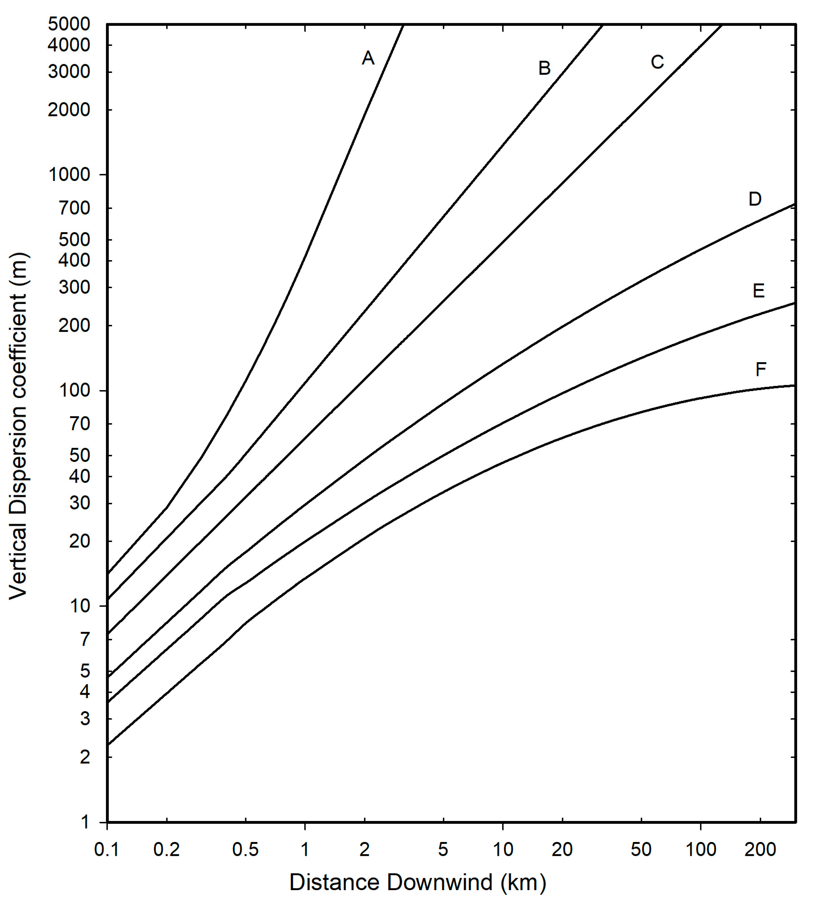
In Equations (8), (10), and (12), a key parameter is the value of H , and therefore x H , as discussed at length by Rowe et al. [14] in their Supplementary Materials. For strong winds, i.e., V > 6 m/s at 10 m height and at nighttime or low solar insolation, the atmosphere can be considered as neutral in the so-called Pasquill–Gifford–Turner classification [43,44,45], which means there is no tendency for enhancement of air turbulence (instability) or suppression (stability) through buoyancy effects. In fact, it is known that airborne pollutants emitted locally are transported and dispersed within the so-called atmospheric boundary layer (ABL: the tropospheric bottom layer), whose thickness is usually lower than one thousand meters [46], except for strongly unstable atmospheres. At any distance from the source, an order of magnitude value of H versus x can be estimated using the vertical dispersion length used for Gaussian plumes and shown in Figure 2 [47,48].
The wind itself depends on the altitude, but its variations above ten meters are rather small within the ABL [49]. In the next section, therefore, it will be assumed to be independent of altitude and taken as the ten-meter value.

3.3. Possible Airborne Epidemic Triggering via Long-Range Transmission

Let us now consider two highly populated areas, designated as the “source” and the “target”, respectively, separated by an unpopulated area (no man’s land). The source population is considered as infected whereas no sick people are initially present in the target area (hereafter box 3). At the downwind border of the source (hereafter box 1) characterized by a length L1, it is possible to quantify the quantum concentration n1,q(L1) following Equation (8) taking into account that at the upstream border of the source n1,q(x1 = 0) = 0. The downwind border of the source also coincides with the upwind border of the “no man’s land” section (hereafter box 2). However, as explained further in Section 4.2, the dispersive height H in box 2 (H2) is higher than in box 1 (H1). This impacts the initial quantum concentration n2,q(x2 = 0) by a factor of H1/H2 at the upstream border of box 2 such that:
n2,q(x2 = 0) = H1/H2 × n1,q(L1)
The evolution of the quantum concentration n2,q(x2) in box 2 is then governed only by the virus lifetime according to Equation (9) since D I = 0 in box 2. This leads to a new value n2,q(L2) at the downstream border L2 of box 2. Again, this border coincides with the upstream border of the target area, box 3. At this interface, however, the dispersive height is not modified compared to box 2 (H3 = H2) since H2 is already taken as an upper limit of the ABL thickness (see Section 4.2). The quantum concentration entering box 3 is then n3,q(x3 = 0) = n2,q(L2). The quantum concentration n3,q(x3) can be considered as spatially and temporally constant within box 3 provided that:
  • The pathogen lifetime is clearly larger than the hydrodynamic time within the target depth, which is typically around 10–20 km.
  • The width of the target is less than the width of the source.
  • The emission source rate and meteorology do not change significantly during the time of exposure.
From this, the calculation of a probability of infection P t in the target area of population N t (assumed healthy and therefore susceptible) can be obtained combining Equations (2) and (4).
It follows that the statistical number of contaminated susceptible people S c is:
S c = P t × N t = 1 exp n 2 , q L 2 × p × t × N t
As exemplified below in Section 4.2, the value of P t will most often be extremely small, which shows a quasi-zero risk at the individual level as already discussed by Rowe et al. [14]. However, when the target is composed of a very high number N t of individuals, then a few people (≥1) could be infected. Of course, this process alone cannot sustain an epidemic but creates a few infectors (“primary cases”) which may trigger it.
In the next section, we examine a hypothetical case study of the creation of COVID-19 primary cases in northern France from southern England in wintertime when the strongest winds are most often from west to east in Western Europe.

4. Results for a Hypothetical Case of Long-Range Transmission of COVID-19 from Southern England to Northern France

4.1. General Considerations

In the recent pandemic of COVID-19, although it was originally discredited by governments and even health agencies, it is now well accepted that COVID-19 is mainly transmitted via bio-aerosols ([11] and references therein). This has brought focus to the need for ventilation of interior spaces and the need for mask wearing, amongst general measures specific to this contamination route.
The first thing to remember is that the SARS-CoV-2 virus is, first and foremost, a nanoparticle (diameter on the order of 100 nm). It can be exhaled by an infected person (hereafter infector) when confined within microdroplets of micron and submicron size [7,8]. These microdroplets originate from respiratory fluids, which, besides water as the main component, include a variety of other minor components: proteins, salt, etc. [50]. Water can evaporate leading to the creation of “dry nuclei”, which include these minor components together with the virus. Due to the presence of non-volatile components, the reduction in size of the microdroplets cannot exceed a factor of around 0.4.
The fact that the exhaled viruses are embedded in microparticles means that they can float in the air for extended periods, driven by air currents such as with aerosols. Therefore, as discussed in Section 2, this aerosol can travel over distances well beyond one hundred kilometers. The key question as to whether it can remain infectious after such travel is discussed in Section 5 where it is shown that the answer is strongly dependent on the geography and seasonality.
Some time ago, saw the emergence of the more infectious Delta variant, apparently with an origin in India, and sometime later, the even more infectious Omicron strain first identified in South Africa but which quickly became rampant in the United Kingdom and worldwide. As discussed in another of our recent papers [6], the higher viral load or higher contagiousness of these new variants results in an even higher infection risk via the airborne route. Following various outbreaks, we saw borders closing to try to contain the epidemic but with little success.

4.2. Details of the Long-Range Model of Transmission for the Present Hypothetical Case

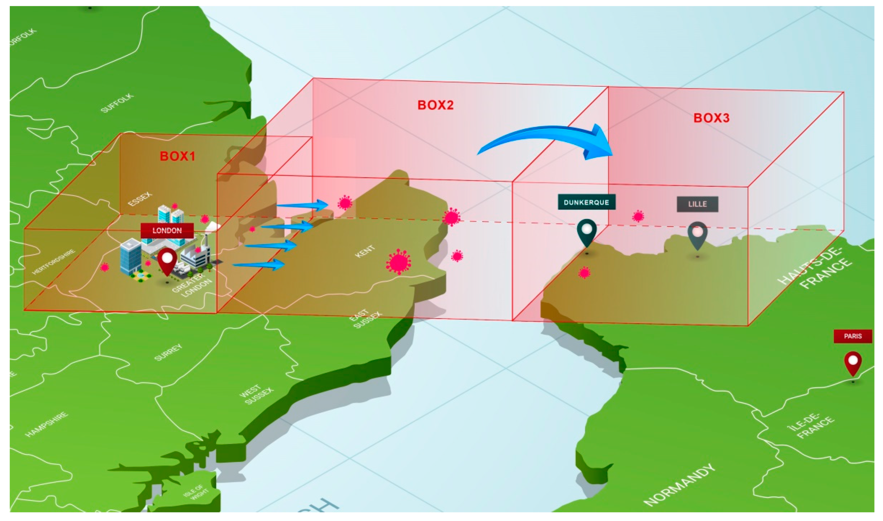
An infographic image of a model of three boxes is shown in Figure 3. Following the discussion in Section 3.3, we consider the first box in southern England corresponding to the upstream source of contamination. Roughly speaking, it corresponds to the greater London area and its downwind region. Although the county of Kent, to the southeast of London, is quite heavily populated, we shall restrict ourselves to a source around London with a width W of 40 km and a length L1 of 45 km, an area inside which we assume a population Np (x1 = 45 km) of 11 million people.
We can use the equations developed in Section 3.2 to make an estimate of the quantum concentration n1,q(L1) at the downwind border of this source box. However, the following problem arises: in wintertime, most of the quanta will be emitted indoors, with a room temperature around 20 °C and a rather low relative humidity (RH) (we assume 35% as a mean), but outdoors they are transported by the wind at low temperature (around 5 °C) and rather high humidity (80%) conditions, where the virus lifetime (see discussion in Section 5) is expected to be much longer than the atmospheric transport (hydrodynamic) time. Therefore, viral inactivation, as discussed in Section 5.2, will only occur indoors, via thermal effects at rather low RH. Indoor air is continuously renewed as contaminated air is evacuated outdoors with a characteristic time equal to 1 / A C H where A C H is the number of times that the total air volume in a room is completely removed and replaced in an hour. Therefore, the effect of viral inactivation indoors prior to evacuation can be taken as a reduction of the quantum emission rate per infector used in Section 3.2 following the formula:
q e f f = q × exp ( 1 / A C H × τ i
with the conservative hypothesis of A C H = 2   h 1 and τ i = 2   h (which is a good order of magnitude at 20 °C and low RH in indoor conditions at the source; see references in Section 5.2 as for instance [51]); this results in q e f f = 0.78 × q .
Once outdoors, the typical wintertime low temperatures and the absence of significant UV solar radiation [52,53] will ensure a very long virus lifetime as discussed in Section 5. Thus, the simple formula, Equation (12), can be used, with q e f f instead of q , to estimate the quantum concentration at the downwind border of the source. The dispersive height H 1 is estimated from Figure 2 as 300 m (for x1 = 45 km and state D in Figure 2), the population within the source is assumed as 1.1 × 10 7 , the wind velocity taken as 30 km/h, the width of the source as W = 40 km (which influences the density of infectors if Equation (10) is used in place of (12)), and the quantum production rate of an infector as 10 h−1. The numerical application leads to n 1 , q 45   km = 7.15 × 10 6   m 3 assuming a proportion of infected persons of r = 0.03 in the greater London area.
Turbulent mixing and transport by the wind will then lead quanta to the upstream border of the target area whose width is assumed less than or equal to the width of the source as stated in Section 3.3. Again, due to meteorological conditions (mean temperature around 5 °C, mean RH around 80% [54], and absence of UV radiation), the virus lifetime is much higher than the convective hydrodynamic time (which is <10 h, see following tables) for distances up to 250 km, and therefore the reduction in quantum concentration is solely due to the increase of the dispersive height H . Then, in such conditions n2,q(L2) = n2,q(x2 = 0). Using a conservative estimate for H   of 1000 m, a value corresponding to a common upper value of ABL thickness for neutral or stable conditions [46] results in a numerical value of n 3 , q x 3 = 0 of 2.15 × 10 6   m 3 at the upstream border of one of our targets.
We consider two plausible targets in France, either the city of Dunkerque or the Lille agglomeration, with populations of 0.2 × 10⁶ and 1.2 × 10⁶ people, respectively. We assume that the wind direction is the same as the direct path between the source and the target, a dominant direction in wintertime, which roughly corresponds to a wind direction from the west/northwest (respectively 288 and 294 degrees). As before, we also assume a wind velocity of 30 km/h, which is only slightly higher than the mean wind velocity in February/early March [55]. Note again that both target areas have a width across the wind less than that of the source. Table 1 gathers the main characteristics of the three boxes as depicted in Figure 3. Table 2 summarizes the assumed values of various parameters leading to a statistical number of primary cases. Since this number appears to be a few units in the frame of our assumptions, it clearly reveals the potential for an infection being triggered through long-range transportation of airborne viruses.
Note that the purpose of the calculations presented in Table 2 is solely to demonstrate the possible creation of a few primary cases. Changing the wind speed and other parameter values in a reasonable manner does not alter this conclusion. It could also be possible to refine the calculation considering a much longer time of exposure (several days) and the fact that virions in the target box can be inactivated indoors by thermal and RH effects such as those assumed for the source box, but again without changing the major conclusion.
From this table, it can be inferred that creation of only one primary case is possible within a day even with a much lower proportion of infectors such as for instance r~0.3%.

5. Discussion

5.1. Validity of the Atmospheric Box Model

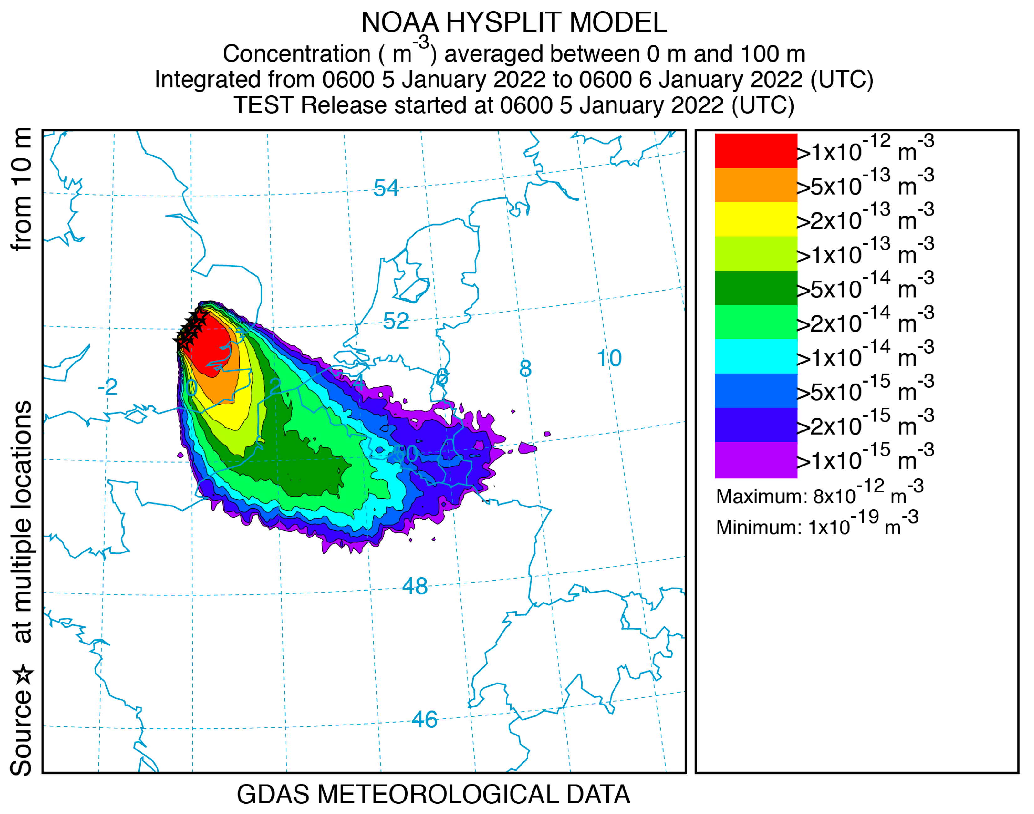
To determine if the box model assumptions were sufficiently realistic, a test calculation was performed using a three-dimensional particle transport and dispersion model. The HYSPLIT model [56] was selected for the simulation using one-degree resolution, gridded global meteorological data available at three-hour intervals from the National Oceanic and Atmospheric Administration (NOAA). As noted earlier, west-to-east flow is common, and a 24 h period (beginning 0600 UTC 5 January 2022) with airflow from London to France was identified in the first week of data downloaded from the GDAS server [57]. The model was configured to be similar to the box model. A 40 km line of five-point sources, orthogonal to the wind direction, was set over central London with a total emission rate of one unit per hour for the 24 h simulation period. Air concentrations (unit mass per volume) were computed as a 24 h average on a 10 km resolution grid with a vertical depth of 100 m to represent the surface layer for human exposure. Particles were terminated after 12 h to constrain the downwind domain to France rather than all of Western Europe. The HYSPLIT result depicted in Figure 4 shows a broad region of concentrations of around 5 × 10⁻¹⁴ m−3 over northeastern France. Using the effective quantum production rate qeff value derived from Table 2, the unit emission HYSPLIT values (through the expression: NP × r × qeff × 24) yield a quantum concentration of 3.1 × 10⁻⁶ quantum m−3, which is very close to the upstream box model value of 2.1 × 10⁻⁶. Due to the line source configuration, lateral dispersion along the centerline would be negligible, and the concentration results would primarily depend upon the vertical mixing. An examination of the diagnostic vertical mass profile after 12 h (not shown) indicates that 94% of the mass was in the first 1200 m above ground and 99% was within the first 1500 m, consistent with the well-mixed box model assumptions.
HYSPLIT is a much more refined model than the simple box model, which has for sole merit its simplicity, which allows us to rapidly derive an order of magnitude and to discuss the importance of various parameters.

5.2. The Question of the Virus Lifetime Indoor and Outdoor in Bio-Aerosol Form

The virus lifetime used in the above atmospheric model is defined, as stated above, using the analog in time of Equation (9):
n q t = n q 0 × exp ( t τ i )
As shown in the previous sections, the effect of virus lifetime is critical for the possibility of virus transmission over long distances, with a transport (hydrodynamic) time τ h as defined in Section 3.2. If, for τ i τ h , the decrease in quantum concentration downstream of a laterally extended source is mainly due to vertical atmospheric dispersion, for τ i τ h the quantum concentration will drop to an even much lower value, with a ratio of τ i / τ h . This condition corresponds to a distance to the source x   τ i × V where the transmission probability drops essentially to zero.
A lifetime on the same order of magnitude as the hydrodynamic time τ i ~ τ h will result in a reduction of active viruses (i.e., of quantum concentration) in the area where they could infect susceptible people, but this will not change the conclusions in Section 4.2: the number of primary cases due to long-distance infection will remain higher than unity.
Indoors, viruses are inactivated by a variety of factors, but it is recognized that the principal ones are temperature and humidity. The effect of humidity on lifetime is rather difficult to assess [58,59]. After some discussion [60] about whether to consider absolute humidity (AH) or relative humidity (RH), it has been concluded that RH drives the virus lifetime with a U-shaped curve for τ i = f R H . This behavior is due to the variation of the solute/solvent concentrations in the aqueous solution of the infectious microdroplet. This U-shape has been rationalized by Morris et al. [61] considering the efflorescence relative humidity (ERH), which corresponds to the RH below in which a spontaneous evaporation of a salty water solution initiates a crystallization called efflorescence (leading then to what is called dry nuclei for viral bio-aerosols). Note that the inverse process, when RH is increased, is called deliquescence [62].
The inverse of the lifetime k can be considered as a rate of inactivation (unit = time−1), and it is generally admitted [61,63] that, for a given value of RH, it follows an Arrhenius law with temperature:
k = A × exp E a R × T
On the basis of numerous experimental results for a variety of viruses, this behavior has been rationalized by Yap et al. [63] as viral protein denaturation via thermal effects, including for SARS-CoV-2. In this latter case, Yap et al. report values of E a = 135.69 kJ/mole and A = 1.3 × 10²¹ min−1, respectively.
There are clearly large uncertainties in the exact lifetime of SARS-CoV-2 in aerosol form at given values of RH and temperature. For example, van Doremalen et al. [51] report a value of 1–3 h at a temperature of 21–23 °C and RH of 40% although Fears et al. [64] found a much higher value (up to sixteen hours). On the other hand, a group from Bristol (UK) has recently reported a very fast loss of infectivity (seconds to minutes) of virions aerosolized from a tissue culture medium, hereafter TCM, at room temperature [65]. Note, however, that Oswin et al. do not observe an exponential decay but instead a plateau after an initial rapid loss, preventing the determination of a virus lifetime as defined using Equation (16). Note also that Smither et al. [66] have reported very different losses of infectivity between bio-aerosols generated from TCM and artificial saliva and that, in real life, respiratory fluids should be used. A short (few minutes) lifetime in aerosols for normal indoor conditions would not be compatible with airborne transmission, which however, has been widely confirmed and documented [11].
The large uncertainty in lifetime can be understood due to the extreme difficulty of virus concentration measurements in air and, worse, of their characterization as to whether they are active or not [20].
In any case, based on most of the above studies and others [20,51,61,63], the order of magnitude of the virus lifetime as defined by Equation (16) is around one to a few hours at room temperature, a magnitude that we have taken into account in the estimation of the reduction of quantum production at the source in Section 4.2 (Equation (15)).
Outdoors, considering temperature and humidity, it can then easily be shown that at low temperatures (<5 °C) and large RH (around 80%), SARS-CoV-2 has a lifetime of at least several tens of hours, an important conclusion, which has been used in our box model. However, solar UV radiation is very efficient for virus inactivation [52], but this effect has not been considered since we are restricting ourselves to the case of mean and high latitudes in winter, where nighttime is much longer than daytime, and where the sky is often overcast during the day, making UV inactivation negligible outdoors during atmospheric virus transport. In fact, this conclusion holds even for a clear sky, at least from early November to the end of February, at a latitude around 51° N due to the large solar zenith angle, which then reduces the efficiency of UV virus inactivation by orders of magnitude, due to ozone absorption of solar UV [52]. In fact, calculations leading exactly to the same conclusion have been developed in a recent paper of Sagripanti and Lytle [53].
A much more elusive and not clearly recognized effect outdoors is the so-called open air factor (hereafter OAF). Experiments were conducted in the late nineteen sixties and early seventies by a few researchers on the survival of some pathogens indoors and outdoors. May and Druett [67,68] conducted experiments on Escherichia Coli deposited on ultrafine spider thread and observed a much shorter survival time outdoors than indoors. They named this effect open air factor. As some of the experiments were conducted at night, they invoked the possibility that some chemical due to pollution could be present outdoors. Donaldson and Ferris [69] have conducted the same kind of experiments both with the foot and mouth disease pathogens and Escherichia Coli, but reported experiments in the literature remain extremely sparse. This effect has also been studied in the frame of biological weapons, but most of the results were classified [70].
The recent COVID-19 pandemic has reactivated the interest in OAF, and a few papers have appeared on this question [71,72]. There are no laboratory results, and they do not offer any further evidence beyond the very few results reported around fifty years ago. One of the arguments in favor of the OAF, found in the literature [73], is that high indoor ventilation using fresh outdoor air considerably reduces the risk of infection, but this is clearly understood in the framework of the Wells–Riley model and its avatars [14,16,74].
Due to the scarcity of laboratory work, the idea cannot be excluded that some artefacts could have been introduced in the seminal results of May and Druett. More experiments conducted with modern means are necessary to say whether or not OAF should be taken into account. Let us note than in chapter 3.2.8 entitled “Aerobiology of Agricultural Pathogens” of Manual of Environmental Microbiology [75], OAF is not even mentioned; neither is it mentioned in a recent review paper about “current understanding of airborne transmission of important viral animal pathogens in spreading disease” [33]. Therefore, although this effect cannot be totally excluded, on the basis of the present knowledge of the SARS-CoV2 virus, it cannot be taken into account quantitatively in any outdoor model of COVID-19 transmission.

5.3. The Very Low Dose Question

That a single susceptible person inhales numerous virions transported by the wind over long distances is of course highly unlikely. Therefore, in the framework of the present paper, the question of the dose/risk function at very low dose deserves a careful discussion.
The literature on virus transmission very often refers to a quantity named “Minimum Infective Dose” with the acronym MID. As stated by Haas et al. [20], however, the term “minimum” is very misleading since it seems to imply a minimum number of pathogens needed to trigger an infection and should be replaced by “median”. A real minimum would imply a thresholding effect, which is not observed experimentally. If such an effect existed, it would prevent the long-distance transmission presented above. However, there exists a large quantity of literature on the subject of the dose/risk link [19,20,21,22], and most authors conclude that a single pathogen can trigger infection [19], although with a small probability (single-hit models). The exponential dose–risk function used in the present paper is clearly without a threshold and is used widely elsewhere. Together with the quantum concept, it completely takes care of the statistical and probabilistic aspects of the transmission problem. As a quantum corresponds to hundreds of viruses, the idea that is sometimes reported that it is necessary to inhale at least a quantum to be contaminated is completely wrong.

6. Conclusions

In the present paper, we have shown, with a rather simple model of conservation equations and a dose–risk function, that creation of primary cases at large distances from a densely populated and infected area is possible if the target is itself a large population. Surprisingly, this is well known and accepted in veterinary science, but the link with human airborne transmission, to our knowledge, has not been made. Our simple atmospheric “box” model has been validated in a specific case using a three-dimensional dispersion (HYSPLIT) calculation, using actual meteorological data.
In order to derive orders of magnitude, we have chosen to use simple existing models that have been adapted to the described problem, although it is clear that it is very complex by nature. For example, we have not taken into account the variety within populations of either infectors or susceptible people, such as gender or age. Similarly, we have not considered the level and nature of activities that at an individual level influence the production rate of bio-aerosols. Nevertheless, since our modeling deals with large numbers in terms of source and target populations, these omissions are sensible. However, the only hypotheses that could completely hinder our conclusions would be that: first the airborne transmission route is negligible compared to other modes of infection or secondly that the lifetime of the virus embedded in the bioaerosol is very short in any physical conditions. These two hypotheses are in our opinion not supported by the thorough analysis of the literature presented above.
Note also, the conclusions of the recent paper are restricted to meteorological conditions where the atmosphere can be considered neutral or stable (cases D–F in Figure 2). Therefore, they do not apply to an unstable atmospheric state, which can be found for example on a sunny day with moderate wind [48].
One of the consequences of the present investigation is that the hunt for “patient zero” can sometimes be meaningless. It also shows that, on the level of a continent, viruses ignore borders, and infection can spread downwind of a contaminated region irrespective of the cross-border movement of persons. However, due to the importance of climate on the virus lifetime and atmospheric state, it must be kept in mind that the conclusions and hypotheses presented here apply mainly to mid and high latitudes under winter conditions.
Although it has not been discussed in the present paper, it should be noted that in February 2021, most of the contamination in Dunkerque by COVID-19 was due to the British variant [76], which could have started via the process described above. It would of course be extremely interesting to conduct a more refined analysis than that presented here concerning a longer period and using available epidemiological and atmospheric data. The purpose of the present study is only to highlight the possibility of the process.
Finally, all the measures that have been taken to avoid the transfer of the COVID-19 pandemic from one region or country to another have shown to be mostly ineffective. The main objective of the present paper is to show that governments and health agencies should concentrate on mitigation measures that avoid disease spread rather than simply on the deterrence of international or regional transmission. We are not immune to a potential new respiratory disease that could be worse than COVID-19, with, for example, numerous lethal cases in the young population. The prevention of the spread of such a future disease must be prepared for by considering the biological aspect of indoor air quality, through new norms of ventilation and air treatment as discussed in [6].

Author Contributions

B.R.R.: Conceptualization; Methodology; Investigation; Validation; Writing—original draft; Writing—review and editing. J.B.A.M.: Writing—original draft; Writing—review and editing. A.C.: Validation; Writing—review and editing. R.D.: HYSPLIT validation of the simple box model; Writing—review and editing. All authors have read and agreed to the published version of the manuscript.

Funding

The authors declare that no funds, grants, or other support were received during the preparation of this manuscript.

Institutional Review Board Statement

Not applicable.

Informed Consent Statement

Not applicable.

Data Availability Statement

All data generated or analyzed during this study are included in this published article.

Acknowledgments

Bertrand Rowe wishes to thank Daniel Preston of Rice University and Lidia Morawska of Queensland University of Technology for very helpful discussions on SARS-CoV-2 virus lifetimes, as well as Melinda Rowe for her help as digital designer.

Conflicts of Interest

The authors declare no conflict of interest.

References

  1. Giesecke, J. Primary and index cases. Lancet 2014, 384, 2024. [Google Scholar] [CrossRef] [PubMed]
  2. MaGee, J.; Arora, V.; Ventresca, M. Identifying the source of an epidemic using particle swarm optimization. In Proceedings of the 2022 Genetic and Evolutionary Computation Conference (Gecco’22), Boston, MA, USA, 9–13 July 2022; pp. 1237–1244. [Google Scholar]
  3. Snow, J. On the Mode of Communication of Cholera, 2nd ed.; John Churchill: London, UK, 1855. [Google Scholar]
  4. Carinci, F. COVID-19: Preparedness, decentralisation, and the hunt for patient zero Lessons from the Italian outbreak. Br. Med. J. 2020, 368, 1–2. [Google Scholar]
  5. Lu, D. The hunt to find the coronavirus pandemic’s patient zero. New Sci. 2020, 245, 9. [Google Scholar] [CrossRef] [PubMed]
  6. Rowe, B.R.; Canosa, A.; Meslem, A.; Rowe, F. Increased airborne transmission of COVID-19 with new variants, Implications for health policies. Build. Environ. 2022, 219, 109132. [Google Scholar] [CrossRef] [PubMed]
  7. Tang, J.W.; Bahnfleth, W.P.; Bluyssen, P.M.; Buonanno, G.; Jimenez, J.L.; Kurnitski, J.; Li, Y.; Miller, S.; Sekhar, C.; Morawska, L.; et al. Dismantling myths on the airborne transmission of severe acute respiratory syndrome coronavirus-2 (SARS-CoV-2). J. Hosp. Infect. 2021, 110, 89–96. [Google Scholar] [CrossRef]
  8. Greenhalgh, T.; Jimenez, J.L.; Prather, K.A.; Tufekci, Z.; Fisman, D.; Schooley, R. Ten scientific reasons in support of airborne transmission of SARS-CoV-2. Lancet 2021, 397, 1603–1605. [Google Scholar] [CrossRef]
  9. Morawska, L.; Tang, J.L.W.; Bahnfleth, W.; Bluyssen, P.M.; Boerstra, A.; Buonanno, G.; Cao, J.J.; Dancer, S.; Floto, A.; Franchimon, F.; et al. How can airborne transmission of COVID-19 indoors be minimised? Environ. Int. 2020, 142, 105832. [Google Scholar] [CrossRef]
  10. Randall, K.; Ewing, E.; Marr, L.; Jimenez, J.L.; Bourouiba, L. How did we get here: What are droplets and aerosols and how far do they go? A historical perspective on the transmission of respiratory infectious diseases. Interf. Foc. 2021, 11, 20210049. [Google Scholar] [CrossRef]
  11. Wang, C.C.; Prather, K.A.; Sznitman, J.; Jimenez, J.L.; Lakdawala, S.S.; Tufekci, Z.; Marr, L.C. Airborne transmission of respiratory viruses. Science 2021, 373, eabd9149. [Google Scholar] [CrossRef]
  12. Morawska, L.; Cao, J. Airborne Transmission of SARS-CoV-2: The World Should Face the Reality. Environ. Int. 2020, 139, 105730. [Google Scholar] [CrossRef]
  13. New York Times 239 Experts with One Big Claim the Coronavirus is Airborne. 2021. Available online: https://www.nytimes.com/2020/07/04/health/239-experts-with-one-big-claim-the-coronavirus-is-airborne.html (accessed on 1 June 2021).
  14. Rowe, B.R.; Canosa, A.; Drouffe, J.M.; Mitchell, J.B.A. Simple quantitative assessment of the outdoor versus indoor airborne transmission of viruses and COVID-19. Environ. Res. 2021, 198, 111189. [Google Scholar] [CrossRef]
  15. Wells, W.F. Airborne Contagion and Air Hygiene. An Ecological Study of Droplet Infections; Harvard University Press: Cambridge, MA, USA, 1955. [Google Scholar]
  16. Riley, E.C.; Murphy, G.; Riley, R.L. Airborne Spread of Measles in A Suburban Elementary-School. Am. J. Epidemiol. 1978, 107, 421–432. [Google Scholar] [CrossRef]
  17. Ortolano, L. Estimating Air Quality Impacts. Environ. Impact. Assess. Rev. 1985, 5, 9–35. [Google Scholar] [CrossRef]
  18. Khan, S.; Hassan, Q. Review of developments in air quality modelling and air quality dispersion models. J. Environ. Eng. Sci. 2021, 16, 1–10. [Google Scholar] [CrossRef]
  19. Brouwer, A.F.; Weir, M.H.; Eisenberg, M.C.; Meza, R.; Eisenberg, J.N.S. Dose-response relationships for environmentally mediated infectious disease transmission models. PLoS Comput. Biol. 2017, 13, e1005481. [Google Scholar] [CrossRef] [Green Version]
  20. Haas, C.N.; Rose, J.B.; Gerba, C.P. Quantitative Microbial Risk Assessment; John Wiley & Sons, Inc.: Hoboken, NJ, USA, 2014. [Google Scholar]
  21. Teunis, P.F.M.; Havelaar, A.H. The Beta Poisson dose-response model is not a single-hit model. Risk Anal. 2000, 20, 513–520. [Google Scholar] [CrossRef] [PubMed]
  22. Zwart, M.P.; Hemerik, L.; Cory, J.S.; de Visser, J.; Bianchi, F.J.; Van Oers, M.M.; Vlak, J.M.; Hoekstra, R.F.; Van der Werf, W. An experimental test of the independent action hypothesis in virus-insect pathosystems. Proc. R. Soc. B Biol. Sci. 2009, 276, 2233–2242. [Google Scholar] [CrossRef] [Green Version]
  23. Fuchs, N.A. The Mechanics of Aerosols; Dover Publication: Mineola, NY, USA, 1989. [Google Scholar]
  24. Francis, D.; Fonseca, R.; Nelli, N.; Bozkurt, D.; Picard, G.; Guan, B. Atmospheric rivers drive exceptional Saharan dust transport towards Europe. Atmos. Res. 2022, 266, 105959. [Google Scholar] [CrossRef]
  25. Allen, S.; Allen, D.; Baladima, F.; Phoenix, V.R.; Thomas, J.L.; Le Roux, G.; Sonke, J.E. Evidence of free tropospheric and long-range transport of microplastic at Pic du Midi Observatory. Nat. Com. 2021, 12, 7242. [Google Scholar] [CrossRef]
  26. Martins, L.D.; Hallak, R.; Alves, R.C.; de Almeida, D.S.; Squizzato, R.; Moreira, C.A.B.; Beal, A.; da Silva, I.; Rudke, A.; Martins, J.A. Long-range Transport of Aerosols from Biomass Burning over Southeastern South America and their Implications on Air Quality. Aerosol Air Qual. Res. 2018, 18, 1734–1745. [Google Scholar] [CrossRef] [Green Version]
  27. Rousseau, D.D.; Duzer, D.; Cambon, G.V.; Jolly, D.; Poulsen, U.; Ferrier, J.; Schevin, P.; Gros, R. Long distance transport of pollen to Greenland. Geophys. Res. Lett. 2003, 30, 1765. [Google Scholar] [CrossRef]
  28. Dillon, C.F.; Dillon, M.B. Multiscale Airborne Infectious Disease Transmission. Appl. Environ. Microbiol. 2021, 87, e02314-20. [Google Scholar] [CrossRef] [PubMed]
  29. Donaldson, A.I.; Gloster, J.; Harvey, L.D.J.; Deans, D.H. Use of prediction models to forecast and analyse airborne spread during the foot-and-mouth disease outbreaks in Brittany, Jersey and the Isle of Wight in 1981. Veter. Rec. 1982, 110, 53–57. [Google Scholar] [CrossRef]
  30. Garner, M.; Hess, G.; Yang, X. An integrated modelling approach to assess the risk of wind-borne spread of foot-and-mouth disease virus from infected premises. Environ. Mod. Assess. 2006, 11, 195–207. [Google Scholar] [CrossRef]
  31. Gloster, J.; Sellers, R.F.; Donaldson, A.I. Long distance transport of foot-and-mouth disease virus over the sea. Veter. Rec. 1982, 110, 47–52. [Google Scholar] [CrossRef]
  32. Hagerman, A.D.; South, D.D.; Sondgerath, T.C.; Patyk, K.A.; Sanson, R.L.; Schumacher, R.S.; Delgado, A.H.; Magzamen, S. Temporal and geographic distribution of weather conditions favorable to airborne spread of foot-and-mouth disease in the coterminous United States. Prev. Veter. Med. 2018, 161, 41–49. [Google Scholar] [CrossRef]
  33. La, A.; Zhang, Q.; Cicek, N.; Coombs, K.M. Current understanding of the airborne transmission of important viral animal pathogens in spreading disease. Biosyst. Eng. 2022, 224, 92–117. [Google Scholar] [CrossRef]
  34. Lambkin, K.; Hamilton, J.; McGrath, G.; Dando, P.; Draxler, R. Foot and Mouth Disease atmospheric dispersion system. Adv. Sci. Res. 2019, 16, 113–117. [Google Scholar] [CrossRef] [Green Version]
  35. Gloster, J.; Jones, A.; Redington, A.; Burgin, L.; Sorensen, J.H.; Turner, R.; Dillon, M.; Hullinger, P.; Simpson, M.; Astrup, P.; et al. Airborne spread of foot-and-mouth disease-Model intercomparison. Veter. J. 2010, 183, 278–286. [Google Scholar] [CrossRef] [Green Version]
  36. Coffman, M.S.; Sanderson, M.; Dodd, C.C.; Arzt, J.; Renter, D.G. Estimation of foot-and-mouth disease windborne transmission risk from USA beef feedlots. Prev. Veter. Med. 2021, 195, 105453. [Google Scholar] [CrossRef] [PubMed]
  37. Zhao, Y.; Richardson, B.; Takle, E.; Chai, L.L.; Schmitt, D.; Xin, H.W. Airborne transmission may have played a role in the spread of 2015 highly pathogenic avian influenza outbreaks in the United States. Sci. Rep. 2019, 9, 11755. [Google Scholar] [CrossRef] [PubMed] [Green Version]
  38. Cannon, R.M.; Garner, M.G. Assessing the risk of wind-borne spread of foot-and-mouth disease in Australia. Environ. Int. 1999, 25, 713–723. [Google Scholar] [CrossRef]
  39. Sutmoller, P.; Vose, D.J. Contamination of animal products: The minimum pathogen dose required to initiate infection. Rev. Sci. Tech. Off. Int. Epizoot. 1997, 16, 30–32. [Google Scholar] [CrossRef]
  40. Mareddy, A.R. Impacts on air environment. In Environmental Impact Assessment: Theory and Practice; Elsevier, Inc.: Amsterdam, The Netherlands, 2017; pp. 171–216. [Google Scholar]
  41. Canter, L.W. Air Quality Impacts. In Environmental Impacts of Agricultural Production Activities; CRC Press: Boca Raton, FL, USA, 1986; pp. 169–224. [Google Scholar]
  42. Nelson, K.E.; LaBelle, S.J. Handbook for the Review of Airport Environmental Impact Statements; ANL/ES-46; Argonne National Laboratory: Argonne, IL, USA, 1975. [Google Scholar]
  43. Gifford, F.A. Use of Routine Meteorological Observations for Estimating Atmospheric Dispersion. Nucl. Saf. 1961, 2, 47–51. [Google Scholar]
  44. Pasquill, F. The estimation of the dispersion of windborn material. Meteorol. Mag. 1961, 90, 33–49. [Google Scholar]
  45. Turner, D.B. Workbook of Atmospheric Dispersion Estimates: An Introduction to Dispersion Modeling, 2nd ed.; CRC Press, Lewis Publishers: Boca Raton, FL, USA, 1994. [Google Scholar]
  46. Sáez de Cámara Oleaga, E. Air Pollution and Its Control Technologies. 2016. Available online: https://ocw.ehu.eus/course/view.php?id=389 (accessed on 12 January 2022).
  47. Seinfeld, J.H.; Pandis, S.N. Atmospheric Chemistry and Physics: From Air Pollution to Climate Change, 3rd ed.; John Wiley & Sons, Inc.: Hoboken, NJ, USA, 2016. [Google Scholar]
  48. Turner, D.B. Workbook of Atmospheric Dispersion Estimates; U.S. Environmental Protection Agency, Office of Air Programs: Chapel Hill, NC, USA, 1970; Volume AP-26. [Google Scholar]
  49. Hsu, S.A.; Meindl, E.A.; Gilhousen, D.B. Determining the Power-Law Wind-Profile Exponent Under Near-Neutral Stability Conditions at Sea. J. Appl. Meteorol. 1994, 33, 757–765. [Google Scholar] [CrossRef]
  50. Nicas, M.; Nazaroff, W.W.; Hubbard, A. Toward understanding the risk of secondary airborne infection: Emission of respirable pathogens. J. Occup. Environ. Hyg. 2005, 2, 143–154. [Google Scholar] [CrossRef]
  51. van Doremalen, N.; Bushmaker, T.; Morris, D.H.; Holbrook, M.G.; Gamble, A.; Williamson, B.N.; Tamin, A.; Harcourt, J.L.; Thornburg, N.J.; Gerber, S.I.; et al. Aerosol and Surface Stability of SARS-CoV-2 as Compared with SARS-CoV-1. N. Eng. J. Med. 2020, 382, 1564–1567. [Google Scholar] [CrossRef]
  52. Lytle, C.D.; Sagripanti, J.L. Predicted inactivation of viruses of relevance to biodefense by solar radiation. J. Virol. 2005, 79, 14244–14252. [Google Scholar] [CrossRef] [Green Version]
  53. Sagripanti, J.L.; Lytle, C. Estimated Inactivation of Coronaviruses by Solar Radiation With Special Reference to COVID-19. Photochem. Photobiol. 2020, 96, 731–737. [Google Scholar] [CrossRef]
  54. Weather and Climate Average Humidity in London. 2022. Available online: https://weather-and-climate.com/average-monthly-Humidity-perc,London,United-Kingdom (accessed on 1 March 2022).
  55. Weather Sparks Weather in London. 2022. Available online: https://weatherspark.com/d/45062/2/11/Average-Weather-on-February-11-in-London-United-Kingdom#Figures-WindDirection (accessed on 1 March 2022).
  56. Stein, A.F.; Draxler, R.R.; Rolph, G.D.; Stunder, B.J.B.; Cohen, M.D.; Ngan, F. NOAA’s HYSPLIT Atmospheric Transport and Dispersion Modeling System. Bull. Am. Meteor. Soc. 2015, 96, 2059–2077. [Google Scholar] [CrossRef]
  57. National Centers for Environmental Information Global Data Assimilation System (GDAS). 2022. Available online: https://www.ncei.noaa.gov/access/metadata/landing-page/bin/iso?id=gov.noaa.ncdc:C00379 (accessed on 3 March 2022).
  58. Ijaz, M.K.; Brunner, A.H.; Sattar, S.A.; Nair, R.C.; Johnsonlussenburg, C.M. Survival Characteristics of Airborne Human Coronavirus-229E. J. Gen. Virol. 1985, 66, 2743–2748. [Google Scholar] [CrossRef] [PubMed]
  59. Yang, W.; Marr, L.C. Mechanisms by Which Ambient Humidity May Affect Viruses in Aerosols. Appl. Envir. Microbiol. 2012, 78, 6781–6788. [Google Scholar] [CrossRef] [PubMed] [Green Version]
  60. Marr, L.C.; Tang, J.W.; Van Mullekom, J.; Lakdawala, S.S. Mechanistic insights into the effect of humidity on airborne influenza virus survival, transmission and incidence. J. R. Soc. Interf. 2019, 16, 20180298. [Google Scholar] [CrossRef]
  61. Morris, D.H.; Yinda, K.C.; Gamble, A.; Rossine, F.W.; Huang, Q.S.; Bushmaker, T.; Fischer, R.J.; Matson, M.J.; Van Doremalen, N.; Vikesland, P.J.; et al. Mechanistic theory predicts the effects of temperature and humidity on inactivation of SARS-CoV-2 and other enveloped viruses. eLife 2021, 10, e65902. [Google Scholar] [CrossRef]
  62. Horst, D.; Zhang, Q.; Schmidt, E. Deliquescence and Efflorescence of Hygroscopic Salt Particles in Dust Cakes on Surface Filters. Chem. Eng. Technol. 2019, 42, 2348–2357. [Google Scholar] [CrossRef]
  63. Yap, T.F.; Liu, Z.; Shveda, R.A.; Preston, D.J. A predictive model of the temperature-dependent inactivation of coronaviruses. Appl. Phys. Lett. 2020, 117, 060601. [Google Scholar] [CrossRef]
  64. Fears, A.C.; Klimstra, W.B.; Duprex, P.; Hartman, A.; Weaver, S.C.; Plante, K.S.; Mirchandani, D.; Plante, J.A.; Aguilar, P.V.; Fernandez, D.; et al. Persistence of Severe Acute Respiratory Syndrome Coronavirus 2 in Aerosol Suspensions. Emerg. Infect. Dis. 2020, 26, 2168–2171. [Google Scholar] [CrossRef]
  65. Oswin, H.P.; Haddrell, A.E.; Otero-Fernandez, M.; Mann, J.F.S.; Cogan, T.A.; Hilditch, T.G.; Tiana, J.; Hardya, D.A.; Hill, D.J.; Finn, A.; et al. The dynamics of SARS-CoV-2 infectivity with changes in aerosol microenvironment. Proc. Natl. Acad. Sci. USA 2022, 119, e2200109119. [Google Scholar] [CrossRef]
  66. Smither, S.J.; Eastaugh, L.S.; Findlay, J.S.; Lever, M.S. Experimental aerosol survival of SARS-CoV-2 in artificial saliva and tissue culture media at medium and high humidity. Emerg. Microb. Infect. 2020, 9, 1415–1417. [Google Scholar] [CrossRef]
  67. Druett, H.A.; May, K.R. Unstable Germicidal Pollutant in Rural Air. Nature 1968, 220, 395–396. [Google Scholar] [CrossRef]
  68. May, K.R.; Druett, H.A. A Microthread Technique for Studying Viability of Microbes in a Simulated Airborne State. J. Gen. Microbiol. 1968, 51, 353–366. [Google Scholar] [CrossRef] [Green Version]
  69. Donaldson, A.I.; Ferris, N.P. The Survival of Foot-and-Mouth-Disease Virus in Open Air Conditions. J. Hyg. 1975, 74, 409–416. [Google Scholar] [CrossRef] [Green Version]
  70. Hood, A. The effect of open-air factors on the virulence and viability of airborne Francisella tularensis. Epidemiol. Infect. 2009, 137, 753–761. [Google Scholar] [CrossRef] [Green Version]
  71. Cox, R.; Ammann, M.; Crowley, J.N.; Griffiths, P.T.; Herrmann, H.; Hoffmann, E.H.; Jenkin, M.E.; McNeill, V.; Mellouki, A.; Penkett, C.J.; et al. Opinion: The germicidal effect of ambient air (open-air factor) revisited. Atmos. Chem. Phys. 2021, 21, 13011–13018. [Google Scholar] [CrossRef]
  72. Hobday, R.; Collignon, P. An Old Defence Against New Infections: The Open-Air Factor and COVID-19. Cureus J. Med. Sci. 2022, 14, e26133. [Google Scholar] [CrossRef] [PubMed]
  73. Hobday, R. The open-air factor and infection control. J. Hosp. Infect. 2019, 103, E23–E24. [Google Scholar] [CrossRef] [PubMed]
  74. Buonanno, G.; Morawska, L.; Stabile, L. Quantitative assessment of the risk of airborne transmission of SARS-CoV-2 infection: Prospective and retrospective applications. Environ. Int. 2020, 145, 106112. [Google Scholar] [CrossRef] [PubMed]
  75. Levetin, E. Aerobiology of Agricultural Pathogens. In Manual of Environmental Microbiology; Yates, M.V., Nakatsu, C.H., Miller, R.V., Pillai, S.D., Eds.; Wiley Online Library: Hoboken, NJ, USA, 2015; pp. 1–20. [Google Scholar]
  76. France Info COVID-19: Le Variant Anglais Détecté dans 68% des Tests Positifs à Dunkerque. 2021. Available online: https://www.francetvinfo.fr/sante/maladie/coronavirus/COVID-19-le-variant-anglais-detecte-dans-68-des-tests-positifs-a-dunkerque_4293213.html (accessed on 15 February 2021).
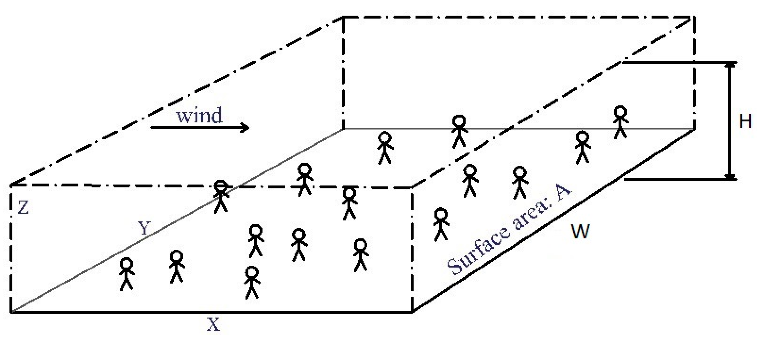
Figure 1. The atmospheric box model.
Atmosphere 14 01050 g001
Figure 2. Vertical dispersion length for Gaussian plumes. Classification of atmosphere state: A: Extremely unstable; B: Moderately unstable; C: slightly unstable; D: neutral; E: slightly stable; F: moderately stable.
Atmosphere 14 01050 g002
Figure 3. Model of three boxes between greater London and northern France. Note that the upstream border of box 3 is dependent on the considered target (i.e., either Dunkerque or Lille).
Atmosphere 14 01050 g003
Figure 4. Results of the HYSPLIT model.
Atmosphere 14 01050 g004
Table 1. Main characteristics of the three boxes used in the present model.
Box 1Box 2Box 3
Length: L (km)45150/230 a--- b
Width: W (km)4040<40
Dispersive height: H (m)30010001000
Wind speed V (km/h) 303030
nq (quanta/m3)7.1 × 10−6 c2.1 × 10−62.1 × 10⁻⁶
a: Depending on the considered target, either Dunkerque or Lille. b: This length is not fixed since it is not useful for the present estimation. c: Value at the downstream end of the box.
Table 2. Possible number of primary cases created (per day) via the long-distance transport of aerosols. London area population of 11 million; wind velocity: 30 km/h; exposure of 24 h; proportion of possible infectors in greater London: r = 3%; quantum production rate q = 10 h−1/infector.
DunkerqueLille
Distance from London, center to center (km)180244
Population (106)0.21.2
Hydrodynamic time (h)5.07.7
Upstream quantum concentration (m−3)2.1 × 10−62.1 × 10−6
Dose for 24 h2.6 × 10−52.6 × 10⁻⁵
Probability of infection Pt2.6 × 10−52.6 × 10⁻⁵
Number of primary cases531
Disclaimer/Publisher’s Note: The statements, opinions and data contained in all publications are solely those of the individual author(s) and contributor(s) and not of MDPI and/or the editor(s). MDPI and/or the editor(s) disclaim responsibility for any injury to people or property resulting from any ideas, methods, instructions or products referred to in the content.