Statistical PM_2.5 Prediction in an Urban Area Using Vertical Meteorological Factors

Abstract

A key concern related to particulate air pollution is the development of an early warning system that can predict local PM_2.5 levels and excessive PM_2.5 concentration episodes using vertical meteorological factors. Machine learning (ML) algorithms, particularly those with recognition tasks, show great potential for this purpose. The objective of this study was to compare the performance of multiple linear regression (MLR) and multilayer perceptron (MLP) in predicting PM_2.5 levels. The software was trained to predict PM_2.5 levels up to 7 days in advance using data from long-term measurements of vertical meteorological factors taken at five heights above ground level (AGL)—10, 30, 50, 75, and 110 m—and PM_2.5 concentrations measured 30 m AGL. The data used were collected between 2015 and 2020 at the Microclimate and Air Pollutants Monitoring Tower station at Kasetsart University, Bangkok, Thailand. The results showed that the correlation coefficients of PM_2.5 predicted and observed using MLR and MLP were in the range of 0.69–0.86 and 0.64–0.82, respectively, for 1–3 days ahead. Both models showed satisfactory agreement with the measured data, and MLR performed better than MLP at PM_2.5 prediction. In conclusion, this study demonstrates that the proposed approach can be used as a component of an early warning system in cities, contributing to sustainable air quality management in urban areas.

1. Introduction

Global research has focused on the air pollution parameter called PM_2.5, which refers to fine particulate matter with an aerodynamic diameter of less than 2.5 mm. In 2015, PM_2.5 was responsible for an estimated 4.2 million premature deaths globally [1], with most fatalities being reported in Asia [2]. Southeast Asian regions are heavily affected by this “silent killer” [3], with Bangkok, Thailand—one of Asia’s megacities—being particularly affected by the PM_2.5 problem.

During winter, ambient PM_2.5 concentrations in many areas of Bangkok frequently exceed the Thai national 24-h ambient air quality standard level of 50 µg/m³ [4]. Several ground-based standard pollution monitoring stations operated by the Pollution Control Department of Thailand (http://www.pcd.go.th/, accessed on 10 January 2023) are located in the Bangkok metropolitan area. The present study used pollution and meteorological data from the Microclimate and Air Pollutants Monitoring Tower station at Kasetsart University, Bangkok, Thailand (hereafter called the KU tower). This station continuously measures the vertical profiles of meteorological parameters and air pollutants that affect PM_2.5 concentrations near the ground [5]. The accumulation and spread of PM_2.5 may vary even if emissions remain stable. Vertical experimental data are a primary source of information for the lowest part of the atmospheric boundary layer [6]. Vertical tower observations are generally limited by the tower height and rarely exceed 50 m. The KU tower enables measurements to be taken up to 110 m above ground level (AGL).

Data obtained from 2015 to 2020 at the KU tower showed that ambient PM_2.5 concentrations (24-h averages) exceeded the Thai national standard on 89 days and the maximum allowable level of 37.5 µg/m³ of the upcoming national 24-h ambient air quality standard [7] on 237 days. Unsurprisingly, the major sources of pollutants, especially particulates, are road transport and burning biomass [8], which have many adverse effects on the population [9,10,11]. Continuous monitoring of air quality is indispensable as a source of data and provides a better understanding of the situation that can improve pollutant abatement strategies. The emerging field of machine learning (ML) opens the possibility of proactively mitigating the brunt of PM_2.5 [12,13,14].

A key aspect related to the PM_2.5 burden is establishing an early warning system by using local meteorological factors to predict excessive PM_2.5 concentration episodes. PM_2.5 short-term forecasting has become increasingly important. The use of artificial neural networks (ANNs) has continued to increase [15] and it was recently shown that ambient PM_2.5 levels can be predicted using an artificial neural network based on satellite observations of aerosol optical depths [16,17]. Furthermore, machine learning algorithms have been used to reliably forecast upcoming short-term high-concentration episodes as well as peaks (<60 min) of fine particulate air pollution (PM_2.5) 1 h in advance [18]. The use of statistical models based on machine learning also seemingly allows the prediction of PM_2.5 concentrations using meteorological data as well as traffic-related pollution burden [19].

Analyzing the precision and accuracy levels of forecasts using machine learning is an ongoing process [20,21,22,23,24,25]. A recent study analyzed the prediction of PM_2.5 concentrations using multiple linear regression (MLR) and artificial neural network (ANN) models with multilayer perceptron (MLP) and found that non-linear ANN models were more coherent than MLR. [26]. Another recent study provided evidence that PM_2.5 prediction using ground-level meteorological factors was possible and estimated PM_2.5 concentrations 1–5 h in advance [27,28]. Knowledge of the vertical profiles of meteorological data is necessary for improving PM_2.5 prediction accuracy and precision.

Consequently, this research explores the applicability of long-term measurements of ambient PM_2.5 concentrations, prevalent vertical meteorological factors, and ML for predicting future PM_2.5 levels in an urban area. To achieve this goal, environmental spatial data from the KU tower were used for supervised learning by prediction models using machine learning tools based on multiple linear regression and multilayer perceptron.

2. Materials and Methods

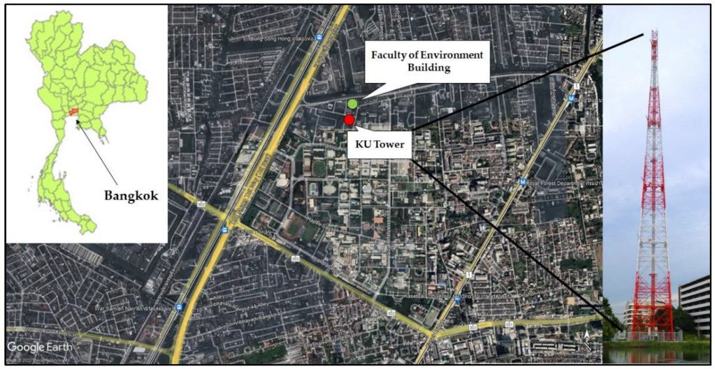
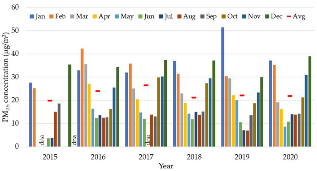
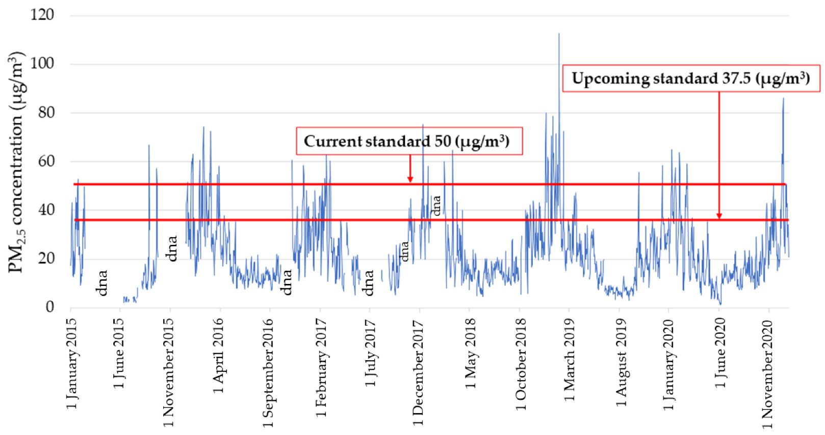
2.1. Site Description and Measuring Devices

The air pollution and meteorological data sampling site was the KU tower (13.85 °N, 100.57 °E) located at the Faculty of Environment, Kasetsart University (Figure 1). The tower is located in the northeast corner of the university campus, which is considered an urban–institutional area of the city, with major roads approximately several hundred meters from the measuring site. The measuring site is located on a flat area with the majority of surrounding land use within a 5-km radius being buildings and community land use (94%), with roads (4%) and water and other use types (2%) comprising the rest [29]. Considering that there are currently over 11.6 million vehicles registered in Bangkok (https://web.dlt.go.th/statistics/index.php, accessed on 25 February 2023), and with the addition of commuting vehicles, the impact of the traffic’s contribution to local PM_2.5 pollution is expected to be substantial.

Concentrations of fine particulate matter (PM_2.5, diameter < 2.5 μm; PM₁₀, diameter < 10 μm) were measured using the Tapered Element Oscillating Microbalance (TEOM) 1405 DF (Thermo Fisher Scientific Inc. Waltham, MA, USA). The instrument was located on the rooftop of the Faculty of Environment building at a height of 30 m and a distance of approximately 100 m from the Faculty of Environment building and the KU tower. There were no obstructions between the measuring sites that could affect data comparability.

The measured meteorological parameters included temperature, relative humidity (DMA875, LSI Lastem, Milano, Italy), wind speed and wind direction (DNA827, LSI Lastem, Milano, Italy), air pressure (DQA208, LSI Lastem, Milano, Italy) and precipitation (DQA130#C, LSI LASTEM, Milano, Italy). The latter was only measured 10 m AGL. We used data from long-term measurements of vertical meteorological factors at five heights above ground level (AGL)—10, 30, 50, 75, and 110 m—and PM_2.5 concentrations at 30 m AGL. All data used in this study were averaged over 1 h and collected and evaluated from 2015 to 2020.

2.2. PM_2.5 Prediction Process

The present study explored the applicability of machine learning (ML) in predicting PM_2.5 burden using open-source software (Weka 3.8.4, SourceForge, San Diego, CA, USA), comparing the performances of MLR and MLP models. Weka is a collection of machine learning algorithms for data mining and recognition tasks. The process includes methods and tools for data mining problems, such as regression, classification, clustering, association rule mining, and attribute selection [30].

This study aimed to apply the models to generate high-quality predictions for mass concentrations of local PM_2.5 at the measuring site days in advance and to verify the results using actual comprehensive long-term ambient meteorological and PM_2.5 data.

ML is a technique used to train computers (machines) to perform activities comparable to human understanding, such as learning from the past and making future predictions, faster and more objectively than an average human. The entire process can be described as follows: data collection and preparation, choice of model and its training, evaluation of model quality, and making predictions.

Here, the results of two supervised ML models, MLR and MLP, are presented. MLR determines whether there is a linear relationship between dependent and independent variables and predicts the value of the dependent variable using linear output functions. An extensive mathematical description and formulations of multivariate analysis methods are provided by Rencher and Christiansen [31].

MLP accepts multiple inputs through one or more input neurons and can learn complex decisions based on the weight of the data. It is a neural network in which input and output mapping is not necessarily linear. A recent report provides a good description of the processes and elementary steps involved in MLP modeling [32].

2.3. Validation Parameters

Pearson’s correlation coefficient (R), mean absolute error (MAE), and root mean square error (RMSE) were used to validate the computational results. R is a number between −1 and 1 that measures the strength and direction of the relationship between two variables. In correlation analysis, R > 0.7 describes a strong correlation, whereas R > 0.4 represents a moderate correlation. However, when appraising a correlation, it should be noted that the transition between correlation classes is not a step function.

$$\mathrm{R}=\frac{\sum (x_i-\stackrel{-}{x})(y_i-\stackrel{-}{y})}{\sqrt{\sum ({x_i-\stackrel{-}{x})}^2\sum {(y_i-\stackrel{-}{y})}^2}}$$

(1)

The mean absolute error (MAE) is a measure of the errors between observations and predictions, where $n$ is the number of testing samples, $x_i$ represents the observations, and $y_i$ represents the predictions.

$$\mathrm{MAE}=\frac{1}{n}{\sum }_{i=1}^n|y_i-x_i|$$

(2)

The root mean square error (RMSE) is sensitive to outliers. A smaller RMSE indicates better agreement between observations and predictions, higher prediction stability, and higher accuracy of the prediction model [33].

$$\mathrm{RMSE}=\sqrt{\frac{1}{n}{\sum }_{i=1}^n{(y_i-x_i)}^2}$$

(3)

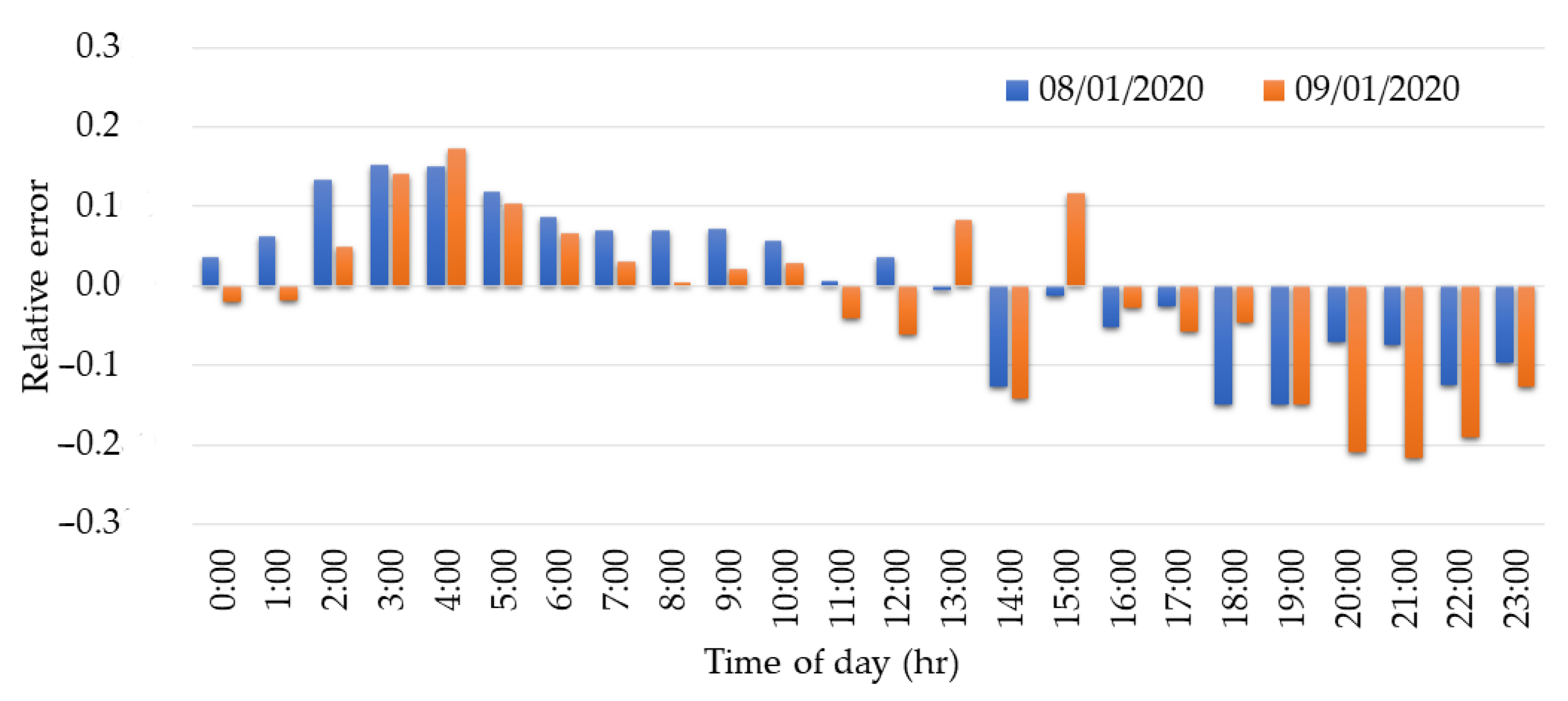
3. Results and Discussion

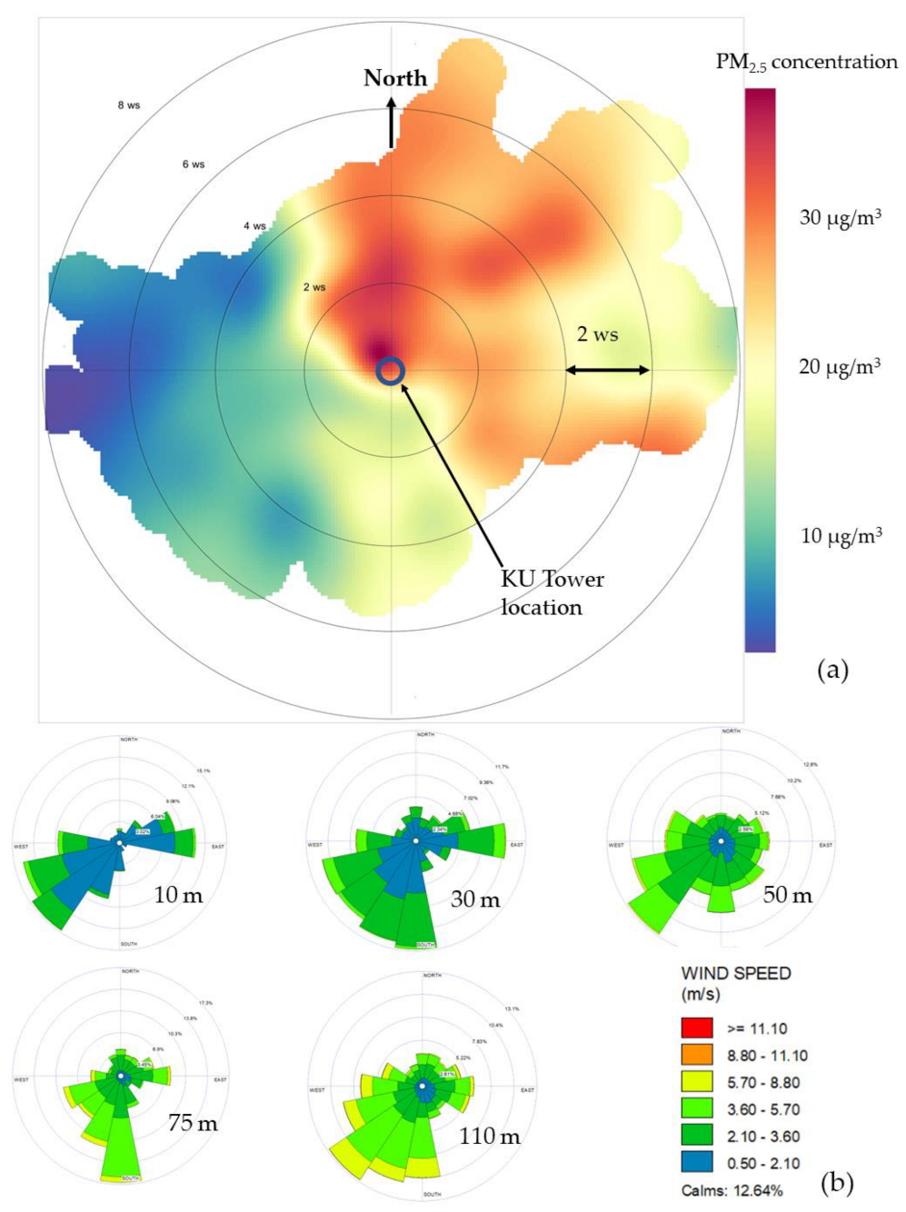
3.1. Relationship between PM_2.5 Concentration and Meteorological Factors

The PM_2.5 concentration was monitored continuously at a height of 30 m at the rooftop sampling site of the Faculty of Environment, Kasetsart University, Bangkok, Thailand. The data shown in Figure 2 encompassed a period of 6 years, from 2015 to 2020. The presented monthly averages showed a distinct pattern, with a mid-year minimum and the highest concentrations typically from November to March. Based on the stricter, recently published upcoming Thailand national annual PM_2.5 standard (15 µg/m³), it is evident that the annual average PM_2.5 concentrations at the measuring site have been exceeded since 2015. Applying the current Thailand national annual PM_2.5 standard (25 µg/m³), which was valid at the time of data acquisition, provides an administratively acceptable picture; however, the worrying environmental situation proves the appropriateness of the new standard.

Analysis of month-by-month PM_2.5 averages over the investigated period (2015–2020) shows that the mass concentrations in January, February, March, November, and December exceeded the Thai national annual PM_2.5 standard (25 µg/m³), and the best air quality was recorded in June–August. Based on the new annual PM_2.5 standard (15 µg/m³), the air quality from 2015 to 2020 met the permissible requirements during the period from May to September, except in the year 2019. PM_2.5 concentrations exceeded the current short-term standard (50 µg/m³ within 24 h) in January 2019, consistent with earlier findings [34].

Some data for the years 2015 and 2017 were unavailable due to equipment maintenance and are denoted as “dna” or “data not available” in Figure 2. These only negligibly impacted the ML process. The overall morphology of data distribution (Figure 2) shows a typical U-shaped form for Southeast Asia, with the lowest ambient PM_2.5 concentrations recorded in July and August. Day-by-day PM_2.5 concentration data from 2015 to 2020 (Figure 3) show that the current daily PM_2.5 standard (50 µg/m³) was exceeded on 4 days in 2015, 28 days in 2016, 10 days in 2017, 10 days in 2018, 16 days in 2019, and 21 days in 2020. The upcoming daily PM_2.5 standard of 37.5 µg/m³ was exceeded within 24 h on 18 days in 2015, 51 days in 2016, 42 days in 2017, 35 days in 2018, 38 days in 2019, and 52 days in 2020.

Meteorological factors such as wind speed and wind direction determine the levels and spatial distribution of PM_2.5 in the vicinity of the measuring site. Using data from 2015 to 2020, spatial dispersion and PM_2.5 concentrations around the KU tower measured at a height of 30 m were modeled using RStudio software [35]. The results are shown in Figure 4a using a polar plot. A distinct pattern showing PM_2.5 concentration gradients from northeast to southwest can be observed and is understandable considering the wind direction and wind speed at various levels, from 10 to 110 m above ground level (Figure 4b). It must be mentioned that in the zone between the ground and the undisturbed wind flow, the wind experiences friction depending on the surface structure. Within the urban area, its speed decreases more abruptly, but its turbulence increases. In general, it can be estimated that ground wind velocity decreases to approximately 15% in relation to the undisturbed flow [36]. However, currently, the computations and air quality predictions in this work relate to a height of 30 m above the ground owing to the availability of PM_2.5 emission data needed to verify the quality of predictions.

The correlations between PM_2.5 concentrations and meteorological factors such as wind speed (WS) (R = −0.148), temperature (T) (R = −0.141), relative humidity (RH) (R = −0.219), barometric pressure (BP) (R = 0.415), and rain (R = −0.046) averaged from 2015 to 2020 are presented in

Table 1. Correlations between PM_2.5 concentration and meteorological factors obtained at a height of 30 m from 2015 to 2020.

All Seasons	WS	WD	T	RH	BP	Rain	PM2.5
WS (m/s)	1.000
WD (°)	0.003	1.000
T (°C)	0.151	0.177	1.000
RH (%)	−0.324	0.024	−0.540	1.000
BP (hPa)	−0.208	−0.321	−0.442	−0.043	1.000
Rain (mm)	0.015	0.010	−0.092	0.122	−0.039	1.000
PM2.5 (µg/m3)	−0.148	−0.142	−0.141	−0.219	0.415	−0.046	1.000

. The results show that wind speed, temperature, relative humidity, and rain are inversely correlated with PM_2.5 concentration. Apparently, the main factor affecting PM_2.5 was barometric pressure (R = 0.415) rather than wind. Local PM_2.5 concentrations have a general tendency to increase due to increasing barometric pressure. This condition is not beneficial for the dilution and spatial diffusion of pollutants and thus increases the local PM_2.5 concentration. Similar results have been reported previously [37].

Table 2. Seasonal variations in the correlations between PM_2.5 concentration and meteorological factors obtained at a height of 30 m from 2015 to 2020.

Winter Season	WS	WD	T	RH	BP	Rain	PM2.5
WS (m/s)	1.000
WD (°)	−0.246	1.000
T (°C)	−0.001	0.027	1.000
RH (%)	−0.301	0.120	−0.421	1.000
BP (hPa)	0.094	−0.145	−0.515	0.037	1.000
Rain (mm)	−0.009	0.015	−0.024	0.060	0.000	1.000
PM2.5 (µg/m3)	−0.214	0.115	−0.147	−0.004	0.154	−0.020	1.000
Summer season	WS	WD	T	RH	BP	Rain	PM2.5
WS (m/s)	1.000
WD (°)	0.076	1.000
T (°C)	0.224	0.254	1.000
RH (%)	−0.253	−0.196	−0.856	1.000
BP (hPa)	−0.417	−0.106	−0.484	0.339	1.000
Rain (mm)	0.001	−0.012	−0.105	0.079	0.019	1.000
PM2.5 (µg/m3)	0.091	−0.030	0.099	−0.261	−0.010	−0.023	1.000
Rainy season	WS	WD	T	RH	BP	Rain	PM2.5
WS (m/s)	1.000
WD (°)	0.273	1.000
T (°C)	0.294	0.229	1.000
RH (%)	−0.464	−0.366	−0.877	1.000
BP (hPa)	−0.413	−0.172	−0.322	0.355	1.000
Rain (mm)	0.020	−0.034	−0.163	0.146	0.010	1.000
PM2.5 (µg/m3)	−0.176	−0.157	0.072	0.020	0.118	0.006	1.000

shows the correlations between average PM_2.5 concentrations and meteorological factors segregated by seasons: winter (mid-October to February), summer (March to mid-May), and the rainy season (mid-May to Mid-October). In the winter season, the correlation with wind speed was higher than with the other meteorological factors (R = −0.214), with a remarkable influence of barometric pressure. In the summer season, correlation with relative humidity was higher than with the other meteorological factors (R = −0.261). In the rainy season, the correlation between wind speed and wind direction was higher than with the other meteorological factors; however, the influence of barometric pressure was still remarkable, indicating the strength of convective inhibition in the atmosphere.

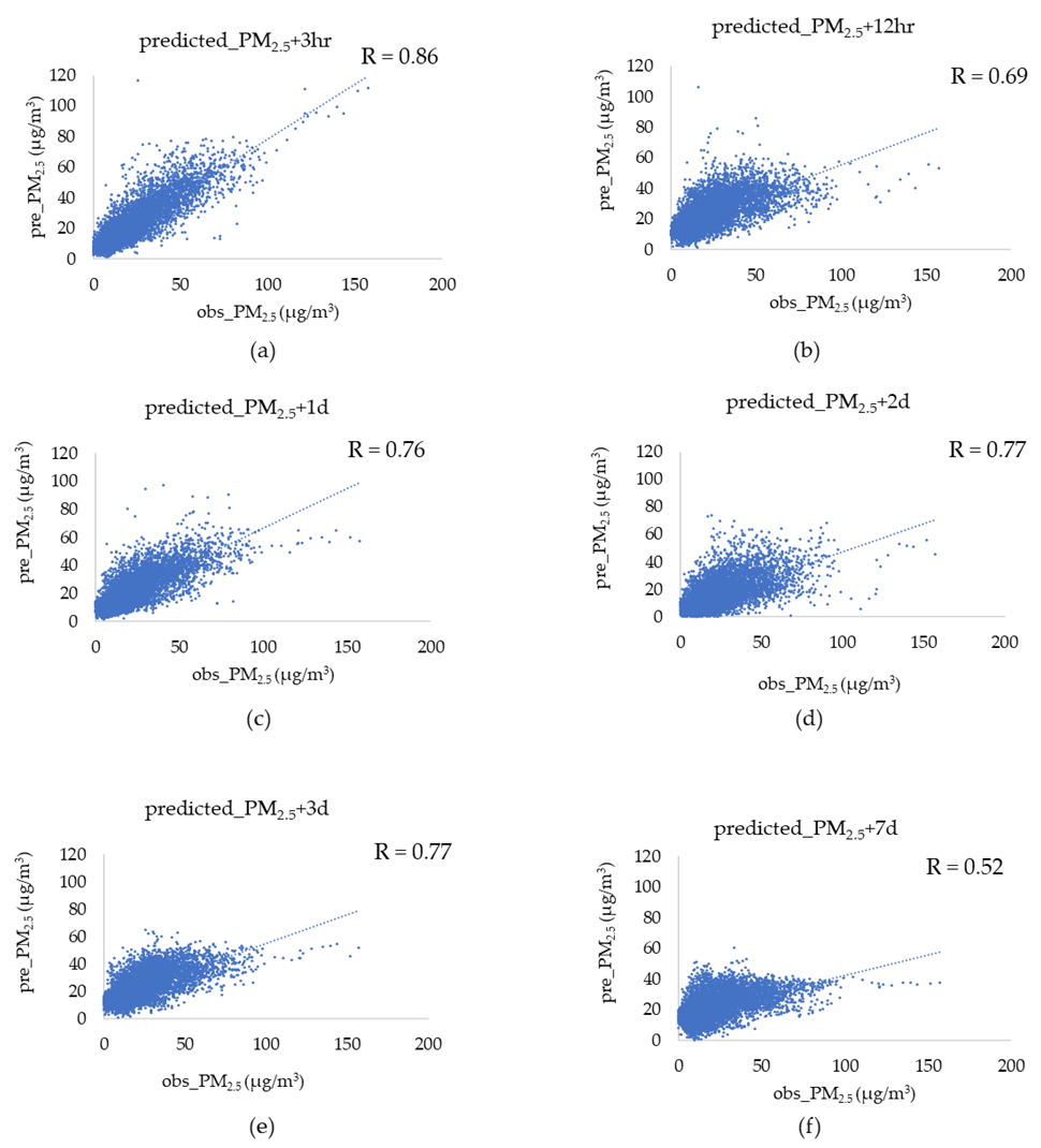
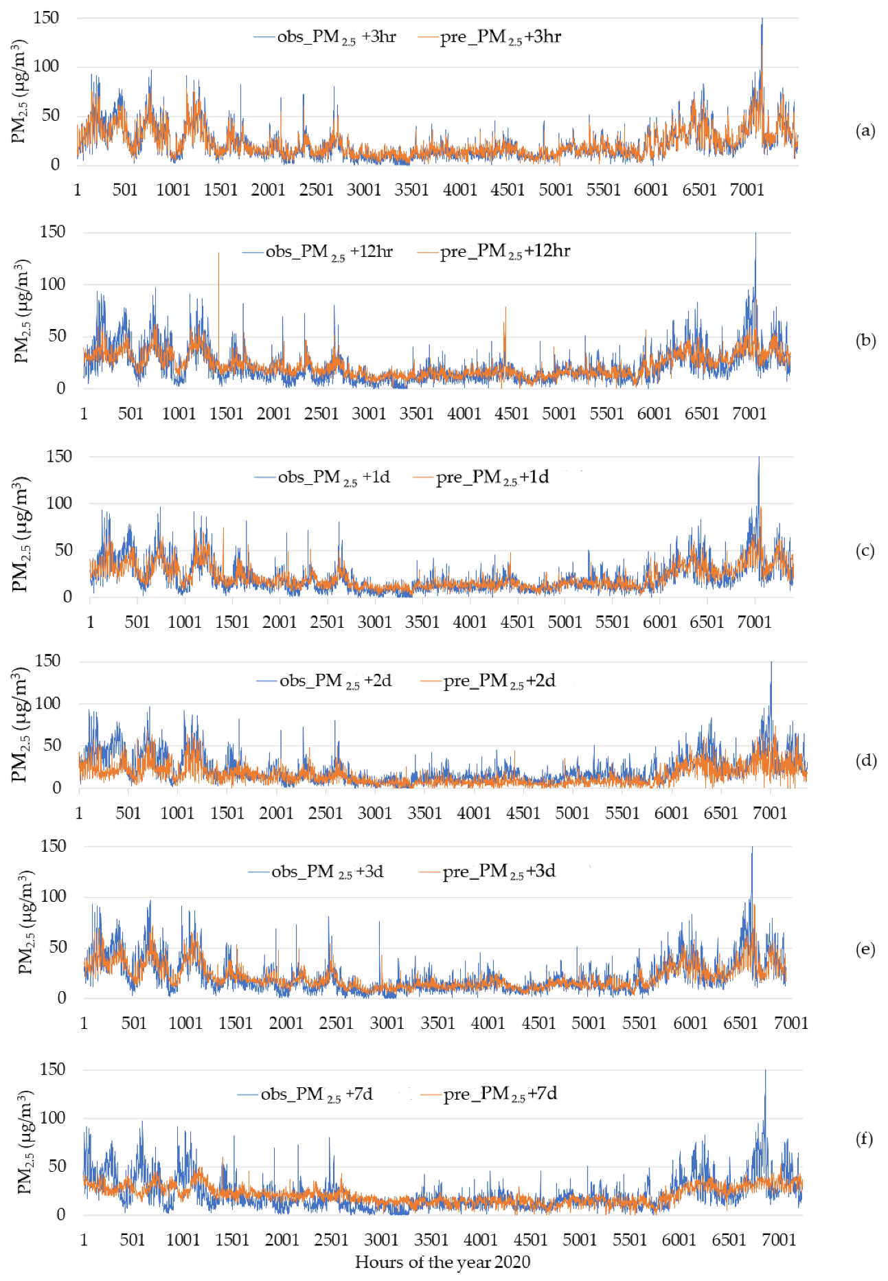
3.2. Ambient Concentrations of PM_2.5 Predicted Using Multiple Linear Regression (MLR)

Using the meteorological factors acquired five levels above the ground at the KU tower, the MLR model was trained and used for the prediction of PM_2.5 concentrations under six scenarios: 3 h, 12 h, 1 day, 2 days, 3 days, and 7 days ahead. The results of these predictions are shown in Figure 5. For the 3- and 12-hour scenarios, very good correlations (R = 0.86 and 0.69, respectively) were achieved between the observed and predicted data. Moreover, a strong-to-moderate relationship was found for the other scenarios of 1 day, 2 days, 3 days, and 7 days ahead, with R = 0.76, 0.77, 0.77, and 0.52, respectively. Using this approach, time series of PM_2.5 concentrations for the year 2020 were predicted and compared with the actual data (Figure 6). The x-axis represents the hours of the year. The first 2000 h correspond approximately to the months of January–March 2020.

Good agreement in the time series for the short time ahead and the 1 day ahead was evident. For the 2- and 3-days-ahead conditions, the overall agreement between the measurement and the prediction was reasonable, confirming general concentration trends; however, the predicted values recurrently underestimated the PM_2.5 level, similar to a previous report [34], which can be linked to varying meteorological conditions.

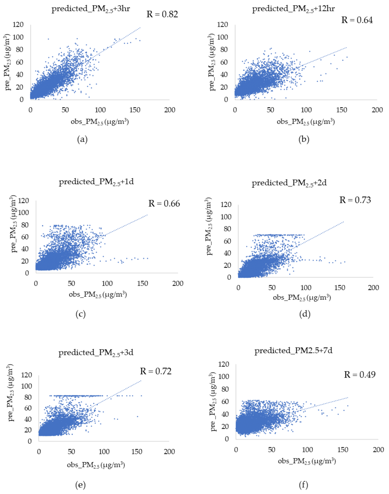
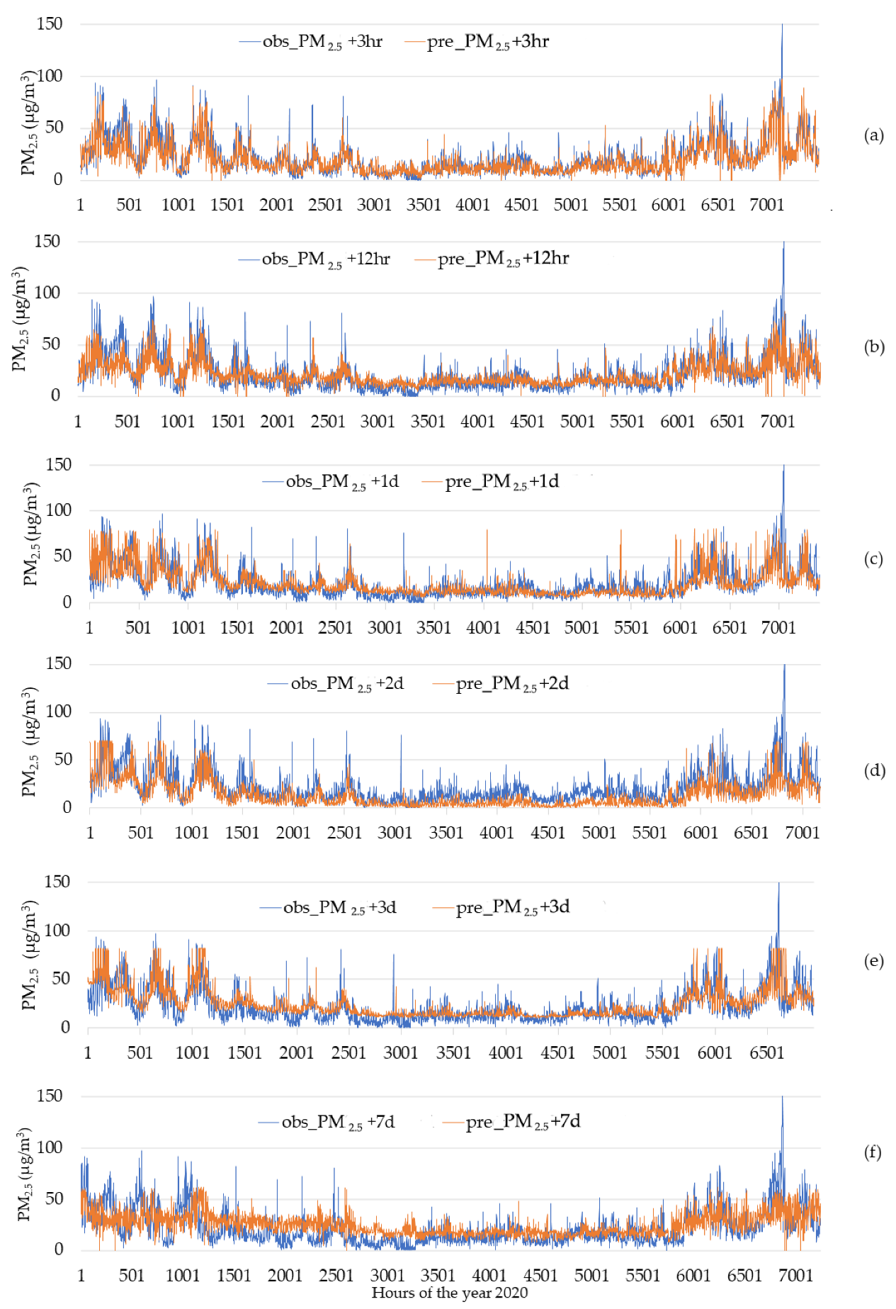
3.3. Ambient Concentrations of PM_2.5 Predicted Using Multilayer Perceptron (MLP)

In another model, a neural network was developed using a multilayer perceptron (MLP) approach. The results of the PM_2.5 prediction are shown in Figure 7. For the short-term scenario, a very strong correlation (R = 0.82) was obtained between the measured and predicted data. With the exception of the 1-day ahead scenario, which showed a moderately strong relationship (R = 0.66) between the observed and predicted PM_2.5 concentrations, the scenarios for predictions 2 and 3 days ahead showed very strong correlations, with R = 0.73 and 0. 72, respectively. However, it must be noted that the prediction of PM_2.5 concentrations using MLP occasionally exhibited limiting values, particularly visible in Figure 7e, likely from bias that was introduced during the learning process to rectify the errors of the training and data normalization [38]. However, the prediction bias did not determinedly influence the trend of PM_2.5 concentration prediction for the year 2020, as shown in Figure 8, and overall agreement and mirroring of the general trends in the data morphology were unmistakable.

3.4. Comparison between MLR and MLP Techniques

The main aim of the training process of machine learning is to optimize the models for predicting the dependent variable and reducing errors. To assess the performance of the predicting models, the mean absolute errors (MAE) and root mean squared error (RMSE), together with the correlation coefficients (R) for the MLR and MLP models and various prediction scenarios are summarized in

Table 3. Statistical results of the assessment of the accuracy of multilayer perceptron (MLP) and multiple linear regression (MLR) models.

	Conditions	Ahead 3 h		Ahead 12 h		Ahead 24 h		Ahead 48 h		Ahead 72 h		Ahead 7 Days
Statistics		MLP	MLR	MLP	MLR	MLP	MLR	MLP	MLR	MLP	MLR	MLP	MLR
Correlation coefficient (R)		0.82	0.86	0.64	0.69	0.66	0.76	0.73	0.77	0.72	0.77	0.49	0.52
Mean absolute error (MAE)		6.62	6.00	9.08	8.47	8.68	7.54	10.67	7.54	8.84	7.69	11.62	10.39
Root mean squared error (RMSE)		9.92	8.68	12.86	12.14	13.01	11.07	14.55	10.98	12.35	11.02	15.27	14.43

. Both statistical indicators (MAE and RMSE) denote the solid quality of the prediction data. The decision on which indicator is more advantageous is not immediately clear and would also depend on the distribution of actual data. MAE assigns the same importance to each error, whereas RMSE emphasizes the largest errors and is more sensitive to outliers. Here, the training was directed toward optimizing both indicators applied to the MLR and MLP models, as shown in Table 3. It is evident that although errors increased with prediction over a longer time, reasonable values of forward predictions were obtained for up to 7 days. Based on the obtained results, the preference for MLR was determined. This was confirmed using recently published data from Northern Thailand [39].

Finally, the MLR model of the 1 day ahead scenario was used to verify the usefulness of the modeling approach, emphasizing the hour-by-hour quality of the prediction of PM_2.5 burden for two selected days: 8th and 9th of January 2020. These days were chosen because of the PM_2.5 concentrations that exceeded the Thai ambient air quality standard without precipitation. The daily averaged vertical meteorological parameters used for PM_2.5 prediction were temperature (29.5 °C, 30.2 °C), relative humidity (56.3%, 58.1%), barometric pressure (1008.9 hPa, 1008.3 hPa), and wind speed (1.7 m/s, 1.3 m/s) for both days, respectively. The prevailing wind direction was northeast. Figure 9 shows the relative error ((x_obs/x_pred) − 1) between the actual and observed data. The predicted data for the PM_2.5 concentrations were not constant during the 24-h period and varied as a function of time, but only within +/− 20%, thus proving the quality of modeling.

4. Conclusions

Predicting air quality is a challenging task because of the dynamics of the atmosphere and the spatiotemporal variability of air pollutants. The consequences of air pollution necessitate constant and reliable air quality monitoring and are particularly important in locations where the number of monitoring stations is limited [40]. Complementary to conventional measurements, advanced prediction of upcoming pollution and excess PM_2.5 concentration episodes using machine learning techniques based on meteorological parameters has become an increasingly important tool for early warning systems and preventive measures.

In this study, two different models, MLR and MLP, were selected and the software Weka 3.8.4 was trained to forecast the expected PM_2.5 level up to 7 days in advance. As a reference, data from long-term measurements of meteorological factors and PM_2.5 concentrations (years 2015–2020) were used. MLP and MLR were compared to determine the quality of the predictions and assessment of the errors. Despite the differences between the models, their predictions were comparable and stable. Predicting up to 7 days ahead was therefore proven to be possible and reliable. Exploiting a particular 2-day period as an example showed that even an hour-by-hour prediction of PM_2.5 concentrations within an error of less than 20% was possible. Thus, the feasibility of PM_2.5 prediction using ML has been proven. The results were obtained from data collected 30 m AGL, and this was dictated by the availability of experimental data needed for verification of the computed results. Considering that within urban areas air movement due to wind speed reduces rather abruptly while its turbulence increases, an assumption of homogenously mixed PM_2.5 burden within the urban dome seems feasible. The findings presented here indicate the importance of this research and its applicability as an early warning system for better air quality management in urban areas.

References

1. Nazarenko, Y.; Pal, D.; Ariya, P.A. Air quality standards for the concentration of particulate matter 2.5, global descriptive analysis. Bull. World Health Organ. 2021, 99, 125D–137D. [Google Scholar] [CrossRef] [PubMed]
2. Cohen, A.J.; Brauer, M.; Burnett, R.; Anderson, H.R.; Frostad, J.; Estep, K.; Balakrishnan, K.; Brunekreef, B.; Dandona, L.; Dandona, R.; et al. Estimates and 25-year trends of the global burden of disease attributable to ambient air pollution: An analysis of data from the Global Burden of Diseases Study 2015. Lancet 2017, 389, 1907–1918. [Google Scholar] [CrossRef] [Green Version]
3. The Lancet, E. Air pollution—Time to address the silent killer. Lancet Respir. Med. 2021, 9, 1203. [Google Scholar] [CrossRef]
4. Narita, D.; Oanh, N.; Sato, K.; Huo, M.; Permadi, D.; Chi, N.; Ratanajaratroj, T.; Pawarmart, I. Pollution Characteristics and Policy Actions on Fine Particulate Matter in a Growing Asian Economy: The Case of Bangkok Metropolitan Region. Atmosphere 2019, 10, 227. [Google Scholar] [CrossRef] [Green Version]
5. Sun, X.; Zhao, T.; Tang, G.; Bai, Y.; Kong, S.; Zhou, Y.; Hu, J.; Tan, C.; Shu, Z.; Xu, J.; et al. Vertical changes of PM2.5 driven by meteorology in the atmospheric boundary layer during a heavy air pollution event in central China. Sci. Total Environ. 2023, 858, 159830. [Google Scholar] [CrossRef] [PubMed]
6. Acevedo, O.C.; Degrazia, G.A.; Puhales, F.S.; Martins, L.G.N.; Oliveira, P.E.S.; Teichrieb, C.; Silva, S.M.; Maroneze, R.; Bodmann, B.; Mortarini, L.; et al. Monitoring the Micrometeorology of a Coastal Site next to a Thermal Power Plant from the Surface to 140 m. Bull. Am. Meteorol. Soc. 2018, 99, 725–738. [Google Scholar] [CrossRef]
7. Gazette, R.T.G. Announcement of the National Environment Board Subject: Setting the Standard for Dust Particles with a Size not Exceeding 2.5 Micrometers in the General Atmosphere. Available online: https://thainews.prd.go.th/en/news/detail/TCATG220715124733629 (accessed on 15 July 2022).
8. Chuersuwan, N.; Nimrat, S.; Lekphet, S.; Kerdkumrai, T. Levels and major sources of PM2.5 and PM10 in Bangkok Metropolitan Region. Environ. Int. 2008, 34, 671–677. [Google Scholar] [CrossRef] [PubMed]
9. Chirasophon, S.; Pochanart, P. The Long-term Characteristics of PM10 and PM2.5 in Bangkok, Thailand. Asian J. Atmos. Environ. 2020, 14, 73–83. [Google Scholar] [CrossRef] [Green Version]
10. Alas, H.D.; Stocker, A.; Umlauf, N.; Senaweera, O.; Pfeifer, S.; Greven, S.; Wiedensohler, A. Pedestrian exposure to black carbon and PM2.5 emissions in urban hot spots: New findings using mobile measurement techniques and flexible Bayesian regression models. J. Expo. Sci. Environ. Epidemiol. 2022, 32, 604–614. [Google Scholar] [CrossRef] [PubMed]
11. Pozzer, A.; Anenberg, S.C.; Dey, S.; Haines, A.; Lelieveld, J.; Chowdhury, S. Mortality Attributable to Ambient Air Pollution: A Review of Global Estimates. Geohealth 2023, 7, e2022GH000711. [Google Scholar] [CrossRef]
12. Kumar, S.; Mishra, S.; Singh, S.K. A machine learning-based model to estimate PM2.5 concentration levels in Delhi’s atmosphere. Heliyon 2020, 6, e05618. [Google Scholar] [CrossRef] [PubMed]
13. Winalai, C.; Nanthasen, S.; Chadsuthi, S. The effect of weather on PM2.5 in Bangkok area and Bangkok metropolitan region using machine learning. Life Sci. Environ. J. 2022, 23, 409–421. [Google Scholar] [CrossRef]
14. Lin, L.; Liang, Y.; Liu, L.; Zhang, Y.; Xie, D.; Yin, F.; Ashraf, T. Estimating PM2.5 Concentrations Using the Machine Learning RF-XGBoost Model in Guanzhong Urban Agglomeration, China. Remote Sens. 2022, 14, 5239. [Google Scholar] [CrossRef]
15. Cabaneros, S.M.; Calautit, J.K.; Hughes, B.R. A review of artificial neural network models for ambient air pollution prediction. Environ. Model. Softw. 2019, 119, 285–304. [Google Scholar] [CrossRef]
16. Chen, J.; de Hoogh, K.; Gulliver, J.; Hoffmann, B.; Hertel, O.; Ketzel, M.; Bauwelinck, M.; van Donkelaar, A.; Hvidtfeldt, U.A.; Katsouyanni, K.; et al. A comparison of linear regression, regularization, and machine learning algorithms to develop Europe-wide spatial models of fine particles and nitrogen dioxide. Environ. Int. 2019, 130, 104934. [Google Scholar] [CrossRef]
17. Chu, Y.; Liu, Y.; Li, X.; Liu, Z.; Lu, H.; Lu, Y.; Mao, Z.; Chen, X.; Li, N.; Ren, M.; et al. A Review on Predicting Ground PM2.5 Concentration Using Satellite Aerosol Optical Depth. Atmosphere 2016, 7, 129. [Google Scholar] [CrossRef] [Green Version]
18. Miskell, G.; Pattinson, W.; Weissert, L.; Williams, D. Forecasting short-term peak concentrations from a network of air quality instruments measuring PM2.5 using boosted gradient machine models. J. Environ. Manag. 2019, 242, 56–64. [Google Scholar] [CrossRef]
19. Kleine Deters, J.; Zalakeviciute, R.; Gonzalez, M.; Rybarczyk, Y. Modeling PM2.5 Urban Pollution Using Machine Learning and Selected Meteorological Parameters. J. Electr. Comput. Eng. 2017, 2017, 5106045. [Google Scholar] [CrossRef] [Green Version]
20. Gaudart, J.; Giusiano, B.; Huiart, L. Comparison of the performance of multi-layer perceptron and linear regression for epidemiological data. Comput. Stat. Data Anal. 2004, 44, 547–570. [Google Scholar] [CrossRef] [Green Version]
21. Arsov, M.; Zdravevski, E.; Lameski, P.; Corizzo, R.; Koteli, N.; Mitreski, K.; Trajkovik, V. Short-term air pollution forecasting based on environmental factors and deep learning models. In Proceedings of the 2020 Federated Conference on Computer Science and Information Systems, Sofia, Bulgaria, 6–9 September 2020; pp. 15–22. [Google Scholar] [CrossRef]
22. Zhang, Z.; Zeng, Y.; Yan, K. A hybrid deep learning technology for PM2.5 air quality forecasting. Environ. Sci. Pollut. Res. Int. 2021, 28, 39409–39422. [Google Scholar] [CrossRef]
23. Ke, H.; Gong, S.; He, J.; Zhang, L.; Cui, B.; Wang, Y.; Mo, J.; Zhou, Y.; Zhang, H. Development and application of an automated air quality forecasting system based on machine learning. Sci. Total Environ. 2022, 806, 151204. [Google Scholar] [CrossRef] [PubMed]
24. Raffee, A.F.; Rahmat, S.N.; Hamid, H.A.; Jaffar, M.I. A Review on Short-Term Prediction of Air Pollutant Concentrations. Int. J. Eng. Technol. 2018, 7, 32–35. [Google Scholar] [CrossRef] [Green Version]
25. Zong, R.H.; Zhang, T.Y.; Chen, Z.; Zhu, Y. Cross-city PM2.5 predictions with recurrent neural network. IOP Conf. Ser. Earth Environ. Sci. 2019, 291, 012002. [Google Scholar] [CrossRef] [Green Version]
26. Bera, B.; Bhattacharjee, S.; Sengupta, N.; Saha, S. PM2.5 concentration prediction during COVID-19 lockdown over Kolkata metropolitan city, India using MLR and ANN models. Environ. Chall. 2021, 4, 100155. [Google Scholar] [CrossRef]
27. Shah, J.; Mishra, B. Analytical equations based prediction approach for PM2.5 using artificial neural network. SN Appl. Sci. 2020, 2, 1516. [Google Scholar] [CrossRef]
28. Zheng, Y.; Zhang, Q.; Wang, Z.; Zhu, Y. Application research on PM2.5 concentration prediction of multivariate chaotic time series. IOP Conf. Ser. Earth Environ. Sci. 2019, 237, 022010. [Google Scholar] [CrossRef]
29. Choomanee, P.; Bualert, S.; Thongyen, T.; Salao, S.; Szymanski, W.W.; Rungratanaubon, T. Vertical Variation of Carbonaceous Aerosols with in the PM2.5 Fraction in Bangkok, Thailand. Aerosol. Air Qual. Res. 2020, 20, 43–52. [Google Scholar] [CrossRef] [Green Version]
30. Eibe, F.; Mark, A.H.; Ian, H.W. WEKA workbench. In Data Mining: Practical Machine Learning Tools and Techniques; Morgan Kaufmann: Burlington, MA, USA, 2016. [Google Scholar]
31. Rencher, A.C.; Christensen, W.F. Methods of Multivariate Analysis; Wiley Series in Probability and Statistics; John Wiley & Sons: New, York, NY, USA, 2012. [Google Scholar]
32. Hoffman, S.; Jasiński, R. The Use of Multilayer Perceptrons to Model PM2.5 Concentrations at Air Monitoring Stations in Poland. Atmosphere 2023, 14, 96. [Google Scholar] [CrossRef]
33. Zhang, Q.; Wu, S.; Wang, X.; Sun, B.; Liu, H. A PM2.5 concentration prediction model based on multi-task deep learning for intensive air quality monitoring stations. J. Clean. Prod. 2020, 275, 122722. [Google Scholar] [CrossRef]
34. Miao, Y.; Liu, S.; Guo, J.; Yan, Y.; Huang, S.; Zhang, G.; Zhang, Y.; Lou, M. Impacts of meteorological conditions on wintertime PM2.5 pollution in Taiyuan, North China. Environ. Sci. Pollut. Res. Int. 2018, 25, 21855–21866. [Google Scholar] [CrossRef]
35. Team, R. RStudio: Integrated Development for R; Rstudio: Boston, MA, USA, 2020. [Google Scholar]
36. Tahbaz, M. Estimation of the Wind Speed in Urban Areas—Height Less than 10 Metres. Int. J. Vent. 2016, 8, 75–84. [Google Scholar] [CrossRef]
37. Li, X.; Feng, Y.J.; Liang, H.Y. The Impact of Meteorological Factors on PM2.5 Variations in Hong Kong. IOP Conf. Ser. Earth Environ. Sci. 2017, 78, 012003. [Google Scholar] [CrossRef]
38. Bekesiene, S.; Meidute-Kavaliauskiene, I. Artificial Neural Networks for Modelling and Predicting Urban Air Pollutants: Case of Lithuania. Sustainability 2022, 14, 2470. [Google Scholar] [CrossRef]
39. Amnuaylojaroen, T. Prediction of PM2.5 in an Urban Area of Northern Thailand Using Multivariate Linear Regression Model. Adv. Meteorol. 2022, 2022, 3190484. [Google Scholar] [CrossRef]
40. Li, X.; Jin, L.; Kan, H. Air pollution: A global problem needs local fixes. Nature 2019, 570, 437–439. [Google Scholar] [CrossRef] [Green Version]
Figure 1. Location of data acquisition instruments at Kasetsart University, Bangkok, Thailand.
Atmosphere 14 00589 g001
Figure 2. Monthly averages (vertical bars) and annual averages (horizontal bars) of PM2.5 concentrations from 2015 to 2020 measured at Kasetsart University using TEOM.
Atmosphere 14 00589 g002
Figure 3. Daily averages (over 24 h) of PM2.5 concentrations from 2015 to 2020 obtained at Kasetsart University using TEOM. Some days are missing data due to equipment maintenance.
Atmosphere 14 00589 g003
Figure 4. Polar plot of actual PM2.5 concentrations measured at 30 m (a), averaged over the years 2015–2020, and the corresponding wind direction and wind speed distribution measured at the KU tower at the indicated levels (b).
Atmosphere 14 00589 g004
Figure 5. Quality of predictions (R) of PM2.5 concentrations for up to 7 days using multiple linear regression compared with observed PM2.5 data. Forward prediction for: (a) 3 h, (b) 12 h, (c) 1 day, (d) 2 days, (e) 2 days, (f) 7 days.
Atmosphere 14 00589 g005
Figure 6. Measured and predicted PM2.5 concentrations obtained using multiple linear regression modeling. Forward prediction for: (a) 3 h, (b) 12 h, (c) 1 day, (d) 2 days, (e) 2 days, (f) 7 days.
Atmosphere 14 00589 g006
Figure 7. Quality of prediction (R) of PM2.5 concentrations for up to 7 days using the multilayer perceptron approach compared with observed PM2.5 data. Forward prediction for: (a) 3 h, (b) 12 h, (c) 1 day, (d) 2 days, (e) 2 days, (f) 7 days.
Atmosphere 14 00589 g007
Figure 8. Variations between observed PM2.5 concentrations and PM2.5 concentrations predicted using the multilayer perceptron method. Forward prediction for: (a) 3 h, (b) 12 h, (c) 1 day, (d) 2 days, (e) 2 days, (f) 7 days.
Atmosphere 14 00589 g008
Figure 9. Relative error between predicted PM2.5 concentrations and those observed on 8 January and 9 January 2020, showing the accuracy of the developed method as a function of time.
Atmosphere 14 00589 g009