

Applying Bayesian Models to Reduce Computational Requirements of Wildfire Sensitivity Analyses


Abstract
1. Introduction
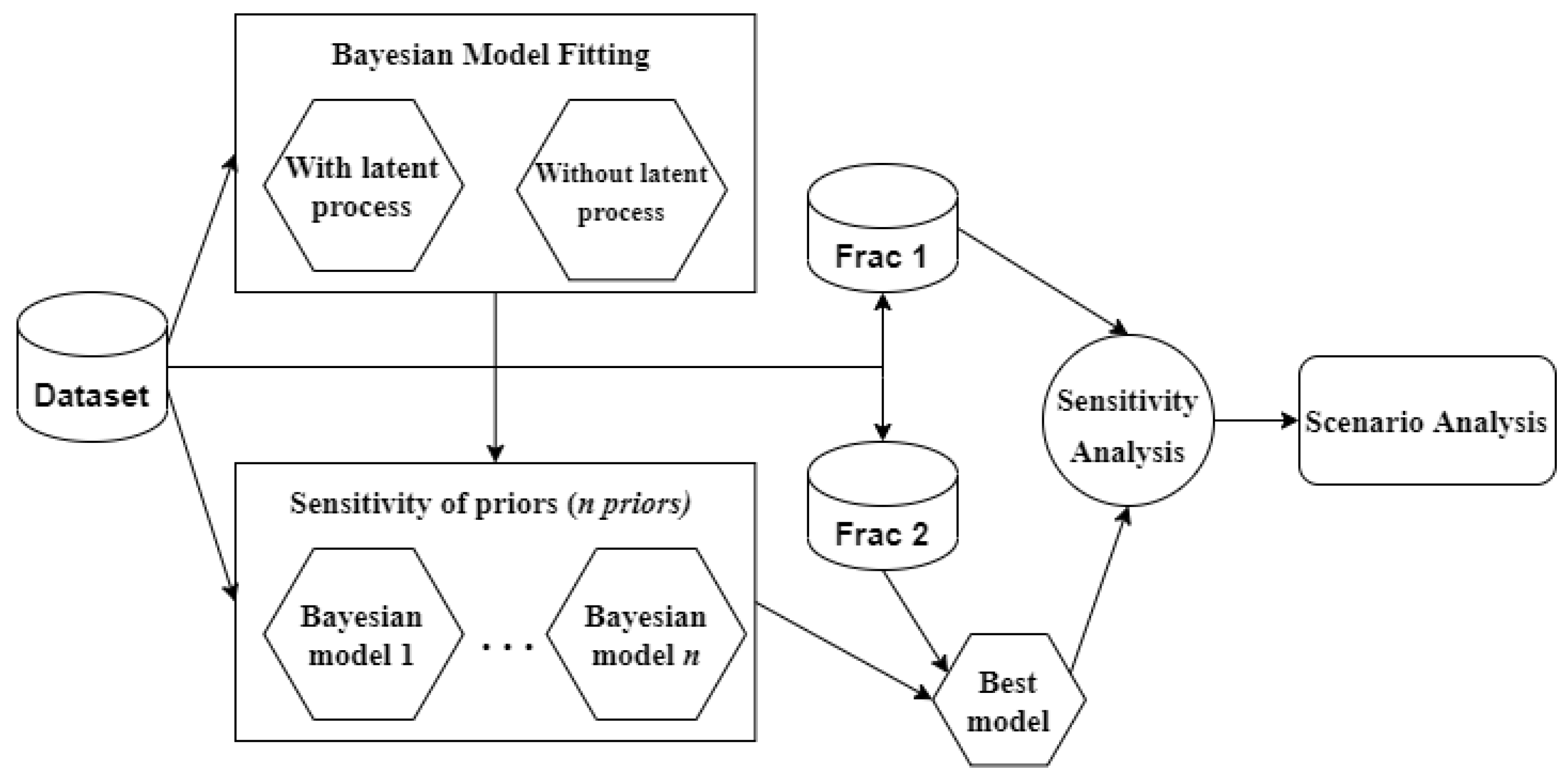
2. Workflow
2.1. Bayesian Model Fitting
2.1.1. Influence of Latent Process
2.1.2. Sensitivity to the Priors
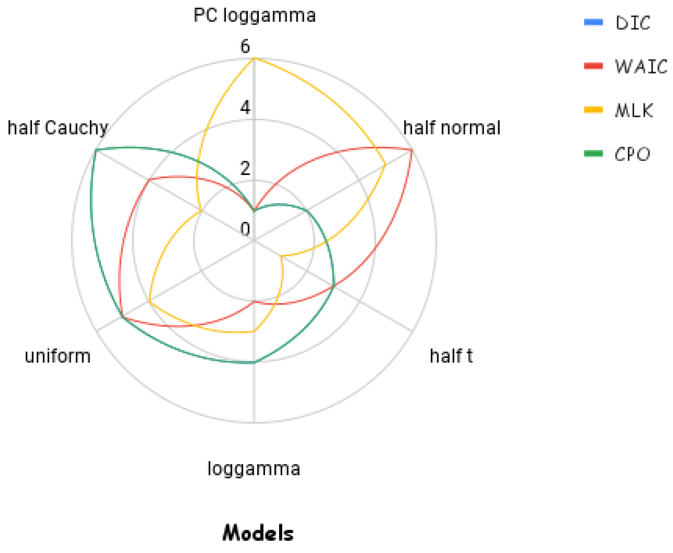
2.1.3. Evaluation Metrics
3. Experimental Setup
3.1. Fire Simulation Tool—Spark
3.2. Weather Inputs
3.3. Wildfire Management Practice Use Case—Scenario Analysis
3.3.1. Study Area
3.3.2. Sensitivity Analysis
3.3.3. Evaluation Metrics
4. Results and Discussion
4.1. Model Fitting
4.1.1. Latent Effects
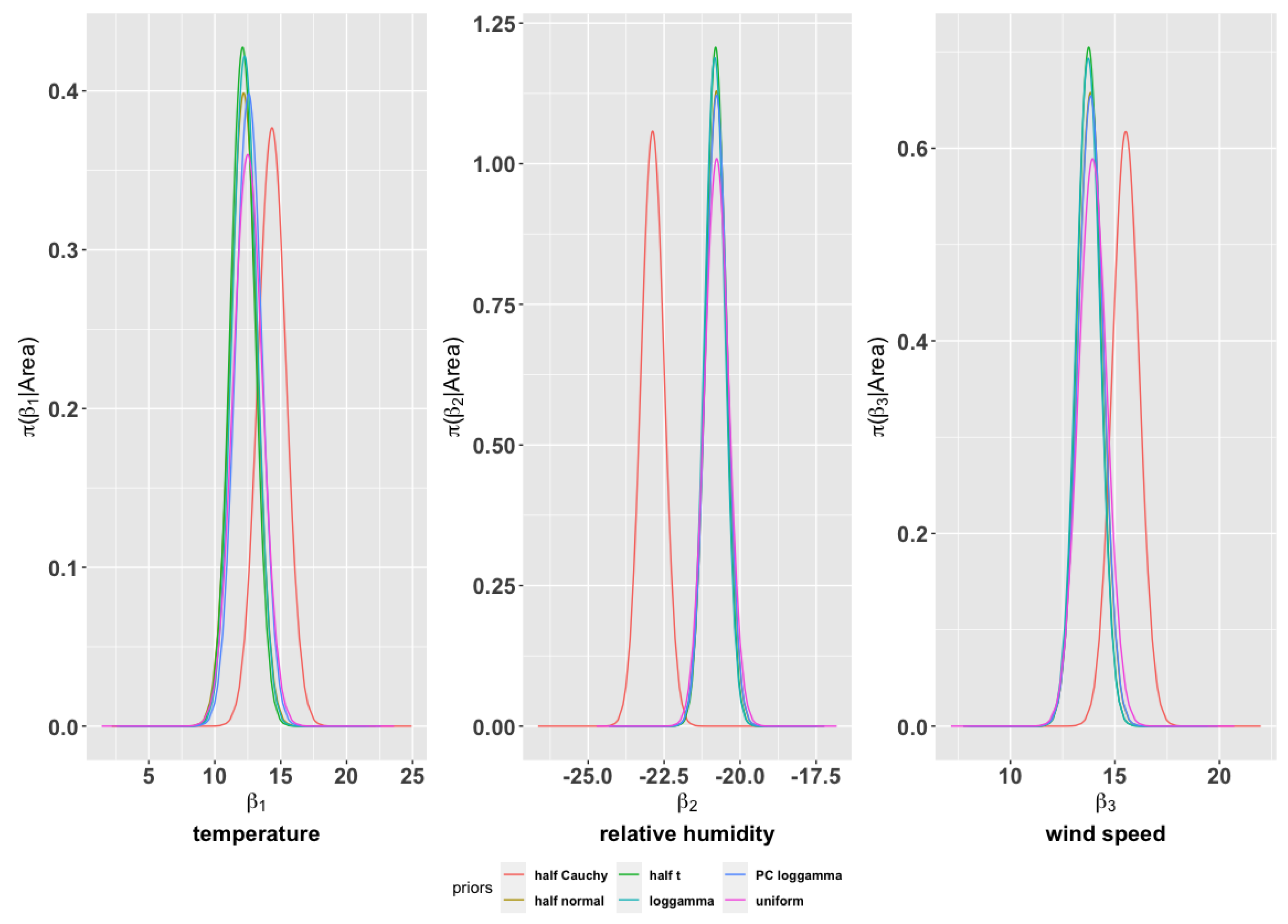
4.1.2. Sensitivity of Bayesian Modeling to Priors
4.2. Wildfire Management Practice Use Case—Scenario Analysis
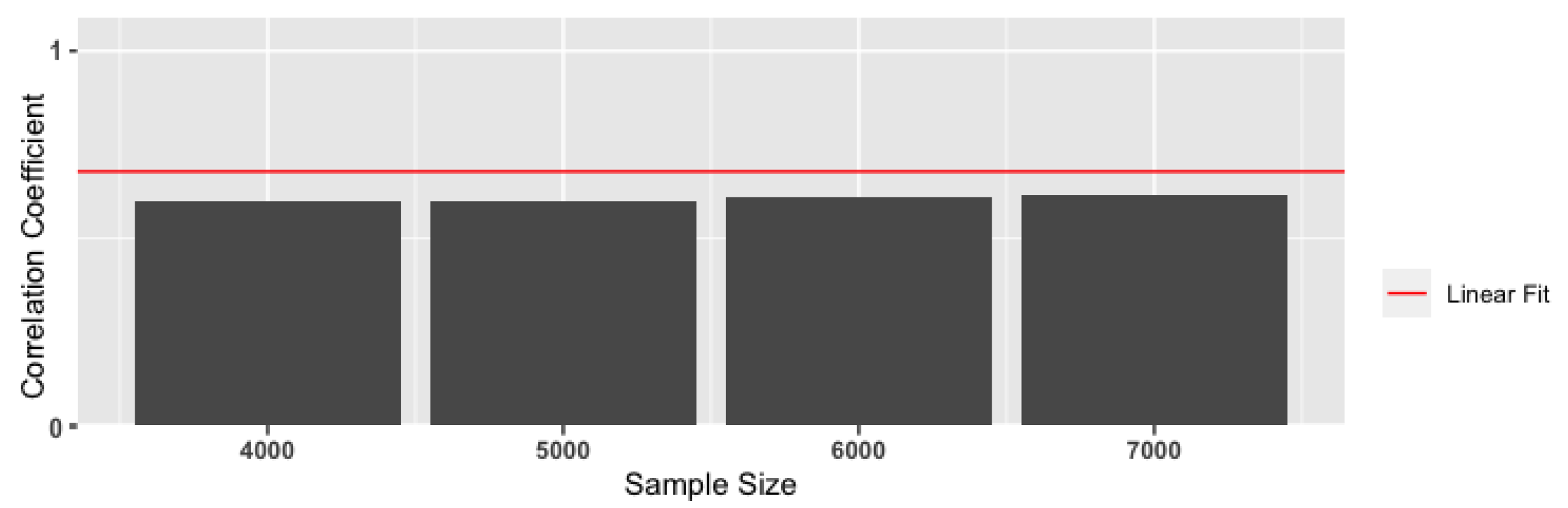
4.2.1. Similarity between True and Predicted Values
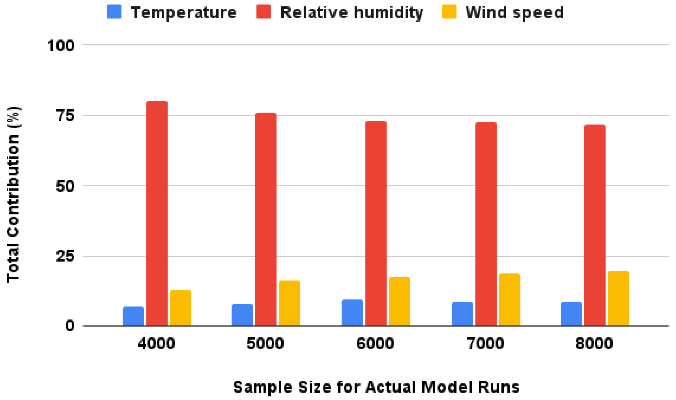
4.2.2. Scenario Analysis through Sensitivity Analysis to Input Parameters
4.2.3. Reduced Computational Requirements
5. Conclusions and Future Work
Author Contributions
Funding
Institutional Review Board Statement
Informed Consent Statement
Data Availability Statement
Acknowledgments
Conflicts of Interest
References
- Kaizer, J.S.; Heller, A.K.; Oberkampf, W.L. Scientific computer simulation review. Reliab. Eng. Syst. Saf. 2015, 138, 210–218. [Google Scholar] [CrossRef]
- KC, U.; Garg, S.; Hilton, J.; Aryal, J.; Forbes-Smith, N. Cloud Computing in natural hazard modeling systems: Current research trends and future directions. Int. J. Disaster Risk Reduct. 2019, 38, 101188. [Google Scholar] [CrossRef]
- Vasconcelos, M.; Guertin, D.; Zwolinski, M. FIREMAP: Simulation of Fire Behavior—A GIS Supported System; General Technical Report; United States Department of Agriculture Forest Service: Washington, DC, USA, 1990; pp. 217–221. [Google Scholar]
- Coleman, J.R.; Sullivan, A.L. A real-time computer application for the prediction of fire spread across the Australian landscape. Simulation 1996, 67, 230–240. [Google Scholar] [CrossRef]
- Plourde, F.; Doan-Kim, S.; Dumas, J.; Malet, J. A new model of wildland fire simulation. Fire Saf. J. 1997, 29, 283–299. [Google Scholar] [CrossRef]
- Finney, M.A. FARSITE, Fire Area Simulator–Model Development and Evaluation; Number 4; US Department of Agriculture, Forest Service, Rocky Mountain Research Station: Ogden, UT, USA, 1998. [Google Scholar]
- Perry, G.L.; Sparrow, A.D.; Owens, I.F. A GIS-supported model for the simulation of the spatial structure of wildland fire, Cass Basin, New Zealand. J. Appl. Ecol. 1999, 36, 502–518. [Google Scholar] [CrossRef]
- Eklund, P. A distributed spatial architecture for bush fire simulation. Int. J. Geogr. Inf. Sci. 2001, 15, 363–378. [Google Scholar] [CrossRef]
- Lopes, A.; Cruz, M.; Viegas, D. FIRESTATION–An integrated system for the simulation of wind flow and fire spread over complex topography. In Proceedings of the III International Conference on Forest Fire Research and 14th Conference on Fire and Forest Meteorology, Luso, Portugal, 16–20 November 1998; pp. 16–20. [Google Scholar]
- Committee, C.S. Prometheus User Manual, v. 3.0. 1; Canadian Forest Service. Available online: https://prometheus.io/docs/introduction/overview/ (accessed on 24 May 2021).
- Miller, C.; Hilton, J.; Sullivan, A.; Prakash, M. SPARK–A bushfire spread prediction tool. In Proceedings of the International Symposium on Environmental Software Systems, Melbourne, VIC, Australia, 25–27 March 2015; Springer: Berlin, Germany, 2015; pp. 262–271. [Google Scholar]
- Tolhurst, K.; Shields, B.; Chong, D. Phoenix: Development and application of a bushfire risk management tool. Aust. J. Emerg. Manag. 2008, 23, 47–54. [Google Scholar]
- Matthews, S.; Fox-Hughes, P.; Grootemaat, S.; Hollis, J.J.; Kenny, B.J.; Sauvage, S. Australian Fire Danger Rating System: Research Prototype; International Association of Wildland Fire: Missoula, MT, USA, 2019; p. 384. [Google Scholar]
- KC, U.; Garg, S.; Hilton, J. An efficient framework for ensemble of natural disaster simulations as a service. Geosci. Front. 2020, 11, 1859–1873. [Google Scholar] [CrossRef]
- Sobol’, I.M. On sensitivity estimation for nonlinear mathematical models. Mat. Model. 1990, 2, 112–118. [Google Scholar]
- Cukier, R.; Fortuin, C.; Shuler, K.E.; Petschek, A.; Schaibly, J. Study of the sensitivity of coupled reaction systems to uncertainties in rate coefficients. I Theory. J. Chem. Phys. 1973, 59, 3873–3878. [Google Scholar] [CrossRef]
- Saltelli, A.; Tarantola, S.; Chan, K.S. A quantitative model-independent method for global sensitivity analysis of model output. Technometrics 1999, 41, 39–56. [Google Scholar] [CrossRef]
- Krzykacz-Hausmann, B. Epistemic sensitivity analysis based on the concept of entropy. In Proceedings of the SAMO2001, Madrid, Spain, 18–20 June 2001; pp. 31–35. [Google Scholar]
- Plischke, E.; Borgonovo, E.; Smith, C.L. Global sensitivity measures from given data. Eur. J. Oper. Res. 2013, 226, 536–550. [Google Scholar] [CrossRef]
- Pianosi, F.; Wagener, T. A simple and efficient method for global sensitivity analysis based on cumulative distribution functions. Environ. Model. Softw. 2015, 67, 1–11. [Google Scholar] [CrossRef]
- Freissinet, C.; Vauclin, M.; Erlich, M. Comparison of first-order analysis and fuzzy set approach for the evaluation of imprecision in a pesticide groundwater pollution screening model. J. Contam. Hydrol. 1999, 37, 21–43. [Google Scholar] [CrossRef]
- Richardson, A.D.; Hollinger, D.Y. Statistical modeling of ecosystem respiration using eddy covariance data: Maximum likelihood parameter estimation, and Monte Carlo simulation of model and parameter uncertainty, applied to three simple models. Agric. For. Meteorol. 2005, 131, 191–208. [Google Scholar] [CrossRef]
- Bachmann, A.; Allgöwer, B. Uncertainty propagation in wildland fire behaviour modelling. Int. J. Geogr. Inf. Sci. 2002, 16, 115–127. [Google Scholar] [CrossRef]
- Hilton, J.E.; Stephenson, A.G.; Huston, C.; Swedosh, W. Polynomial Chaos for sensitivity analysis in wildfire modelling. In Proceedings of the International Congress on Modelling and Simulation, Hobart, Australia, 3–8 December 2017; pp. 3–8. [Google Scholar]
- Wagener, T.; Kollat, J. Numerical and visual evaluation of hydrological and environmental models using the Monte Carlo analysis toolbox. Environ. Model. Softw. 2007, 22, 1021–1033. [Google Scholar] [CrossRef]
- Ekstrom, P.A. Eikos: A Simulation Toolbox for Sensitivity Analysis in Matlab. FACILIA AB. 2005. Available online: https://baixardoc.com/preview/eikos-a-simulation-toolbox-for-sensitivity-analysis-5c9a8be15eec9 (accessed on 12 March 2021).
- D’Augustine, A.F. MATLODE: A MATLAB ODE Solver and Sensitivity Analysis Toolbox. Ph.D. Thesis, Virginia Tech, Blacksburg, VA, USA, 2018. [Google Scholar]
- Pianosi, F.; Sarrazin, F.; Wagener, T. A Matlab toolbox for global sensitivity analysis. Environ. Model. Softw. 2015, 70, 80–85. [Google Scholar] [CrossRef]
- Herman, J.; Usher, W. SALib: An open-source Python library for sensitivity analysis. J. Open Source Softw. 2017, 2, 97. [Google Scholar] [CrossRef]
- Dutfoy, A.; Dutka-Malen, I.; Pasanisi, A.; Lebrun, R.; Mangeant, F.; Gupta, J.S.; Pendola, M.; Yalamas, T. OpenTURNS, an Open Source initiative to Treat Uncertainties, Risks’ N Statistics in a structured industrial approach. In Proceedings of the 41èmes Journées de Statistique, SFdS, Bordeaux, France, 25–29 May 2009. [Google Scholar]
- Preisler, H.K.; Chen, S.C.; Fujioka, F.; Benoit, J.W.; Westerling, A.L. Wildland fire probabilities estimated from weather model-deduced monthly mean fire danger indices. Int. J. Wildland Fire 2008, 17, 305–316. [Google Scholar] [CrossRef]
- Pimont, F.; Fargeon, H.; Opitz, T.; Ruffault, J.; Barbero, R.; Martin-StPaul, N.; Rigolot, E.; Rivière, M.; Dupuy, J.L. Prediction of regional wildfire activity in the probabilistic Bayesian framework of Firelihood. Ecol. Appl. 2021, 31, e02316. [Google Scholar] [CrossRef] [PubMed]
- Ager, A.A.; Barros, A.M.; Day, M.A.; Preisler, H.K.; Spies, T.A.; Bolte, J. Analyzing fine-scale spatiotemporal drivers of wildfire in a forest landscape model. Ecol. Model. 2018, 384, 87–102. [Google Scholar] [CrossRef]
- Preisler, H.K.; Westerling, A.L.; Gebert, K.M.; Munoz-Arriola, F.; Holmes, T.P. Spatially explicit forecasts of large wildland fire probability and suppression costs for California. Int. J. Wildland Fire 2011, 20, 508–517. [Google Scholar] [CrossRef]
- Penman, T.D.; Cirulis, B.; Marcot, B.G. Bayesian decision network modeling for environmental risk management: A wildfire case study. J. Environ. Manag. 2020, 270, 110735. [Google Scholar] [CrossRef]
- Mendes, J.M.; de Zea Bermudez, P.C.; Pereira, J.; Turkman, K.; Vasconcelos, M. Spatial extremes of wildfire sizes: Bayesian hierarchical models for extremes. Environ. Ecol. Stat. 2010, 17, 1–28. [Google Scholar] [CrossRef]
- Joseph, M.B.; Rossi, M.W.; Mietkiewicz, N.P.; Mahood, A.L.; Cattau, M.E.; St. Denis, L.A.; Nagy, R.C.; Iglesias, V.; Abatzoglou, J.T.; Balch, J.K. Spatiotemporal prediction of wildfire size extremes with Bayesian finite sample maxima. Ecol. Appl. 2019, 29, e01898. [Google Scholar] [CrossRef]
- Cisneros, D.; Gong, Y.; Yadav, R.; Hazra, A.; Huser, R. A combined statistical and machine learning approach for spatial prediction of extreme wildfire frequencies and sizes. arXiv 2021, arXiv:2112.14920. [Google Scholar] [CrossRef]
- KC, U.; Hilton, J.; Garg, S.; Aryal, J. A probability-based risk metric for operational wildfire risk management. Environ. Model. Softw. 2022, 148, 105286. [Google Scholar] [CrossRef]
- KC, U.; Aryal, J. Leveraging a wildfire risk prediction metric with spatial clustering. Fire 2022, 5, 213. [Google Scholar] [CrossRef]
- KC, U.; Garg, S.; Hilton, J.; Aryal, J. An adaptive quadtree-based approach for efficient decision making in wildfire risk assessment. Environ. Model. Softw. 2022, 160, 105590. [Google Scholar] [CrossRef]
- Carriger, J.F.; Thompson, M.; Barron, M.G. Causal Bayesian networks in assessments of wildfire risks: Opportunities for ecological risk assessment and management. Integr. Environ. Assess. Manag. 2021, 17, 1168–1178. [Google Scholar] [CrossRef] [PubMed]
- Khakzad, N. Modeling wildfire spread in wildland-industrial interfaces using dynamic Bayesian network. Reliab. Eng. Syst. Saf. 2019, 189, 165–176. [Google Scholar] [CrossRef]
- Storey, M.A.; Bedward, M.; Price, O.F.; Bradstock, R.A.; Sharples, J.J. Derivation of a Bayesian fire spread model using large-scale wildfire observations. Environ. Model. Softw. 2021, 144, 105127. [Google Scholar] [CrossRef]
- Jaafari, A.; Gholami, D.M.; Zenner, E.K. A Bayesian modeling of wildfire probability in the Zagros Mountains, Iran. Ecol. Inform. 2017, 39, 32–44. [Google Scholar] [CrossRef]
- Silva, G.L.; Soares, P.; Marques, S.; Dias, M.I.; Oliveira, M.M.; Borges, J.G. A Bayesian modelling of wildfires in Portugal. In Dynamics, Games and Science; Springer: Berlin, Germany, 2015; pp. 723–733. [Google Scholar]
- Zwirglmaier, K.; Papakosta, P.; Straub, D. Learning a Bayesian network model for predicting wildfire behavior. In Proceedings of the ICOSSAR 2013, New York, NY, USA, 16–20 June 2013. [Google Scholar]
- KC, U.; Garg, S.; Hilton, J.; Aryal, J. A cloud-based framework for sensitivity analysis of natural hazard models. Environ. Model. Softw. 2020, 134, 104800. [Google Scholar] [CrossRef]
- KC, U.; Aryal, J.; Hilton, J.; Garg, S. A Surrogate Model for Rapidly Assessing the Size of a Wildfire over Time. Fire 2021, 4, 20. [Google Scholar] [CrossRef]
- Lindgren, F.; Rue, H. Bayesian spatial modelling with R-INLA. J. Stat. Softw. 2015, 63, 1–25. [Google Scholar] [CrossRef]
- Gelfand, A.E.; Smith, A.F. Sampling-based approaches to calculating marginal densities. J. Am. Stat. Assoc. 1990, 85, 398–409. [Google Scholar] [CrossRef]
- Simpson, D.; Rue, H.; Riebler, A.; Martins, T.G.; Sørbye, S.H. Penalising model component complexity: A principled, practical approach to constructing priors. Stat. Sci. 2017, 32, 1–28. [Google Scholar] [CrossRef]
- Chib, S. Marginal likelihood from the Gibbs output. J. Am. Stat. Assoc. 1995, 90, 1313–1321. [Google Scholar] [CrossRef]
- Spiegelhalter, D.J.; Best, N.G.; Carlin, B.P.; Van Der Linde, A. Bayesian measures of model complexity and fit. J. R. Stat. Soc. Ser. B (Stat. Methodol.) 2002, 64, 583–639. [Google Scholar] [CrossRef]
- Watanabe, S. A widely applicable Bayesian information criterion. J. Mach. Learn. Res. 2013, 14, 867–897. [Google Scholar]
- Pettit, L. The conditional predictive ordinate for the normal distribution. J. R. Stat. Soc. Ser. B (Methodol.) 1990, 52, 175–184. [Google Scholar] [CrossRef]
- Spark: Predicting Bushfire Spread. Available online: https://data61.csiro.au/en/Our-Research/Our-Work/Safety-and-Security/Disaster-Management/Spark (accessed on 12 May 2021).
- Tasmania. List Data. 2021. Available online: https://listdata.thelist.tas.gov.au/opendata/ (accessed on 12 March 2021).
- Tasmania Fire Service. State Fire Commission Annual Report; Tasmania Fire Service: Hobart, Australia, 2019. [Google Scholar]
- Ujjwal, K.C.; Garg, S.; Hilton, J.; Aryal, J. Fire Simulation Data Set for Tasmania; CSIRO: Canberra, Australia, 2021. [Google Scholar] [CrossRef]
- Saltelli, A. Making best use of model evaluations to compute sensitivity indices. Comput. Phys. Commun. 2002, 145, 280–297. [Google Scholar] [CrossRef]
- Benesty, J.; Chen, J.; Huang, Y.; Cohen, I. Pearson correlation coefficient. In Noise Reduction in Speech Processing; Springer: Berlin, Germany, 2009; pp. 1–4. [Google Scholar]


| Priors | Parameters Name | Parameters Value |
|---|---|---|
| half-Cauchy | mean, scale | (0, 25) |
| half-t | mean, shape | (0, 3) |
| log-gamma | shape, rate | (1, 0.00005) |
| half-normal | mean, precision | (0, 0.001) |
| PC log-gamma | shape, rate | (5, 0.01) |
| uniform improper | standard deviation () |
| Parameters | Unit | Range | |
|---|---|---|---|
| Temperature | C | Uniform Distribution | [10, 40] |
| Relative Humidity | % | Uniform Distribution | [5, 90] |
| Wind Speed | Uniform Distribution | [10, 60] |
| Components | With Latent Process | Without Latent Process |
|---|---|---|
| MLK | 64,329.60 | 64,561.05 |
| DIC | 128,586.56 | 128,945.93 |
| WAIC | 128,584.76 | 129,008.34 |
| 8.04 | 8.063 |
Disclaimer/Publisher’s Note: The statements, opinions and data contained in all publications are solely those of the individual author(s) and contributor(s) and not of MDPI and/or the editor(s). MDPI and/or the editor(s) disclaim responsibility for any injury to people or property resulting from any ideas, methods, instructions or products referred to in the content. |
© 2023 by the authors. Licensee MDPI, Basel, Switzerland. This article is an open access article distributed under the terms and conditions of the Creative Commons Attribution (CC BY) license (https://creativecommons.org/licenses/by/4.0/).
Share and Cite
KC, U.; Aryal, J.; Bakar, K.S.; Hilton, J.; Buyya, R. Applying Bayesian Models to Reduce Computational Requirements of Wildfire Sensitivity Analyses. Atmosphere 2023, 14, 559. https://doi.org/10.3390/atmos14030559
KC U, Aryal J, Bakar KS, Hilton J, Buyya R. Applying Bayesian Models to Reduce Computational Requirements of Wildfire Sensitivity Analyses. Atmosphere. 2023; 14(3):559. https://doi.org/10.3390/atmos14030559
Chicago/Turabian StyleKC, Ujjwal, Jagannath Aryal, K. Shuvo Bakar, James Hilton, and Rajkumar Buyya. 2023. "Applying Bayesian Models to Reduce Computational Requirements of Wildfire Sensitivity Analyses" Atmosphere 14, no. 3: 559. https://doi.org/10.3390/atmos14030559
APA StyleKC, U., Aryal, J., Bakar, K. S., Hilton, J., & Buyya, R. (2023). Applying Bayesian Models to Reduce Computational Requirements of Wildfire Sensitivity Analyses. Atmosphere, 14(3), 559. https://doi.org/10.3390/atmos14030559